A STATIC APPROACH TO THE N ELSON -S

M

ASTER OF

S

CIENCE IN

F

INANCE

M

ASTER

´

S

F

INAL

W

ORK

D

ISSERTATION

A

STATIC APPROACH TO THE

N

ELSON

-S

IEGEL

-S

VENSSON MODEL

:

APPLICATION TO

SEVERAL NEGATIVE YIELDS CASES

V

ÍTOR

H

UGO

F

ERREIRA

C

ARVALHO

ii

M

ASTER OF

S

CIENCE IN

F

INANCE

M

ASTER

´

S

F

INAL

W

ORK

D

ISSERTATION

A

STATIC APPROACH TO THE

N

ELSON

-S

IEGEL

-S

VENSSON MODEL

:

APPLICATION TO

SEVERAL NEGATIVE YIELDS CASES

V

ÍTOR

H

UGO

F

ERREIRA

C

ARVALHO

S

:

M

T

M

G

iii

A

The appearance of negative bond yields presents significant challenges to the fixed

income markets, mainly to the adjust and forecasting methods. The

Nelson-Siegel-Svensson model (NSS) is in most cases adopted by central banks to estimate the term

structure of interest rates.

In this study, it was chosen the NSS model to fit the yield curves of a set of countries

which registered negative sovereign bond yields. No changes or constraints were done

to the model or its parameters. It was applied with friendly, widely available, and simple

tools. The model adjusted well for all countries yield curves, even with partial bond

yields data. A comparison between market instantaneous interest rate and interest rate

for a very distant future, that the model can predict, was done, with good results for the

instantaneous interest rate.

Since the main set of countries, included in the study, are within the Eurozone, an

evaluation of a shared debt securities (i.e. Eurobonds) possible behaviour was analysed.

The NSS model can be a valuable, easy to use and adaptable tool, to fit the yield curve

with negative yields, for the use of the monetary policy institutions and market players,

at least in a static way.

JEL Classification: C02; C18; E43; E47; G12; G17

Key Words: yield curve; negative bond yields; Eurobonds; Nelson-Siegel-Svensson

iv

R

O aparecimento de obrigações com taxas de juro negativas apresenta desafios

significativos para os mercados de rendimento fixo, principalmente com os métodos de

ajuste e previsão. O modelo de Nelson-Siegel-Svensson (NSS) é, na maioria dos casos,

adotado pelos bancos centrais para estimar a estrutura a prazo das taxas de juros.

Neste estudo, foi escolhido o modelo NSS para ajustar as curvas de taxa de juro de um

conjunto de países que registaram obrigações soberanas com taxas de juro negativas.

Não foram feitas alterações ou restrições ao modelo ou aos seus parâmetros. Foi

aplicado com ferramentas amigáveis, amplamente disponíveis e simples. O modelo

ajustou-se bem para todas as curvas de taxa dos países, mesmo com dados parciais de

taxas de juro das obrigações. Uma comparação entre a taxa de juros instantânea do

mercado e a taxa de juro para um futuro muito distante, que o modelo pode prever, foi

feito, com bons resultados para a taxa de juro instantânea.

Uma vez que o principal conjunto de países, incluído no estudo, está dentro da zona do

Euro, foi analisado o possível comportamento de uma dívida partilhada (ou seja,

Eurobonds).

O modelo NSS pode ser uma ferramenta valiosa, fácil de usar e adaptável, para ajustar

a curva de taxas de juro negativas, para uso das instituições de política monetária e dos

operadores do mercado, pelo menos de forma estática.

Classificação JEL: C02; C18; E43; E47; G12; G17

Palavras-chave: curva de taxas de juro; taxas de juro negativas de obrigações;

v

A

I would like to thank my supervisor Professor Maria Teresa Medeiros Garcia for her

support, generous guidance and suggestions through the entire process for this Master

Final Work.

To my Mother, Father, Brother and Friends, I would like to give a special and profound

thank you, for their support, belief and enthusiasm.

To Tânia, for her love, for being my essence and the greatest Woman on Cosmos. You

are the only person that truly knows and understands who I am. I love to share my

journey on this point in space with You. Unforgettable, that´s what you are…

Inês and Amélia, you are the reason for everything. Your smiles and hugs are so pure

and sincere. My babies, you show me a wonderful life.

vi

I

Abstract ... iii

Resumo ... iv

Acknowledgments ... v

Tables Index ... vi

Figures Index ... vi

1 Introduction ... 1

2 Literature review... 4

3 Methodology ... 8

3.1 Data ... 12

3.2 Analysis... 15

4 Results and discussion... 22

5 Conclusions ... 25

6 References ... 27

Appendices ... 30

Appendix I – Countries data ... 30

Appendix II – Countries market and NSS model yield curves ... 33

Appendix III – Countries market and NSS model yield curves (short term forecast) ... 37

Appendix IV – Countries market and NSS model yield curves (intermediate term forecast) ... 41

Appendix V – Countries market and NSS model yield curves (long term forecast) ... 45

T

I

Table II - Countries data under ECB monetary policy ... 30

Table III - Countries data not under ECB monetary policy ... 30

Table IV - Countries data under ECB monetary policy (theoretical value considered as the YTM of the lowest maturity bond - 1 year) – IRVDF ... 31

Table V - Countries data not under ECB monetary policy (theoretical value considered as the YTM of the lowest maturity bond - 1 year) – IRVDF ... 31

Table VI - Countries data under ECB monetary policy (observed value considered as the YTM of the highest maturity bond - 1 year) – IRVDF ... 32

Table VII - Countries data not under ECB monetary policy (observed value considered as the YTM of the highest maturity bond - 1 year) – IRVDF ... 32

Table VIII - NSS model 1,2,3,4 and 1,2 factors (fitting the entire yield curve) ... 33

Table IX - NSS model 1,2,3,4 and 1,2 factors (short term maturities forecast) ... 37

Table X - NSS model 1,2,3,4 and 1,2 factors (intermediate term maturities forecast) ... 41

Table XI - NSS model 1,2,3,4 and 1,2 factors (long term maturities forecast) ... 45

F

I

Figure 2 - Convex and non-convex function ... 16

vii

Figure 4 - IRVDF ... 19

Figure 5 - IRVDF (with theoretical value considered as the YTM of the lowest maturity bond (1 year) .... 19

Figure 6 - IRVDF (with observed value considered as the YTM of the highest maturity bond ... 19

Figure 7 - European countries yield curves ... 20

Figure 8 - European countries yield curves (maturities until 10 years) ... 20

Figure 9 - Excess rate related to Germany... 21

Figure 10 - Austria market and NSS yield curve (March 15, 2017) ... 33

Figure 11 - Belgium market and NSS yield curve (May 5, 2017) ... 33

Figure 12 - Bulgaria market and NSS yield curve (May 5, 2017) ... 33

Figure 13 - Czech Republic market and NSS yield curve (May 5, 2017) ... 33

Figure 14 - Denmark market and NSS yield curve (March 15, 2017) ... 34

Figure 15 - Finland market and NSS yield curve (March 15, 2017) ... 34

Figure 16 - France market and NSS yield curve (March 15, 2017) ... 34

Figure 17 - Germany market and NSS yield curve (March 16, 2017) ... 34

Figure 18 - Ireland market and NSS yield curve (May 5, 2017) ... 34

Figure 19 - Italy market and NSS yield curve (May 5, 2017) ... 34

Figure 20 - Japan market and NSS yield curve (March 16, 2017) ... 35

Figure 21 - Lithuania market and NSS yield curve (May 5, 2017) ... 35

Figure 22 - Luxembourg market and NSS yield curve (May 5, 2017) ... 35

Figure 23 - Netherlands market and NSS yield curve (March 15, 2017) ... 35

Figure 24 - Portugal market and NSS yield curve (May 5, 2017) ... 35

Figure 25 - Slovakia market and NSS yield curve (May 5, 2017) ... 35

Figure 26 - Slovenia market and NSS yield curve (May 5, 2017) ... 36

Figure 27 - Spain market and NSS yield curve (May 5, 2017) ... 36

Figure 28 - Sweden market and NSS yield curve (March 15, 2017) ... 36

Figure 29 - Switzerland market and NSS yield curve (March 15, 2017) ... 36

Figure 30 - Austria market and NSS yield curve (March 15, 2017) - STF ... 37

Figure 31 - Belgium market and NSS yield curve (May 5, 2017) - STF ... 37

Figure 32 - Bulgaria market and NSS yield curve (May 5, 2017) - STF ... 37

Figure 33 - Czech Republic market and NSS yield curve (May 5, 2017) - STF ... 37

Figure 34 - Denmark market and NSS yield curve (March 15, 2017) - STF... 38

Figure 35 - Finland market and NSS yield curve (March 15, 2017) - STF ... 38

Figure 36 - France market and NSS yield curve (March 15, 2017) - STF ... 38

Figure 37 - Germany market and NSS yield curve (March 16, 2017) - STF ... 38

Figure 38 - Ireland market and NSS yield curve (May 5, 2017) - STF ... 38

Figure 39 - Italy market and NSS yield curve (May 5, 2017) - STF ... 38

Figure 40 - Japan market and NSS yield curve (March 16, 2017) - STF ... 39

Figure 41 - Lithuania market and NSS yield curve (May 5, 2017) - STF ... 39

Figure 42 - Luxembourg market and NSS yield curve (May 5, 2017) - STF... 39

Figure 43 - Netherlands market and NSS yield curve (March 15, 2017) - STF ... 39

Figure 44 - Portugal market and NSS yield curve (May 5, 2017) - STF ... 39

Figure 45 - Slovakia market and NSS yield curve (May 5, 2017) - STF ... 39

Figure 46 - Slovenia market and NSS yield curve (May 5, 2017) - STF ... 40

Figure 47 - Spain market and NSS yield curve (May 5, 2017) - STF... 40

Figure 48 - Sweden market and NSS yield curve (March 15, 2017) - STF ... 40

Figure 49 - Switzerland market and NSS yield curve (March 15, 2017) - STF ... 40

Figure 50 - Austria market and NSS yield curve (March 15, 2017) - ITF... 41

Figure 51 - Belgium market and NSS yield curve (May 5, 2017) - ITF ... 41

Figure 52 - Bulgaria market and NSS yield curve (May 5, 2017) - ITF ... 41

viii

Figure 54 - Denmark market and NSS yield curve (March 15, 2017) - ITF ... 42

Figure 55 - Finland market and NSS yield curve (March 15, 2017) - ITF ... 42

Figure 56 - France market and NSS yield curve (March 15, 2017) - ITF ... 42

Figure 57 - Germany market and NSS yield curve (March 16, 2017) - ITF ... 42

Figure 58 - Ireland market and NSS yield curve (May 5, 2017) - ITF ... 42

Figure 59 - Italy market and NSS yield curve (May 5, 2017) - ITF ... 42

Figure 60 - Japan market and NSS yield curve (March 16, 2017) - ITF ... 43

Figure 61 - Lithuania market and NSS yield curve (May 5, 2017) - ITF ... 43

Figure 62 - Luxembourg market and NSS yield curve (May 5, 2017) - ITF ... 43

Figure 63 - Netherlands market and NSS yield curve (March 15, 2017) - ITF ... 43

Figure 64 - Portugal market and NSS yield curve (May 5, 2017) - ITF ... 43

Figure 65 - Slovakia market and NSS yield curve (May 5, 2017) - ITF ... 43

Figure 66 - Slovenia market and NSS yield curve (May 5, 2017) - ITF ... 44

Figure 67 - Spain market and NSS yield curve (May 5, 2017) - ITF ... 44

Figure 68 - Sweden market and NSS yield curve (March 15, 2017) - ITF ... 44

Figure 69 - Switzerland market and NSS yield curve (March 15, 2017) - ITF ... 44

Figure 70 - Austria market and NSS yield curve (March 15, 2017) - LTF ... 45

Figure 71 - Belgium market and NSS yield curve (May 5, 2017) - LTF ... 45

Figure 72 - Bulgaria market and NSS yield curve (May 5, 2017) - LTF ... 45

Figure 73 - Czech Republic market and NSS yield curve (May 5, 2017) - LTF ... 45

Figure 74 - Denmark market and NSS yield curve (March 15, 2017) - LTF ... 46

Figure 75 - Finland market and NSS yield curve (March 15, 2017) - LTF ... 46

Figure 76 - France market and NSS yield curve (March 15, 2017) - LTF... 46

Figure 77 - Germany market and NSS yield curve (March 16, 2017) - LTF ... 46

Figure 78 - Ireland market and NSS yield curve (May 5, 2017) - LTF ... 46

Figure 79 - Italy market and NSS yield curve (May 5, 2017) - LTF ... 46

Figure 80 - Japan market and NSS yield curve (March 16, 2017) - LTF ... 47

Figure 81 - Lithuania market and NSS yield curve (May 5, 2017) - LTF ... 47

Figure 82 - Luxembourg market and NSS yield curve (May 5, 2017) - LTF ... 47

Figure 83 - Netherlands market and NSS yield curve (March 15, 2017) - LTF ... 47

Figure 84 - Portugal market and NSS yield curve (May 5, 2017) - LTF ... 47

Figure 85 - Slovakia market and NSS yield curve (May 5, 2017) - LTF ... 47

Figure 86 - Slovenia market and NSS yield curve (May 5, 2017) - LTF ... 48

Figure 87 - Spain market and NSS yield curve (May 5, 2017) - LTF ... 48

Figure 88 - Sweden market and NSS yield curve (March 15, 2017) - LTF ... 48

Figure 89 - Switzerland market and NSS yield curve (March 15, 2017) - LTF ... 48

1

1

I

The existence of negative bond yields presents significant challenges to the fixed income

markets. Some, are related to the modelling and forecasting methods, others are due to

the actual size of assets with negative yields ($13,4 trillion, Financial Times, 2016) and,

finally, one can detect the impact on financial theory and the implications for bond

holders and issuers.

As the Nelson and Siegel model (1987) and proposed extension of Svensson (1994) are

in most cases adopted by central banks to estimate the term structure of interest rates

(BIS, 2005), the Nelson-Siegel-Svensson (NSS) model was chosen in this study to fit the

yield curves of a set of countries which registered negative, sovereign bond yields.

Negative yields are recent and can in some way be an outcome of some important

aspects. The 2008 financial crisis lead Federal Reserve (Fed) to start quantitative easing

programs1 _{until October 29}th_{, 2014, later followed by European Central Bank (ECB) (ECB,}

2017a) in the aftermath of 2010/2011 European government debt crisis and the

significant reduction in the directorate interest rate of ECB. Japan with its lost decades2

(Hayashi & Prescott, 2002) and low rates, combined presently, with China and world

GDP reduction growth, had lead the fixed income markets to search for “safe heavens”.

These “safe heavens” issuers are the ones that have higher ratings and, so can provide

higher certainty that will service entirely their debts. In a certain way, the high debt

1 _{Available at:}

https://www.thebalance.com/what-is-quantitative-easing-definition-and-explanation-3305881 | https://www.ecb.europa.eu/explainers/show-me/html/app_infographic.en.html Accessed date: August 7th_{, 2017}

2 _{Hayashi and Prescott, used the expression “Lost decade” to refer to Japan 1990s economic stagnation,}

2

levels of European Union countries, and the highest debt of the world, like in Japan

(234% of the GDP in 2015) (OECD, 2017), should demand greater yields for these issuers,

but ratings (that seem to be more favourable to developed countries (Cantor & Packer,

1996)) and the lack of possibility for the emerging countries to capture the fixed income

markets with intensity, have conduct to the present situation characterized by higher

debts issuers related to their GDP with, in some cases, the lowest yields, and, awkwardly,

cases of negative yields, that are something not so predictable and common.

Given that the market players (e.g. insurance companies, pension funds, banks) have

the need to estimate and model the term structure of interest rates with these recent

negative bond yields, this work contributes to solve this matter, proposing the use of

NSS model, by means of friendly, widely available, and simple tools. Hence, the

objectives of this study are:

• to evaluate the adequacy of the NSS model through the fit of the yield curve, at a

certain date, with at least one negative yield value and, through the interest rates

values that one can deduct from the model, compared with market data, with a

easy to use approach; and,

• to evaluate the results of the model with partial market bond yields data (short,

intermediate and long-term).

Thus, the present work is composed, in addition to Introduction, by the literature

review, the methodology, the results and the conclusion chapters, regarding the two

main objectives above mentioned.

The literature review chapter intends to present and describe the model chosen, it´s

application and importance, as well as the approaches done to fit negative yields market

3

In the methodology chapter, the NSS model and parameters are described in detail, as

well as the calibration method, the analysis procedure, the data and software definitions

to accomplish data analysis.

The results chapter collects the main outcomes of the work and leads the way to new

studies. Indeed, given that the greater set of countries are European and in the

Eurozone, it will be taken the opportunity to see a comparison between their yield

curves and some effects of a possible future shared Eurozone debt security (i.e.

4

2

L

The term structure of interest rates, or yield curve, is a key variable of economics and

finance (Büttler, 2007). The direct relation between term structure of interest rates and

yield curve, should be clarified. Málek (2005), in Hladíková & Radová (2012), places the

distinction to three equivalent descriptions of the term structure of interest rates:

• the discount function, which specifies zero-coupon bond prices as a function of

maturity;

• the spot yield curve, which specifies zero-coupon bond yields (spot rates) as a

function of maturity;

• the forward yield curve, which specifies zero-coupon bond forward yields (forward

rates) as a function of maturity.

The discount function, entails some undesirable conditions. Bond prices are insensitive

to yields changes for shorter maturities, and minimizing price errors, sometimes, results

in large yield errors for bonds for those shorter maturities (Svensson, 1994). Also,

monetary policy makers and economic discussions, generally, focus on interest rates

rather than prices (Geyer & Mader, 1999). For these reasons, the discount function,

could not be a suitable description of the term structure of interest rates.

To the purpose of an entire evaluation of the yield curve (maturities can be as high as

30, 50 and even 100 years), the forward market products are not adequate since they

have a short time limit, so the forward yield curve can be a proper description of the

yield curve for the shorter maturities.

In case of the spot yield curve, the market has no zero-coupon bonds for all maturities,

5

should be considered. The use of coupon bond, with different coupon rates, instead of

zero-coupon bonds, have negligible impact, in accordance to Kariya et al (2013, in Inui,

2015). Svensson (1994) mentioned that to get implied forward interest rates from yield

to maturity (YTM) on coupon bonds is more complicated than on zero coupon bonds.

The YTM obtained from market data will give, implied spot rates, instead of real spot

rates, since one cannot compute, the entire yield curve with all maturities (i.e. spot yield

curve), from zero-coupon bond yields. Although, Cox et al (1985) stated that “the

expectations hypothesis postulates that bonds are priced so that the implied forward

rates are equal to the expected spot rates”.Synthesising, the term structure of interest

rates or yield curve, is computed through YTM of government coupon bonds, and

through that, one will get the implied rates.

One of the objectives and usefulness to fit the yield curve is to provide the monetary

policy institutions with indicators of rates evolution and expectations (e.g. inflation). The

need for the monetary policy institutions to have these indicators, increased when

flexible exchange rates have replaced fixed exchange rates (Svensson, 1994). Other

significant purpose is related to fixed income market participants (e.g. hedging

strategies, assets allocation for pension funds).

To fit the yield curve there are several methods. Based on Sundaresan (2009)

compilation, these include:

• the Vasicek (1977) model is a mean reversion process. Allows negative rates, but

doesn´t calibrate with market data;

• the Rendleman and Bartter (1980) model follows a simple multiplicative random

walk. Rates are assumed to be lognormally distributed, which invalidates its use in

6

• the Cox, Ingersoll and Ross (CIR) model (Cox et al, 1985) it´s a mean reversion

model, but doesn´t allow negative interest rates and doesn´t calibrate with

market data;

• the Ho and Lee (1986) model, is calibrated to market yields. Assumes a normal

distribution of interest rates and interest rates can become negative;

• the Black, Derman and Toy (1990) (BDT) model can be calibrated through market

equity options data, but assumes that rates follow a lognormally distribution,

which invalidates its use in the case of negative yields. Combines mean reversion

and volatility;

• the Black and Karasinski (1991) model is calibrated to market yields and volatilities.

Separates mean reversion and volatility;

• the Nelson and Siegel (1987) and Svensson (1994) extension is an exponential

function to approximate the unknown forward rate function;

• the Bootstrapping method will generate a zero-coupon yield curve from existing

market data such as bond prices, but lacks robustness (Martellini et al, 2003).

It was beyond our purpose to use all models. It was used the NSS since the purpose of

this study is to get a model calibrated with market data and to evaluate the interest

rates, from the model, without evaluate volatilities for yields or bond prices, as is

required on some other models. In fact, several curve fitting spline methods have been

criticized for having undesirable economic properties and for being ‘black box’ models

(Seber & Wild, 2003 in Annaert et al, 2010).

The NSS model is parsimonious and has been widely used in academia and in practice,

but is sensitive to the starting values of the parameters (1,2,3,4 and 1,2) (Annaert et al,

7

The NSS model respects the restrictions imposed by the economic and financial theory

(rates take real numbers and not complex ones and are higher for long-terms than for

shorter ones) and can take any yield curve form empirically observed in the market

(Diebold & Rudebusch, 2013, in Ibáñez, 2015). Moreover, if the NSS could work in a

negative yield market, this would be of most importance to hedging strategies (mainly

for market participants, to hedge against flattening or steepening of the yield curve) and

get forecasts for interest rates levels (very useful for monetary policy makers).

Another purpose is to fit the yield curve and get a static value of instantaneous interest

rate (IIR) and interest rate of a very distant future (IRVDF), and check if the values given

by the model are in accordance with the market ones. Additionally, one objective is to

use a friendly, widely available tool for a not so in-depth user of math tools or software.

It´s not a purpose to evaluate time evolution of the interest rates, based on the NSS

8

3

M

The yield curve (term structure of interest rates), that can be estimated from bond yields

of a certain economic region, is of utmost importance to monetary and economic

authorities to support decisions processes and stablish policies, as well as to market

participants for their investments and actions (Martellini et al, 2003).

In this work, it was chosen a curve fitting statistical model (like NSS model) to check if it

works with negative yields and all along the yield curve. In some cases, oscillating in

signal (i.e. positive and/or negative) yield values. The NSS model is a curve fitting model

that can provide us with values for instantaneous and distant future interest rates.

The approach taken does not add more factors, parameters nor terms to the current

NSS model. It computes all yield curves for each of the selected countries and tries to

get economic and financial data to evaluate the forecast adequacy of the model, even

in cases of issuers with few negative yields. Hence, it is not an objective of this work to

study the NSS model parameters time series nor forecast its values to get a yield curve

evolution. It was adopted a static fitting to check how NSS model works with negative

yields at some part of the yield curve.

The Nelson Siegel model and Svensson extension, Equation (1), is a parametric

curve-fitting method procedure, is statistical in their approach, and generally do not have a

sound economic foundation.

(1)

Svensson (1994) extension adds a new factor, with a new decay parameter, Equation

(2), to improve a better fit. As clearly described by Guedes (2008), for the Nelson Siegel

model, there can be an economic interpretation of the parameters.

𝜸(𝜽) = 𝜷𝟏+ 𝜷𝟐[𝟏 − 𝒆 − 𝜽_𝝀

𝟏

𝜽 𝝀𝟏

] + 𝜷𝟑[ 𝟏 − 𝒆 − 𝜽_𝝀

𝟏

𝜽 𝝀𝟏

− 𝒆− 𝜽𝝀𝟏] + 𝜷_𝟒[𝟏 − 𝐞

− 𝜽_𝝀

𝟐

𝜽 𝝀𝟐

9

(2)

In this work, and since Svensson extension is an added component to the Nelson Siegel

model, to better fit the yield curve, it was considered to interpret the parameters as

they are defined for Nelson Siegel model:

• () is the yield to maturity value (spot rate) at the time of data collection with

maturity ;

• β1 is the IRVDF;

• β1+β2 is the initial value of the curve and can be interpreted as the IIR;

• -β2 is the spread between the interest rates of long and short times (i.e. average

slope of the curve);

• β1,2 and β3 determine how short and long interest rates interchange and are

responsible for the hump (inclination) that the yield curve shows.

• β4 is the extension of the model proposed by Svensson in 1994, that can be

interpreted as an independent decay parameter, that will introduce a new hump

to better fit the model;

•  is the maturity of the bond;

• 1 and 2 are parameters responsible for how inclination and curvature behave,

don´t have an economic interpretation although determine the interchange

between short and long interest rates.

Until negative bond yields appearance in some markets, NSS model did not present

much difficulties on its application and was widely used.

Guedes (2008) stated that 1+2>0, which for the paradigm of that time and until then

appeared to be a very reasonable economic and financial condition. The general

𝜷𝟒[𝟏 − 𝐞 − 𝜽_𝝀

𝟐

𝜽 𝝀𝟐

10

perception that rates, at least nominal ones (real rates, that consider other effects as

inflation, can be lower than zero) would always be positive, lead to the definition of

limits that the models should work. Central banks, like ECB for deposit facility rate, have

presently, nominal negative rates. Although, more frequent, cases of negative yields and

negative interest rates is even somehow something strange and awkward.

Time and markets have showed that 1+2 (interpreted as the IIR) can be lower than

zero. This study tries to show that there is an economical and real-world interpretation

for 1+2<0.

At a first approach, it is expected that the yield curve fitting, with some negative bond

yields, would be more difficult, due to the calibration process, which usually calculates

the minimum value of the sum of squared residuals (SSR). As stated by Svensson (1994),

the parameters are then chosen, so, as to minimize the sum of squared yield errors

between estimated and observed yields. The analysis done used the NSS model and SSR

without any kind of changes in the formulas. Gilli et al (2010) stated that one possibility

for the calibration is to use Equation (3) to calculate the SSR, being y the NSS model

calculated yield and yM _{the market yield value.}

(3) 𝑚𝑖𝑛

𝛽,𝜆 ∑(𝑦 − 𝑦 𝑀₎2

In this study, the market values were the bond yields for each maturity, for each country.

Then the NSS model would, through Microsoft Excel Solver (Frontline System, 2017a)

function, compute the residuals minimum value, and so, getting the values for the

parameters (1,2,3,4 and 1,2). The parametrization of Solver for the data used in this thesis,

11

For the forecasting purposes, only a few market bond yields maturities where given to

test and the NSS model ran to check if it could adjust the curve for the missing

maturities. Partial market data was considered following the classification of the

beginning of 1990´s, that bond markets used to bond maturities: short, intermediate

and long term (Martellini et al, 2003), being the most usual time frame for each division

as follow: bonds with maturities until 5 years are called short term bonds, from 5 to

10/12 years they are called intermediate bonds and higher than 10/12 years are called

long bonds.

When forecasting the NSS model for short term maturity bonds, the 5 years’ time frame,

couldn´t be considered as a fixed period, because the model didn´t produced good fitting

date. The NSS model seems to need at least one negative yield market data to proceed

with proper calibration and so provide parameters that could provide a reasonable

fitting curve. Taking this into consideration the short-term time frame was different for

every country and ranged from 2 to 5 years.

The intermediate period had its inferior limit defined by the higher value found from

short term forecast (STF). The upper limit was defined by the best observed fitting

depending on the mix of; always as possible to no more than 10 years (Lithuania is a

special case because has no bond maturities higher than 7 years), and the wider period

that could be considered with no market data to calibrate the model (Switzerland is a

special case where the limit is 25 years). This way it was defined the widest period, with

no market data, and that the NSS model produced parameters that result in a very good

12

The adequacy of NSS model to get parameter values (1,2,3,4 and 1,2) accurate enough,

with partial market data was evaluated for 3 sectors of the yield curve: short,

intermediate and long term.

For STF, the model calibrated, only, with market yields for intermediate and long-term

maturities, thus getting different values for the parameters as the ones obtained when

all the market data was used to calibrate the model. The parameters values and

countries yields curves with the lower forecast can be assessed in appendix II. Similarly,

the same was done when calculating the intermediate and long-term maturities

forecasts. For each of the forecast maturities, the model had access to only the other

maturities, for which computed the factors values that best fitted the curve. The Solver

function ran as much times as possible to get the best forecast fit values.

3.1

D

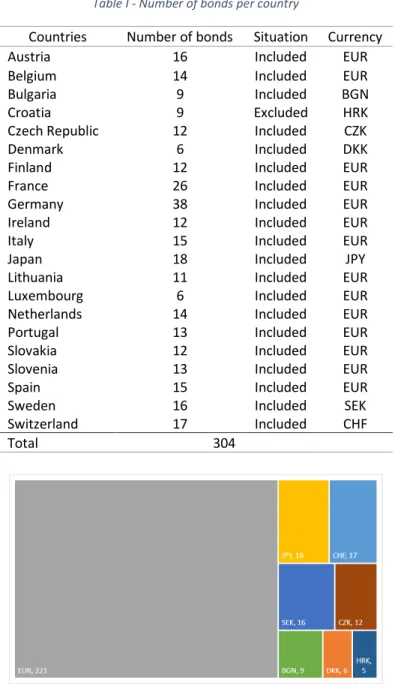
The study considers 304 different government bonds, from a group of 20 countries

(Austria, Belgium, Bulgaria, Czech Republic, Denmark, Finland, France, Germany,

Ireland, Italy, Japan, Lithuania, Luxembourg, Netherlands, Portugal, Slovakia, Slovenia,

Spain, Sweden and Switzerland) with at least one negative yield to maturity government

bond, at the date of data collection, March 15th_{, 2017 for the following issuer countries:}

Austria, Denmark, Finland, France, Netherlands, Sweden and Switzerland, March 16th_,

2017, for the following issuer countries: Germany, Japan, and May 5th_{, 2017 for the}

following issuer countries: Belgium, Bulgaria, Czech Republic, Ireland, Italy, Lithuania,

13

used to get bonds information used in the study, through a Bloomberg Terminal.

Inflation indexed bonds were not considered.

After a first approach to evaluate NSS model for the entire yield curve of countries

whose data was gathered at March 15th _{and 16}th _{2017, the set of issuers were extended}

to incorporate the other 11 countries that presented negative yield to maturity at May

5th_{, 2017. The extent of study countries was made taking into consideration two main}

purposes: first, to try to get more issuers to evaluate model adequacy to a wider set of

data; second, and because from the second set of countries they are mainly from Europe

and under ECB monetary policy, to try to get a wider, detailed and if possible, some

conclusion that could apply to Europe and/or Eurozone area.

From the actual 19 countries that compose Eurozone (European Union, 2017) (use the

Euro as their official currency and are under ECB monetary policy), 14 of them are

included in this study. The other 5 Eurozone countries (Cyprus, Estonia, Greece, Latvia

and Malta) were not included in the study, since they did not have any fixed income

security with a negative yield, at the study period; March 15th _{and 16}th_{, 2017 and May}

5th_{, 2017.}

Presently, European Union has 28 members (European Union, 2017), so, half of the

members had, at study dates, negative bond yields. Croatia had negative yields for the

period of 2016 end to beginning of 2017, although by the time of data collection (May

5th_{, 2017) yields for all maturities were positive.}

Table I and Figure 1 show how many different securities were used for each country as

well as the denomination currencies.

Tables II and III show the countries target of the study, their date of data collection,

14

Union, the β1 and β1+β2 theoretical values (obtained from the fitting process) it´s

observed values, and notes.

Table I - Number of bonds per country

Countries Number of bonds Situation Currency Austria 16 Included EUR Belgium 14 Included EUR Bulgaria 9 Included BGN

Croatia 9 Excluded HRK

Czech Republic 12 Included CZK

Denmark 6 Included DKK

Finland 12 Included EUR

France 26 Included EUR

Germany 38 Included EUR Ireland 12 Included EUR

Italy 15 Included EUR

Japan 18 Included JPY

Lithuania 11 Included EUR Luxembourg 6 Included EUR Netherlands 14 Included EUR Portugal 13 Included EUR Slovakia 12 Included EUR Slovenia 13 Included EUR

Spain 15 Included EUR

Sweden 16 Included SEK

Switzerland 17 Included CHF

Total 304

Figure 1 – Number of bonds per currency

Table II collects all countries under ECB monetary policy, so use Euro as their currency.

These countries share and are in the same currency risk and in the same rates referential

so they compose an important subset of the data sample. Table III collects all the other

cases. It wasn´t consider the European Union countries do to the fact that Bulgaria,

15

ECB and can control their currency exchange rate (Bulgaria has a fixed exchange rate to

the Euro). Tables IV and V are, respectively, to countries under ECB and the ones outside

ECB monetary policy. These tables show the data if it is considered the theoretical value,

for the IRVDF, the yield to maturity of the lowest maturity bond (1 year). Tables VI and

VII are, respectively, to countries under ECB and the ones outside ECB monetary policy.

These tables show the data considering the observed value, for the IRVDF, the yield to

maturity of the highest maturity bond.

3.2

A

The application of Solver function, to all bonds of the countries described in Data

chapter, took into consideration the following conditions: a GRG Non-linear algorithm

for the resolution method3_{, restriction precision value of 10}-8 _{(the standard value used}

by Solver is 10-6_{, a lower value will provide a more precise value, although increases the}

time Solver spends to get to a solution), it was used the default selection for Solver to

Use automatic rounding, the value chosen for the Convergence (value between 0 and 1)

was 10-8_{, it defines the upper limit for the relative change in destiny cell, for the last 5}

iterations, to define when Solver should stop (i.e. if in the last 5 iterations the relative

change in the value of the destination cell in less than 10-6_{%, then Solver stops to try to}

converge even more) (Microsoft, 2017a).

Since the results obtained with direct differentiation (default on Solver) were very good

considering that there wasn´t observed difference from the ones obtained for central

differentiation (for a few countries tested), also there were no message from Solver

16

mentioning it couldn´t improve, and because direct differentiation is much faster, it was

used direct differentiation for all yield curves fitting computation.

Solver uses a Generalized Reduced Gradient Algorithm for optimizing nonlinear

problems (Microsoft, 2017b), which, provides a locally optimal solution to a reasonably

well-scaled, non-convex model (Frontline System, 2017b). A function f is convex if the

function f is bellow any line segment between two points on f. Figure 2 is an adaptation

from Tomioka (2012) and shows an example of convex and non-convex function.

Figure 2 - Convex and non-convex function

The starting values for (1,2,3,4 and 1,2) should be in or as near as possible of the order of

magnitude of the expected values. Values near or below 0.01 for i and 1 to j were

used. After first solution provided by Solver, the parameters values were submitted to

small changes and the Solver function ran again, to get a SSR as low as possible. Only

when Solver provided the message that after 5 iterations the fitting curve hasn’t

changed, that solution was considered as the final one. It wasn´t applied any restrictions

to the values that (1,2,3,4 and 1,2) could take.

When modelling the entire yield curve, having NSS model access to all market yields

collects from the countries, to use in SSR, or when modelling the entire yield curve, with

part of the market data available (i.e. the cases of short-term, intermediate and

long-term, bonds maturities), the parameters (1,2,3,4 and 1,2) could take any value, and no

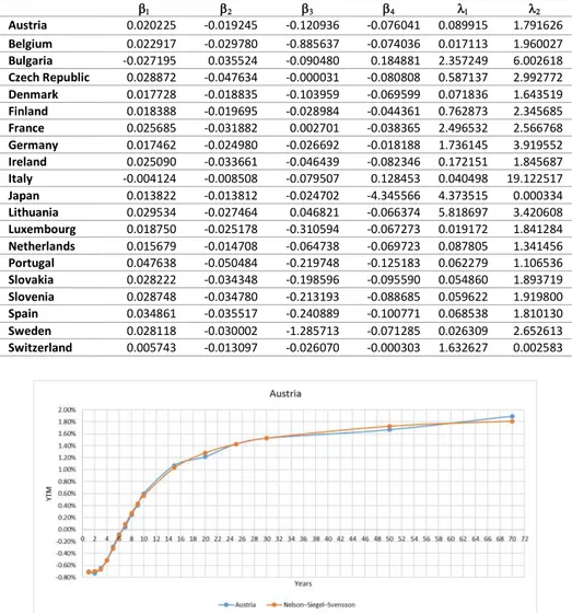
17

be accessed on Table VIII (NSS model used all market yields available), Table IX (short

term maturities forecast or simply STF), Table X (intermediate term maturities forecast

or simply, intermediate term forecast (ITF)) and Table XI (long term maturities forecast

or simply, long term forecast (LTF)).

It has been referred that β1 can be interpreted as the IRVDF and β1+β2 as the IIR. It was

considered in this study, the IIR, as the overnight rate (in practice, instantaneous rate

can be identified with an overnight forward rate (Svensson, 1994)) supervised by the

countries monetary policy institution. For countries under ECB rules the rate considered

is the unsecured overnight lending rate, Eonia®4 _{(Euro OverNight Index Average). Eonia®}

is the observed value that compares with the theoretical obtained from the NSS model.

The definition of a very distant future and its correspondent interest rate for that time

horizon is, in a certain way, a not concrete date. Due to market present situation of ECB

monetary easing policy that are intended to run until the end of December 2017, or

beyond, if necessary (ECB, 2017b), and considering the most time distant rate at which

Euro interbank term deposits are offered Euribor®5 _{12 months, this was the rate chosen}

as the observed value to compare with β1.

In Table III, due to the uniqueness of each country monetary policy institution the rates

considered to be the benchmark for β1 (IRVDF) and β1+β2 (IIR) are diversified. For the

β1+β2 it was chosen the corresponding overnight rate or then the repo rate with the

shorter time horizon (a repo rate is the rate at which banks can borrow from their

Central bank). Hladíková & Radová (2012) also used the repo rate to compare with the

4 _{Available at: https://www.emmi-benchmarks.eu/euribor-eonia-org/eonia-rates.html Accessed date:}

August 6th_{, 2017}

5 _{Available at: https://www.emmi-benchmarks.eu/euribor-org/about-euribor.html Accessed date:}

18

starting value of estimated forward rate. These two rates are very close to one another

(Martellini et al, 2003). Similarly, for β1 (IRVDF), it was chosen the corresponding rate

equivalent to the country´s Euribor.

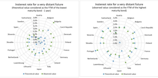
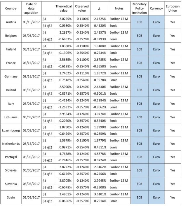
Theoretical and observed IRVDF and IIR can be compared on Figures 3 and 4 and Tables

II and III. As mentioned before, the definition of very distant future is not concrete, so it

was considered the following two changes when evaluating the data and analysis;

• theoretical value, considered as the YTM of the lowest maturity bond (1 year).

Data can be assessed on Tables IV and V, and Figure 5.

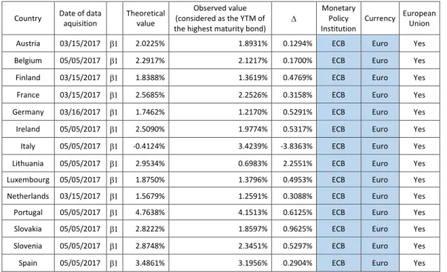
• observed value, considered as the YTM of the highest maturity bond. Data can be

assessed on Tables VI and VII, and Figure 6.

A descriptive statistical analysis (with the calculation of: mean, median, standard

deviation, kurtosis, asymmetry, minimum and maximum) was done to the differences

of the theoretical and observed values. This, alongside with comparison with theoretical

and observed values, can help to get more substantiated conclusions. This analysis was

applied to two sets of countries data (all study countries and then to the subset of

countries supervised by ECB) for both the IIR and the IRVDF.

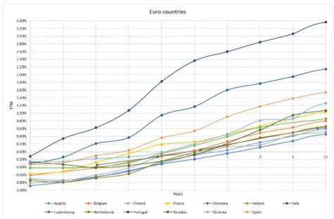
Since the main set of countries in the study are from Europe, it was compared all yield

curves (Figure 7) for these issuers. The spectrum of maturities that each country

chooses, or can access to, in the market, is very different, as well as the yields that each

one has, are very wide. The differences for the yield curves are related to the premiums

required by the market and are dependent on: ratings, political risk, GDP growth, debt

19

The 10-year maturity bonds yield is one of the most used and compared in financial

markets. For the set of European countries, only Lithuania hadn´t maturities higher than

7 years, so it cannot be compared with its fellow European countries.

Figure 3 - Theoretical and observed IIR Figure 4 – IRVDF (with observed value considered as Euribor 12 M)

Figure 5 - IRVDF (with theoretical value considered as the YTM of the lowest maturity bond (1 year))

Figure 6 - IRVDF (with observed value considered as the YTM of the highest maturity bond)

As a theoretical exercise, if European countries on the Eurozone agreed eventually on a

shared debt security (i.e. Eurobonds), it could, on an initial phase, be issued bonds with

20

choice. On Figure 8, one can see this set of countries (without Lithuania) and their yield

curves.

Figure 7 - European countries yield curves

Figure 8 - European countries yield curves (maturities until 10 years)

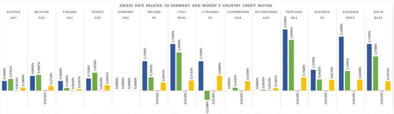
It was evaluated, for the Eurozone countries, if the differences seen, for the theoretical

and observed rates values, for β1 (IRVDF), could be explained by the excess rate, that

21

Sovereign CDS, net of US is 0.00%)6_{. It´s mentioned also the Moody´s credit ratings, for}

each country.

Figure 9, shows the differences, for the theoretical and observed rates values, for β1

(IRVDF), for two interpretations of the very distant future. One, the comparison between

Sovereign CDS, net of US (or net of Germany, since both have the same value) (blue bar)

and the Observed value, for β1, considered as the YTM of the highest maturity bond

(green bar). So, in case of Portugal, the excess rate that Portugal has related to Germany

is 2.9342%, this means that the YTM of its highest maturity bond is 2.9342% higher than

the YTM of the highest maturity bond of Germany, and the relation with the Sovereign

CDS, net of US is of the same sign and similar value.

The second set of comparisons that can be accessed on Figure 9, are between: observed

value for the β1 parameter (considered as Euribor 12 Months) and its difference with

Germany observed value (also, Euribor 12 Months) (red bar); and the difference

between, the theoretical value for β1 (considered as YTM of the lowest maturity bonds,

1 year) for each country and Germany (yellow bar).

Figure 9 - Excess rate related to Germany

6 _{Available at: http://pages.stern.nyu.edu/~adamodar/New_Home_Page/datafile/ctryprem.html}

22

4

R

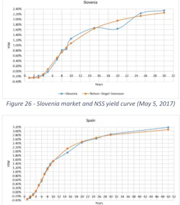
The NSS model fitting process, with no restrictions on the parameters values, adjusts

well the yield curve for the wide variety of countries and maturities range (appendix II).

It was pointed out that Nelson-Siegel model was not appropriate to be applied to Japan

Government Bonds market because it might show negative interest rate and abnormal

shape in short term region (Kikuchi & Shintani, 2012, in Inui, 2015). In this work, and

using NSS model, the curve shows a good fitting (Figure 20) and the difference between

the short interest rate, chosen as the observed value, and the theoretical one, is 0.044%,

which is a low value (Table III).

The values obtained for β1 and β1+β2, interpreted, as IRVDF (Figure 4 and Tables II and

III) and IIR respectively (Figure 3 and Tables II and III), show that theoretical and

observed values are closer to each other for the IIR, than for the IRVDF, who presents a

wider difference.

If the YTM of the highest maturity is considered the observed value for the IRVDF, the

values are very close to the theoretical ones. Specifically, the excess rate related to

Germany, can be almost fully explained.

The difference between theoretical and observed IIR, for the all sets of countries, has an

almost normal distribution (kurtosis=3.14) with: mean of -0.055%, median of 0.019%,

standard deviation of 0.644%, minimum of -1.926%, and a maximum of 1.233%. These

results show a very wide range, probably influenced by different monetary policies. The

same values, for the countries under ECB monetary policy, show a platykurtic

23

deviation of 0.429%, minimum of -0.906% and a maximum of 0.564%, which represents

a shorter range, suggesting the same monetary policy.

The difference between theoretical and observed IRVDF, for the all set of countries, has

a leptokurtic distribution (kurtosis=5.92), with: mean of 2.058%, median of 2.274%,

standard deviation of 1.688%, minimum of -3.501% and a maximum of 4.888%, showing

significant dispersion. The same values for the countries under ECB monetary policy,

show a platykurtic distribution (kurtosis=2.69), with: mean of 2.470%, median of

2.524%, standard deviation of 1.154%, minimum of -0.288% and a maximum of 4.888%,

which also shows a wide range.

NSS model theoretical values for β1 (IRVDF) are generally the value of the yield of the

longest maturity in the yield curve (except for the extreme cases of Bulgaria, Italy,

Lithuania and Sweden). In a certain way, this is the most very distant future that is

available for each country, so, if the highest maturity for each country is the market

interpretation of very distant future, then the model provides good values. Otherwise if

for “very distant future” one considers the one-year time frame, then the model is not

a proper one.

The results for short, intermediate and long-term forecasts, can be assessed,

respectively in appendices II, III and IV. The short-term forecast shows the model

difficulties to fit the yield curve, given that the beginning of the yield curves is less

smooth than the intermediate and long terms. Also, it is in the shorter term that

negative yields appear.

The intermediate and long-term forecasts show very acceptable fittings, in some cases

24

Considering the subset of countries and yield curves that can be seen on Figure 8, and if

eventually a shared debt security (i.e. Eurobonds) issue was done, the market would,

theoretically, lower the risk premium and the yields for the most stressed countries (the

ones that show higher yields). For the lower risk premium issuers, it will increase the

yields. Since, all countries would share the risk, these risk premiums reflected on yields,

could be a price to pay to get a more equal and more distressful financial system in the

Eurozone.

The evaluation of rate differences related to excess rate to Germany show that there is

a clear relation, Figure 9, between excess rate observed and the Sovereign CDS, net of

US, at least for the main set of countries considered. Only for Ireland, Lithuania and

Slovenia, the differences are higher than 1%. If it´s taken into consideration that bonds

data was gathered at least 3 months after the Sovereign CDS considered. The excess rate

25

5

C

The NSS model was applied to 20 countries and it shows that fits well the entire yield

curves, even for negative yields. It is a very friendly methodology and can be used with

a simple and widely available tool.

The forecast of the IIR can be improved, although the differences between theoretical

and observed values, appear to be small.

If, the IRVDF is considered the rate at the highest bond maturity, then the model,

presents good values.

The interpretation of the parameters for the NSS model as they are interpreted to

Nelson Siegel (NS) model, seems to be adequate.

In the case of countries under ECB monetary policy, the rate is defined by ECB, but, in

practice, European countries in the Eurozone are very different in essence (e.g.

economic models, debt levels, financial history, weight and importance on financial

markets). So, expecting them all to have the same rates, from the model, seems not be

a realistic hypothesis. It can be concluded that rates shouldn´t be all the same, since the

market is requesting a country risk premium (CPR) for each one, related to their ratings,

debt level, GDP, national budgets and deficits, political risk, among other factors. If

European countries under the Eurozone had the same debt securities, like Eurobonds,

then rates would be the same and yield curve would be only one, so the expected rates

values given by the NSS model could be more precise and a good proxy for the market

participants. Despite these results, Eurozone same debt securities could be target for

26

The excess rate related to Germany, by the Moody´s ratings and corresponding

Sovereign CDS, net of US (or Germany, since both countries share the same value) for

countries under ECB monetary policy, can be explained from the model parameters,

when considering the IRVDF to be the yield to maturity of highest maturity for that

country. The countries that presented a difference higher than 1%, are Ireland, Lithuania

and Slovenia.

The forecast outputs show good fitting data to real values for both intermediate term

and long-term maturities. On the other hand, short term forecasted values aren´t as

accurate as expected which leads to conclude that, in this case, it isn´t a good model.

The reasons for this can be the instability of monetary policy and the volatility of short

term interest rates.

Hence, the NSS model can be a valuable, easy to use and adaptable tool, to fit the yield

curve with negative yields, for the use of the monetary policy institutions and market

27

6

R

Annaert, J., Claes, A., Ceuster, M., Zhang, H. (2010). Estimating the Yield Curve Using the

Nelson-Siegel Model – A Ridge Regression Approach, Universiteit Antwerpen.

BIS (2005). Zero-coupon yield curves: technical documentation, BIS Papers, 25, Bank for

International Settlements.

Büttler, H. (2007). An Orthogonal Polynomial Approach to Estimate the Term Structure

of Interest Rates, Swiss National Bank Working Papers, 8.

Cantor, R. & Packer, F. (1996). Determinants and Impact of Sovereign Credit Ratings,

Federal Reserve Bank of New York, 37-53.

Cox, J. C., Ingersoll, J. E., Ross, S. A. (1985). A Theory of the Term Structure of Interest

Rates, Econometrica, 53 (2), 385-407.

ECB (2017a). Asset purchase programmes. Available at:

https://www.ecb.europa.eu/mopo/implement/omt/html/index.en.html

[Accessed date: August 7th_{, 2017].}

ECB (2017b). Monetary policy decisions. Press Release, 20 July 2017. Available at:

https://www.ecb.europa.eu/press/pr/date/2017/html/ecb.mp170720.en.html

[Accessed date: August 6th_{, 2017].}

European Union (2017). EU monetary cooperation. Available at:

https://europa.eu/european-union/about-eu/money/euro_en [Accessed date:

March 15th_{, 2017].}

Financial Times (2016). Value of negative-yielding bonds hits $13.4tn. Available at:

28

Frontline Systems (2017a). Excel Solver Online Help. Available at:

https://www.solver.com/excel-solver-online-help [Accessed date: August 8th_,

2017].

Frontline Systems (2017b). Excel Solver – GRG Nonlinear Solving Method Stopping

Conditions. Available at:

https://www.solver.com/excel-solver-grg-nonlinear-solving-method-stopping-conditions [Accessed date: June 15th_{, 2017].}

Geyer, A. & Mader, R. (1999). Estimation of the Term Structure of Interest Rates – A

Parametric Approach, Oesterreichische Nationalbank Working Paper 37.

Gilli, M., Große, S. and Schumann, E. (2010). Calibrating the Nelson-Siegel-Svensson

model, COMISEF Working Paper Series 31.

Guedes, J. (2008). Modelos Dinâmicos da Estrutura de Prazo das Taxas de Juro, IGCP

Instituto de Gestão da Tesouraria e do Crédito Público, I. P..

Hayashi, F. & Prescott, E. C. (2002). The 1990s in Japan: A Lost Decade, Review of

Economic Dynamics, 5 (1), 206-235.

Hladíková, H. & Radová, J. (2012). Term Structure Modelling by Using Nelson-Siegel

Model, European Financial and Accounting Journal, 7 (2), 36-55.

Ibáñez, F. (2015). Calibrating the Dynamic Nelson-Siegel Model: A Practitioner Approach,

Central Bank of Chile.

Inui, K. (2015). Improving Nelson-Siegel term structure model under zero / super-low

interest rate policy, Meiji University.

Martellini, L., Priaulet, P. and Priaulet, S. (2003). Fixed-Income Securities Valuation, Risk

Management and Portfolio Strategies, Wiley.

Microsoft (2017a). Função SolverOptions. Available at:

29

Microsoft (2017b). Solver Uses Generalized Reduced Gradient Algorithm. Available at:

https://support.microsoft.com/en-us/help/82890/solver-uses-generalized-reduced-gradient-algorithm [Accessed date: July 2nd_{, 2017].}

Nelson, C. & Siegel, A. (1987). Parsimonious Modelling of Yield Curve, Journal of

Business, 60, 473-489.

OECD (2017). General government debt (indicator). doi: 10.1787/a0528cc2-en; Available

at: https://data.oecd.org/gga/general-government-debt.htm [Accessed date:

June 17th_{, 2017].}

Sundaresan, S. (2009). Fixed Income Markets and Their Derivatives, Academic Press,

Third Edition.

Svensson, L. E. (1994). Estimating and Interpreting Forward Interest Rates: Sweden

1992-1994, Centre for Economic Policy Research Discussion Paper 1051.

Tomioka, R. (2012). Convex Optimization: Old Tricks for New Problems, The University of

30

A

A

I

–

C

Table II - Countries data under ECB monetary policy

Country Date of data aquisition Theoretical value Observed

value  Notes

Monetary Policy Institution

Currency European Union

Austria 03/15/2017  2.0225% -0.1100% 2.1325% Euribor 12 M ECB Euro Yes

 0.0980% -0.3540% 0.4520% Eonia

Belgium 05/05/2017  2.2917% -0.1240% 2.4157% Euribor 12 M ECB Euro Yes

 -0.6863% -0.3570% -0.3293% Eonia

Finland 03/15/2017  1.8388% -0.1100% 1.9488% Euribor 12 M ECB Euro Yes

 -0.1306% -0.3540% 0.2234% Eonia

France 03/15/2017  2.5685% -0.1100% 2.6785% Euribor 12 M ECB Euro Yes

 -0.6198% -0.3540% -0.2658% Eonia

Germany 03/16/2017  1.7462% -0.1110% 1.8572% Euribor 12 M ECB Euro Yes

 -0.7518% -0.3540% -0.3978% Eonia

Ireland 05/05/2017  2.5090% -0.1240% 2.6330% Euribor 12 M ECB Euro Yes

 -0.8571% -0.3570% -0.5001% Eonia

Italy 05/05/2017  -0.4124% -0.1240% -0.2884% Euribor 12 M ECB Euro Yes

 -1.2632% -0.3570% -0.9062% Eonia

Lithuania 05/05/2017  2.9534% -0.1240% 3.0774% Euribor 12 M ECB Euro Yes

 0.2070% -0.3570% 0.5640% Eonia

Luxembourg 05/05/2017  1.8750% -0.1240% 1.9990% Euribor 12 M ECB Euro Yes

 -0.6429% -0.3570% -0.2859% Eonia

Netherlands 03/15/2017  1.5679% -0.1100% 1.6779% Euribor 12 M ECB Euro Yes

 0.0971% -0.3540% 0.4511% Eonia

Portugal 05/05/2017  4.7638% -0.1240% 4.8878% Euribor 12 M ECB Euro Yes

 -0.2846% -0.3570% 0.0724% Eonia

Slovakia 05/05/2017  2.8222% -0.1240% 2.9462% Euribor 12 M ECB Euro Yes

 -0.6126% -0.3570% -0.2556% Eonia

Slovenia 05/05/2017  2.8705% -0.1240% 2.9945% Euribor 12 M ECB Euro Yes

 -0.6078% -0.3570% -0.2508% Eonia

Spain 05/05/2017  3.4861% -0.1240% 3.6101% Euribor 12 M ECB Euro Yes

 -0.0656% -0.3570% 0.2914% Eonia

Table III - Countries data not under ECB monetary policy

Country Date of data aquisition Theoretical value Observed

value  Notes

Monetary Policy Institution

Currency European Union

Bulgaria 05/05/2017

 -2.7195% 0.782% -3.5015% SOFIBOR (Sofia Interbank Offered Rate) Bulgarian National Bank

BGN Yes

31

Average) Reference Rate

Czech

Republic 05/05/2017

 2.8872% 0.0500% 2.8372% Deposit Facility Czech National

Bank

CZK Yes

 -1.8763% 0.0500%

-1.9263% 2W repo rate

Denmark 03/15/2017

 1.7728% 0.0950% 1.6778% CIBOR 12M Denmark National Bank

DNK Yes

 -0.1107% -0.4857% 0.3750% Tomorrow/next (T/N) Rate

Japan 03/16/2017

 1.3822% 0.3000% 1.0822%

Basic Discount Rates and Basic Loan Rates

Bank of

Japan Yen No

 0.0010% -0.0430% 0.0440%

Average value of Uncollateralized Overnight Call Rate for Mar. 16

Sweden 03/15/2017 

2.8118% -0.3650% 3.1768% STIBOR Fixing 6M Sweden National Bank

SEK Yes

 -0.1883% -0.5000% 0.3117% Repo rate

Switzerland 03/15/2017

 0.5743% -0.7300% 1.3043% 3-month LIBOR

CHF Swiss National

Bank

CHF No

 -0.7354% -0.7300% -0.0054%

SARON (formerly repo overnight index (SNB))

Table IV - Countries data under ECB monetary policy (theoretical value considered as the YTM of the lowest maturity bond - 1 year) – IRVDF

Country

Date of data aquisition

Theoretical value (considered as the YTM

of the lowest maturity bond, 1 year)

Observed

value  Notes

Monetary Policy Institution

Currency European Union

Austria 03/15/2017 -0.7037% -0.1100% -0.5937% Euribor 12M ECB Euro Yes

Belgium 05/05/2017 -0.6123% -0.1240% -0.4883% Euribor 12M ECB Euro Yes

Finland 03/15/2017 -0.8094% -0.1100% -0.6994% Euribor 12M ECB Euro Yes

France 03/15/2017 -0.5786% -0.1100% -0.4686% Euribor 12M ECB Euro Yes

Germany 03/16/2017 -0.8841% -0.1110% -0.7731% Euribor 12M ECB Euro Yes

Ireland 05/05/2017 -0.4194% -0.1240% -0.2954% Euribor 12M ECB Euro Yes

Italy 05/05/2017 -0.3088% -0.1240% -0.1848% Euribor 12M ECB Euro Yes

Lithuania 05/05/2017 -0.0152% -0.1240% 0.1088% Euribor 12M ECB Euro Yes

Luxembourg 05/05/2017 -0.3402% -0.1240% -0.2162% Euribor 12M ECB Euro Yes Netherlands 03/15/2017 -0.7479% -0.1100% -0.6379% Euribor 12M ECB Euro Yes Portugal 05/05/2017 -0.1181% -0.1240% 0.0059% Euribor 12M ECB Euro Yes Slovakia 05/05/2017 -0.2671% -0.1240% -0.1431% Euribor 12M ECB Euro Yes

Slovenia 05/05/2017 -0.2533% -0.1240% -0.1293% Euribor 12M ECB Euro Yes

Spain 05/05/2017 -0.3368% -0.1240% -0.2128% Euribor 12M ECB Euro Yes

Table V - Countries data not under ECB monetary policy (theoretical value considered as the YTM of the lowest maturity bond - 1 year) – IRVDF

Country

Date of data aquisition

Theoretical value (considered as the YTM of the lowest maturity bond - 1

year)

Observed

value  Notes

Monetary Policy Institution

Currency European Union

Bulgaria 05/05/2017 0.0960% 0.7820% -0.6860%

SOFIBOR (Sofia Interbank

Bulgarian

32

Offered Rate) Czech

Republic 05/05/2017 -0.4917% 0.0500% -0.5417% Deposit Facility

Czech

National Bank CZK Yes

Denmark 03/15/2017 -0.6339% 0.0950% -0.7289% CIBOR 12M

Denmark

National Bank DNK Yes

Japan 03/16/2017 -0.2303% 0.3000% -0.5303% Basic Discount and Basic Loan Rates

Bank of Japan Yen No

Sweden 03/15/2017 -0.5647% -0.3650% -0.1997% STIBOR Fixing 6M

Sweden

National Bank SEK Yes

Switzerland 03/15/2017 -0.9485% -0.7300% -0.2185%

3-month LIBOR CHF

Swiss National

Bank CHF No

Table VI - Countries data under ECB monetary policy (observed value considered as the YTM of the highest maturity bond - 1 year) – IRVDF

Country Date of data aquisition

Theoretical value

Observed value (considered as the YTM of the highest maturity bond)



Monetary Policy Institution

Currency European Union

Austria 03/15/2017  2.0225% 1.8931% 0.1294% ECB Euro Yes

Belgium 05/05/2017  2.2917% 2.1217% 0.1700% ECB Euro Yes

Finland 03/15/2017  1.8388% 1.3619% 0.4769% ECB Euro Yes

France 03/15/2017  2.5685% 2.2526% 0.3158% ECB Euro Yes

Germany 03/16/2017  1.7462% 1.2170% 0.5291% ECB Euro Yes

Ireland 05/05/2017  2.5090% 1.9774% 0.5317% ECB Euro Yes

Italy 05/05/2017  -0.4124% 3.4239% -3.8363% ECB Euro Yes

Lithuania 05/05/2017  2.9534% 0.6983% 2.2551% ECB Euro Yes Luxembourg 05/05/2017  1.8750% 1.3796% 0.4953% ECB Euro Yes Netherlands 03/15/2017  1.5679% 1.2591% 0.3088% ECB Euro Yes Portugal 05/05/2017  4.7638% 4.1513% 0.6125% ECB Euro Yes

Slovakia 05/05/2017  2.8222% 1.8597% 0.9625% ECB Euro Yes

Slovenia 05/05/2017  2.8748% 2.3451% 0.5297% ECB Euro Yes

Spain 05/05/2017  3.4861% 3.1956% 0.2904% ECB Euro Yes

Table VII - Countries data not under ECB monetary policy (observed value considered as the YTM of the highest maturity bond - 1 year) – IRVDF

Country Date of data aquisition Theoretical value Observed value (considered as the YTM of the highest maturity bond)

 Monetary Policy _Institution Currency European Union

Bulgaria 05/05/2017  -2.7195% 1.6040% -4.3235% Bulgarian National

Bank BGN Yes Czech

Republic 05/05/2017  2.8872% 2.3068% 0.5804% Czech National Bank CZK Yes Denmark 03/15/2017  1.7728% 1.1336% 0.6391% Denmark National Bank DNK Yes

Japan 03/16/2017  1.3822% 0.9289% 0.4533% Bank of Japan Yen No

Sweden 03/15/2017  2.8118% 1.7023% 1.1095% Sweden National Bank SEK Yes