www.atmos-chem-phys.net/10/9/2010/
© Author(s) 2010. This work is distributed under the Creative Commons Attribution 3.0 License.
Chemistry
and Physics
A comprehensive evaluation of seasonal simulations of ozone in the
northeastern US during summers of 2001–2005
H. Mao1, M. Chen2, J. D. Hegarty1, R. W. Talbot1, J. P. Koermer3, A. M. Thompson4, and M. A. Avery5 1Institute for the Study of Earth, Oceans, and Space, Climate Change Research Center, University of New Hampshire, Durham, 03824, New Hampshire, USA
2The Earth and Sun Systems Laboratory, National Center of Atmospheric Research, Boulder, 80305, Colorado, USA 3Department of Atmospheric Science & Chemistry, Plymouth State University, Plymouth, 03264, New Hampshire, USA 4Department of Meteorology, Pennsylvania State University, University Park, 16802, Pennsylvania, USA
5NASA Langley Research Center, Chemistry and Dynamics Branch, Hampton, 23681, Virginia, USA Received: 23 July 2009 – Published in Atmos. Chem. Phys. Discuss.: 1 September 2009
Revised: 2 December 2009 – Accepted: 9 December 2009 – Published: 5 January 2010
Abstract. Regional air quality simulations were conducted for summers 2001–2005 in the eastern US and subjected to extensive evaluation using various ground and airborne measurements. A brief climate evaluation focused on trans-port by comparing modeled dominant map types with ones from reanalysis. Reasonable agreement was found for their frequency of occurrence and distinctness of circulation pat-terns. The two most frequent map types from reanalysis were the Bermuda High (22%) and passage of a Canadian cold frontal over the northeastern US (20%). The model captured their frequency of occurrence at 25% and 18% respectively. The simulated five average distributions of 1-h ozone (O3) daily maxima using the Community Multiscale Air Quality (CMAQ) modeling system reproduced salient features in ob-servations. This suggests that the ability of the regional cli-mate model to depict transport processes accurately is crit-ical for reasonable simulations of surface O3. Comparison of mean bias, root mean square error, and index of agree-ment for CMAQ summer surface 8-h O3daily maxima and observations showed−0.6±14 nmol/mol, 14 nmol/mol, and 71% respectively. CMAQ performed best in moderately pol-luted conditions and less satisfactorily in highly polpol-luted ones. This highlights the common problem of overestimat-ing/underestimating lower/higher modeled O3levels. Diag-nostic analysis suggested that significant overestimation of inland nighttime low O3mixing ratios may be attributed to underestimates of nitric oxide (NO) emissions at night. The absence of the second daily peak in simulations for the Ap-pledore Island marine site possibly resulted from coarse grid resolution misrepresentation of land surface type.
Compari-Correspondence to:H. Mao ([email protected])
son with shipboard measurements suggested that CMAQ has an inherent problem of underpredicting O3 levels in con-tinental outflow. Modeled O3 vertical profiles exhibited a lack of structure indicating that key processes missing from CMAQ, such as lightning produced NO and stratospheric in-trusions, are important for accurate upper tropospheric rep-resentations.
1 Introduction
Air quality in New England is especially susceptible to vari-ations in seasonal climate due to its extensive areal forest coverage, complex terrain features, and significant influx of air pollutants from major urban/industrial centers in the east-ern US. There is already strong evidence that the length of the growing season is increasing in New England (New Eng-land Regional Assessment Group, 2001). Longer and hotter summers can have a major impact on air quality and the oc-currence of O3episodes via chemical and physical processes. To provide an assessment of the current environment, it is imperative to evaluate model performance for simulations of present day air quality.
diurnal variation underestimated. Van Loon et al. (2007) conducted an intercomparison of one-year simulations from seven regional air quality models and suggested that mixing ratios at night and in winter were more difficult to reproduce than during day- and summer due to difficulties of represent-ing a stable atmosphere accurately in models. In their three summer simulations, Vivanco et al. (2009) found fair agree-ment between model and measureagree-ments at rural sites in Spain with the exception of significant underestimation of O3 lev-els over the surrounding Madrid metropolis possibly due to poor representation of precursor transport in the model. Most model-observation comparison studies were conducted on a domain and multi-season average basis. However, besides providing such overall comparison, this study examined our modeling systems particularly in their performance of cap-turing episodes embedded in multiple seasons using exten-sive observations from field campaigns. We believe that our model evaluation here is thus more rigorous than previous studies and can provide insight on possible causes for model-observation discrepancies through evaluation of case studies. A quite common problem in model simulated O3 levels has been underestimation of high O3 values, which conse-quently makes it difficult to predict O3exceedance days re-liably, with one exception that Huang et al. (2007) showed realistically simulated summer ozone peaks, especially for the northeastern US averaged over the summer season and the subdomain. Zhang et al. (2006a, b) attributed underpre-diction in daily maximum 1-h O3mixing ratios on high O3 days to overpredicted planetary boundary layer (PBL) height. On most low O3 days uncertainties in O3 precursor emis-sions and overestimated surface layer vertical mixing led to inaccurate results. Yu et al. (2008) revealed that during their four-day simulation the underprediction of peak O3 concen-trations on high-O3days was caused by underrepresentation of regional contributions and local production to a lesser ex-tent. Results from these studies allude to the critical impor-tance of accurate simulations of processes depicting dynam-ics and physdynam-ics in the planetary boundary layer (PBL) to re-produce observed O3distributions.
A few studies included comparison of modeled upper level O3mixing ratios with measurements. Ozonesonde data have recently been used to evaluate models (Mao et al., 2006; Chai et al., 2007; Pierce et al., 2007; Tarasick et al., 2007; Yu et al., 2007). Mena-Carrasco et al. (2007) compared simulated O3using their regional air quality model STEM with NASA DC-8 and NOAA WP-3 airborne measurements during Inter-national Consortium for Atmospheric Research on Transport and Transformation (ICARTT) 2004 and found a strong posi-tive surface level bias and a negaposi-tive upper tropospheric bias. The low altitude and mid-tropospheric bias was reduced by using improved emission inventories, whereas the upper tro-pospheric bias was predominately affected by boundary con-ditions that were the output of global models.
In this study, we conducted an evaluation of multi-season regional climate and air quality model simulations for
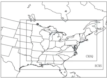
CMAQ
RCMS
Fig. 1.The RCMS and CMAQ domains.
summers (1 June–30 September) 2001–2005 over the east-ern US. We evaluated the performance of the climate and air quality models with a focus on transport processes and O3mixing ratios. A unique aspect of this study was that in addition to evaluating models on the domain and seasonal average basis, we examined their ability to represent pollu-tion episodes embedded in the five summer ensemble. To do that, we utilized measurements from a suite of observing platforms encompassing long-term ground-based networks, the NOAA ship Ronald H. Brown, aircraft, ozonesondes, radiosondes, the field campaigns New England Air Quality Study (NEAQS) 2002 and ICARTT 2004 intensive studies, and our 2004 Duke Forest, North Carolina (NC) intensive studies.
2 Models, data, and methods
2.1 Climate model
Pollard et al. (1995). RCMS was run over the time period of 1 May–30 September for each year of 2001–2005.
2.2 Emission model
The EPA emission model Sparse Matrix Operator Kernel Emissions (SMOKE) Modeling System was used to produce gridded emission data over the five summers. The most recent version of EPA emission model SMOKE with MO-BILE6 and BEIS3 was used with the 1999 NEI data. It was interfaced with the RCMS output to generate gridded emis-sion data for the seasonal air quality simulations.
2.3 Photochemical model
The Community Multi-scale Air Quality model (CMAQ) (Byun and Schere, 2006) was employed to simulate the dis-tributions of pollutants with the first three days as spin-up days over 1 June–30 September of 2001–2005. The 36 km horizontal grid structure in CMAQ follows that of MM5 with 72×59 cells which is marked as CMAQ in Fig. 1. Vertically there were 21 layers with the first 13 layers (from the sur-face up) identical to those in RCMS to maintain high reso-lution in the PBL. The CB-IV chemistry mechanism (Gery et al., 1989) was used due to its applicability and wide us-age in regional-scale modeling and its lesser computational demand compared to other schemes, which is particularly important for multi-seasonal runs. The cloud and aerosol modules were both used in this study. The cloud module included parameterizations for sub-grid convective precipi-tating and non-precipiprecipi-tating clouds and grid-scale resolved clouds. Cloud effects were included for both gas-phase species and aerosols. The aerosol module used an approach that represents the particle size distribution as the superpo-sition of three lognormal subdistributions, namely modes. The module calculates the concentrations of both PM2.5and PM10and includes estimates of the primary emissions of ele-mental and organic carbon, dust and other species not further specified. Secondary aerosol species considered were sul-fate, nitrate, ammonium, water, and organics from precursors of anthropogenic and biogenic origins.
2.4 Map typing
The modeled transport processes were evaluated by compar-ing the dominant circulation patterns from reanalysis data and model runs which were classified using the map typing technique (Lund, 1963). The NCEP Global Final Analysis (FNL) products are available for four time intervals each day (00:00, 06:00, 12:00, and 18:00 UTC) on a 1◦×1◦ global horizontal grid (http://dss.ucar.edu/datasets/ds083.2). For the evaluation of the circulation patterns we extracted the rean-alyzed and modeled sea level pressure fields at 12:00 UTC from FNL and RCMS respectively. The synoptic-scale cir-culation patterns were classified by applying the correlation-based map typing algorithm of Lund (1963) to the RCMS
and NCEP FNL sea level pressure (SLP) fields. This tech-nique has been successfully applied to synoptic classifica-tion of summertime circulaclassifica-tion patterns over the northeast-ern United States (Hegarty et al., 2009, 2007; Hogrefe et al., 2004). The algorithm calculates a correlation coefficient be-tween the grids representing scalar meteorological analysis fields over a given spatial domain at different times. The map types were selected using a critical correlation coeffi-cient (i.e., 0.65), and then all days in a given study period were classified as one of these types based on the degree of correlation. A minimum group size equal to 5% of the to-tal number of maps in each set (NCEP FNL or RCMS) was utilized to eliminate map types with few members.
2.5 Field measurements
Model output was evaluated using observed meteoro-logical and chemical data from: (1) National Weather Service radiosondes (http://vortex.plymouth.edu/get raob-u. html), (2) TDL US and Canada Surface Hourly Ob-servations (http://dss.ucar.edu/datasets/ds472.0; Vincentet al., 2007), (3) UNH AIRMAP air quality monitor-ing network (http://www.airmap.unh.edu), (4) surface ob-servations onboard the NOAA ship Ronald H. Brown
in NEAQS 2002 (http://www.esrl.noaa.gov/csd/NEAQS/ RonBrown) and ICARTT 2004 (http://www.esrl.noaa.gov/ csd/ICARTT/fieldoperations/fomp.shtml), (5) Environmen-tal Protection Agency AIRNOW sites in the northeast-ern US (http://airnow.gov/), (6) ozone soundings from the IONS Ozonesonde Network Study during ICARTT 2004 (http://croc.gsfc.nasa.gov/intex/ions.html) (Mao et al., 2006; Thompson et al., 2007a), and (7) the 4-week intensive at Duke Forest (Mao et al., 2008).
3 General characteristics of simulated seasonal climate
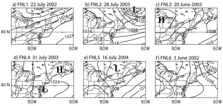
Fig. 2.The representative sea level pressure (SLP) in hPa distribution for map types FNL1- FNL6 and the date of occurrence.
processes. In our study, wind speed was better simulated at night than in daytime, and was in general under-predicted by the model by 3 m s−1. Modeled wind direction lagged obser-vations by 4.5◦C on average.
Simulations above the surface layer were evaluated using twice daily (00:00 and 12:00 UTC) vertical sounding data be-low 2 km from the twenty sites within the RCMS domain as illustrated in Fig. 1. The model underpredicted temperature by<2◦C in all levels and specific humidity by≤1 g kg−1. Wind speed was overpredicted by≤1 m s−1 except in lay-ers 2–4 where the average was≤2 m s−1, while wind direc-tion was simulated fairly accurately.
Transport processes are important in redistributing air-borne pollutants and thus model simulations of these pro-cesses need to be evaluated. One way to do that is to com-pare the modeled and observed dominant circulation patterns for the summers of 2001–2005. Note that we used the FNL from the NCEP to extract circulation patterns approximat-ing the real world. The map typapproximat-ing analysis identified six map types from the NCEP FNL analyses (denoted as FNL1-FNL6, Fig. 2) and five map types from the RCMS simula-tions (denoted as RCM1-RCM5, Fig. 3). A total of 70% of the days could be classified as one of the FNL types and 77% of the days could be classified as one of the RCMS types. The frequency of occurrence of each map type and the corresponding meteorological conditions are summarized in Table 1.
The FNL1 map type (Fig. 2a) representing the Bermuda High circulation was the most common of the NCEP FNL types (22%) and featured light south-southwest flow over much of the northeastern US Similarly, RCM1 (Fig. 3a)
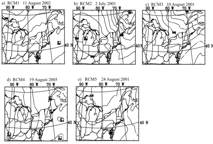
occurred on 25% of the days with great resemblance to FNL1, and its higher frequency of occurrence suggests a slight tendency for RCMS to over-predict the occurrence of the Bermuda High (Table 1). Map types FNL2 and FNL3 (Fig. 2b and c), which depict a cold front located off the east coast with a 20% frequency of occurrence for the two, were closely matched by RCM2 (Fig. 3b) occurring on 18% of the days. This suggests close agreement in capturing cold frontal passages over the eastern US between the reanalysis and model results. The anticyclonic types of FNL4 (Fig. 2d) was reproduced by RCMS reasonably well in RCM4 (Fig. 3d) with very close agreement in frequency of occurrence (7% and 8% respectively). The inland cold frontal trough extend-ing from cyclone trackextend-ing across Canada approachextend-ing the east coast in FNL5 was matched well both in pattern and frequency of occurrence (10% and 13%) by RCM3. This map type produced strong south-southwesterly warm, humid flow with showers ahead of the front and cooler drier condi-tions and northwest flow over the Midwest behind the front. RCM5 (Fig. 3e) shared similar features with FNL6 (Fig. 2f) depicting the anticyclone centered near Hudson Bay extend-ing into the northeastern US. Overall, the RCMS did a rea-sonable job in reproducing the map types that dominated cir-culation patterns over the northeast for summers 2001–2005.
4 General characteristics of simulated O3
4.1 Statistic metrics
a) RCM1 11 August 2002 b) RCM2 2 July 2001
d) RCM4 19 August 2005
c) RCM3 10 August 2001
e) RCM5 24 August 2001
Fig. 3.Same as Fig. 1 but for RCMS map types.
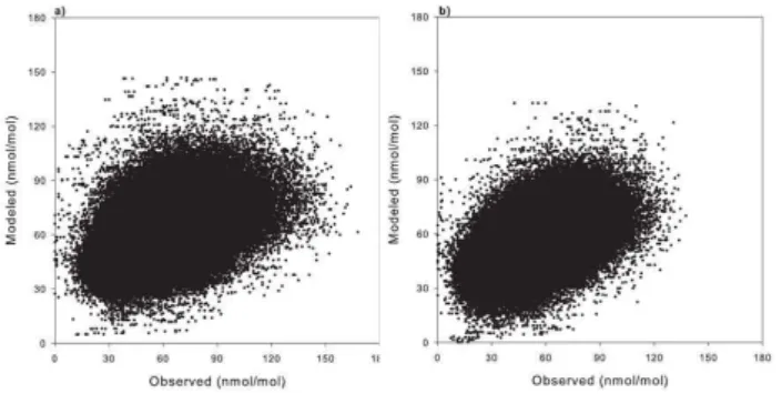
maximum mixing ratios at all sites within the model do-main during the five summers, the mean bias (OBS-MOD) was 0.7 nmol/mol (±17 nmol/mol), the root mean square er-ror (RMSE) 17 nmol/mol, index of agreement (IA) 69% and the correlation coefficient (r) between observations and mod-eled results was 0.51. The modmod-eled and observed 1-h O3 daily maxima at all monitoring sites from each day of the five summers were also plotted in a one-to-one correspond-ing manner (Fig. 4a). The slope value of this correlation was 0.37, resulting from overprediction of lowers values and un-derprediction of higher levels. Apparently, the small mean bias value does not necessarily mean close one-to-one agree-ment between observations and model results, which is re-flected in the standard deviation of the mean bias. On the contrary, it was a result of over- and under-predicted values cancelling each other. Current regional air quality models commonly produce similar order of agreement with observa-tions (e.g., Hogrefe et al., 2004; Zhang et al., 2006a; Otte, 2008; Vivanco et al., 2009).
One-hour O3 daily peaks averaged over the 2001–2005 summers from the EPA AIRNOW measurements show that south of the northern borders of Pennsylvania (PA), Ohio (OH), and Indiana (IN), mean 1-h O3daily maxima at most
stations exceeded 60 nmol/mol. The highest levels (70–75 nmol/mol) were found in neighboring areas of PA, New Jersey (NJ), Maryland (MD), Virginia (VA), and Delaware (DE) (Fig. 5a). An elongated patch of O3 mixing rations over 60–70 nmol/mol spanned mainly the middle of the do-main in a southwest-northeast orientation and a few smaller areas in the southwestern states (Fig. 5a). Lower values (<50 nmol/mol) occurred in Maine (ME), Wisconsin (WI), Minnesota (MN), and Iowa (IA).
Our model simulations captured the pattern and magni-tude of the observed salient features in the spatial distribu-tion of 1-h O3daily maxima with primary exceptions in Al-abama (AL) and Georgia (GA) as well as along the coast of the Mid-Atlantic States extending to southern New Eng-land, where modeled O3levels were higher than observations by 5–10 nmol/mol (Fig. 5b). Interestingly, the model simu-lations suggested higher O3 mixing ratios (>60 nmol/mol) over water than over land, i.e., the Great Lakes and off the east coast, possibly due to lower dry deposition and lower PBL height.
Table 1.Predominant map types for JJA from NCEP FNL and RCMS data sets and associated meteorological characteristics. The correlation
coefficient for map typing wasr=0.70.
Map Type Frequency Frequency Characteristics
FNL Types (%) RCMS Types (%)
Offshore anticyclone typically associated with the Bermuda High, warm and humid
FNL1 and RCM1 22 25 with general weak south-southwesterly
flow and weak subsidence over northeastern US, isolated rising motion associated with localized convection
Cold front off the coast with subsiding
FNL2 and RCM2 14 18 north-northwest flow inland,
cooling and clearing conditions
Cold front off the coast with subsiding north-northwest flow inland, cooling and
FNL3 6 – clearing conditions; similar to FNL2
except frontal trough further offshore and anticyclone extending further northeast producing more northerly – northeasterly flow
Anticyclone offshore retreating
FNL4 and RCM4 8 7 northeastward as cyclone approaches from
the west; general east to southeasterly flow in the northeastern US
Inland cold frontal trough extending from cyclone tracking across Canada
approaching the east coast, strong
south-FNL5 and RCM3 10 13 southwesterly warm, humid flow with
showers ahead of the front and cooler drier conditions and northwest flow over Midwest behind the front
Anticyclone centered near Hudson Bay extending into the northeastern US; cool,
FNL6 and RCM5 5 4 dry northerly flow over the coastal states
with warmer, humid, southerly flow over the Midwest states
Fig. 4.Modeled versus observed 1-h(a)and 8-h(b)O3daily max-imum mixing ratios.
compared to the latter. The model reproduced the general pattern and magnitude of the observed distribution (Fig. 5d). The overall mean bias was−0.4 nmol/mol (±14 nmol/mol), the RMSE 14 nmol/mol, and IA 71%. The observation-model r was 0.54 with a slope value of 0.39 (Fig. 4b), which is understandably slightly less scattered compared to the hourly data owing to the use of a moving average to ob-tain the 8-h data.
Table 2. Averaged observed (OBS) and modeled (MOD) 1-h O3 daily maximum mixing ratios (nmol/mol), difference (OBS-MOD) (nmol/mol) between the two, root mean square error (RMSE, nmol/mol), index of agreement (AINDEX, %), and the observation-model
correlation coefficient (R) from 480 monitoring sites over 4 June–31 August of 2001–2005.
Sample # OBS-MOD±σ OBS MOD RMSE AINDEX R
Daily 1-h O3Maxima
2001 55 718 2.3±17 62 60 17 68 0.48
2002 56 223 5.5±18 65 60 19 66 0.53
2003 57 300 1.7±15 59 57 15 70 0.52
2004 55 984 −3.6±15 52 56 15 64 0.46
2005 56 505 −2.5±17 58 61 17 71 0.51
Total 282 371 0.7±17 59 59 17 69 0.51
Daily 8-h O3Maxima
2001 55 718 1.8±14 55 53 14 73 0.58
2002 56 223 3.4±16 58 54 16 69 0.56
2003 57 300 −0.3±14 52 52 14 69 0.52
2004 55 984 −4.7±13 46 51 13 65 0.51
2005 56 505 −3.2±14 52 55 14 73 0.57
Total 282 371 −0.6±14 52 53 14 71 0.54
Fig. 5.Observed and modeled surface 1-h (aandb) and 8-h (cand
d) O3daily maxima averaged over summers 2001–2005.
In general smaller values occurred in the first and last two weeks of the season, and a biweekly cycle appeared to be embedded in the seasonality. The model captured these key features very well albeit with overprediction of dips and un-derprediction of peaks. In particular, the largest discrepancy (9 nmol/mol) between observations and model was found during the 23–27 June period when O3reached the seasonal maximum of 72 nmol/mol. This is illustrated in more detail at individual UNH AIRMAP sites in Sect. 5.1.
The over-/underprediction tendency of model simulations
6/1 6/16 7/1 7/16 7/31 8/15 8/30
O3
(n
m
o
l/mo
l)
40 50 60 70
Observed
Modeled
6/1 6/16 7/1 7/16 7/31 8/15 8/30
O3
(n
m
o
l/mo
l)
40 50 60 70
Observed
Modeled
b) 8h-O3
a) 1h-O3
Fig. 6.Domain and 5-summer averaged 1-h(a)and 8-h(b)O3daily maximum mixing ratios over June–August.
is represented distinctly in the cumulative distribution of in-stantaneous 1- and 8-h O3daily maxima from the entire do-main over all summers (Fig. 7). The model overpredicted ob-served 1-h O3daily peaks<56 nmol/mol by 0–9 nmol/mol, which comprised 47% of the total number of data points and underpredicted observed 1-h O3daily peaks>56 nmol/mol with the largest difference reaching 21 nmol/mol at the 100th percentile level (168 nmol/mol). This suggests that the model performed best in simulating moderately polluted conditions and less satisfactorily in highly polluted ones. The 8-h data showed under- and overprediction of close magnitude (∼10 nmol/mol) at the lower and upper end of the distribu-tion.
Fig. 7. Cumulative distributions of frequency of 1-h (solid) and
8-h (dotted) O3daily maxima from observations (red) and model
simulations (green).
Fig. 8.Distributions of frequency of 1-h and 8-h O3daily maxima for different bins from observations and model simulations.
Ambient Air Quality Standards (NAAQS) for 1-h O3 data. The model performed reasonably well in simulating the over-all distribution, with the peak frequency of occurrence in the same bin as observations. The predicted frequency in bins over 40–70 nmol/mol was larger than the observed by 3–8% whereas it was a factor of two smaller than the observed in the bins of <40 nmol/mol and >80 nmol/mol. Compared to 0.3% of the observed points being categorical O3 ex-ceedance, the model captured 0.05% of the total for that case, a factor of six smaller, which raises caution in using models to predict the areas of O3exceedance. The observed distribution of frequency of occurrence for averaged 8-h O3 daily peaks showed a decreasing trend from the lowest O3 bin to the highest with the largest frequency being 25% in the bin<40 nmol/mol. The model captured less than half of the frequency of occurrence in the bin<40 nmol/mol, over-predicted by∼10% in the bins 40–60 nmol/mol, predicted a value in close agreement with observations in the bin of 60–70 nmol/mol, and underpredicted significantly in the bins
>80 nmol/mol.
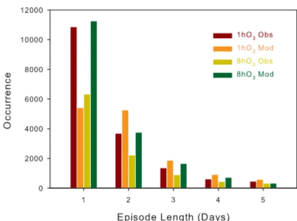
Fig. 9. Distributions of occurrence of episodes of varying length
using 1- and 8-h O3daily maxima from observations and model
simulations.
Another index to quantify air pollution is the length of an O3 episode; the longer an episode lasts the more likely a regional build-up of pollutant levels will occur. CMAQ’s tendency to underestimate higher O3levels can conceivably result in missing out those O3exeedance days that are defined by the NAAQS criterion from simulations, and can further underestimate the number of occurrences of O3episodes. To apply model results more meaningfully, as opposed to just using one single number as the universal exceedance crite-rion, we defined an exceedance to be when the O3daily max-imum level exceeded the 90th percentile value calculated for each monitoring site based on all daily maximums during the five summers, and we defined an episode to be a succession of days of such exceedances.
During the five summers there were 16 887 and 13 949 ex-ceedance occurrences across all monitoring sites in the 1-h O3daily maxima data of observations and simulations, re-spectively. The model underestimated the occurrence of O3 exceedance by 17%. We grouped the episodes into five cat-egories with length of one-to-four days at a one-day interval (Fig. 9). The model overestimated the occurrence of episodes in all length bins by 27–52% with the largest overestimation (∼52%) for the four-day episode type except the one-day group, for which the model underestimated episode occur-rence by 50%. The model captured episodes of three- and
>four-day episodes with the greatest accuracy. The 8-h O3 daily maxima data (Fig. 9) showed that the model overesti-mated all types even more significantly except for the> four-day type, in which the model was in close agreement with observations (2%).
4.2 Association between circulation and O3distribution
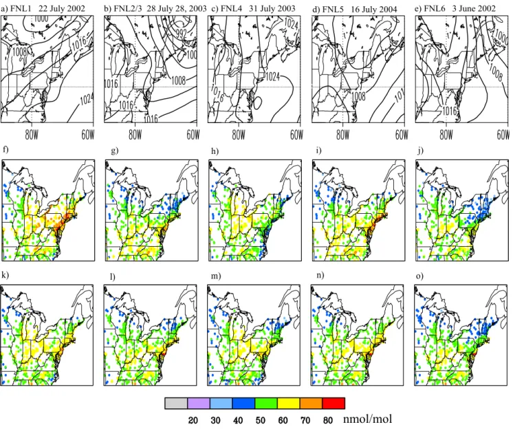
a) FNL1 22 July 2002 b) FNL2/3 28 July 28, 2003 c) FNL4 31 July 2003 d) FNL5 16 July 2004 e) FNL6 3 June 2002
f) g) h) i) j)
nmol/mol
k) l) m) n) o)
Fig. 10.The top 5 map types from reanalysis(a–e)and corresponding average distributions of 1-h O3daily maxima from observations(f–j) and model results(k–o).
and modeled average distribution of 1-h daily maximum O3 are presented in Fig. 10. The salient features in the observed average distribution corresponding to the five map types are very similar to those in Hegarty et al. (2007) where the re-lationship was investigated between synoptic-scale circula-tion patterns and surface O3across the northeastern US for summers 2000–2004. We found that FNL1 and FNL5 de-pict the two stages of cold front passage over the North-east with FNL1 preceding FNL5 (Fig. 10a and d). In these two map types, the Bermuda High prevailed over the east-ern US producing weather conditions with strong solar ra-diation and warm temperatures conducive to occurrence of high O3levels. Consequently, in these two map types higher O3 levels were observed across the eastern US before the cold front moved the polluted air offshore (Fig. 10f and i).
Map types FNL2 and FNL3 represent the stages where the cold front moved off of the continent with influx behind it of relative clean Canadian air into New England reduc-ing the O3 level in the region as revealed by observations (Fig. 10g). Lower O3 levels were observed along the east coastline (Fig. 10h) corresponding to the FNL4 circulation and in particular spread out extensively across the Northeast as shown in FNL6 (Fig. 10e and j). Map types FNL4 and FNL6 are not conducive to O3formation and build-up due to the influx of marine air and cool and dry Canadian air masses from over Hudson Bay respectively.
FNL5, while overestimation of lower levels was particularly apparent along the southeastern coastline in FNL4 and in New England in FNL2 and FNL3. Overall, capturing the pri-mary features of climatological circulation patterns appeared to be critical to simulating accurately surface O3mixing ra-tios.
5 Model comparison to observations
In this section only 1-h data were used for model and ob-servation comparison because the objective was to further evaluate model skill in representing chemical and dynami-cal processes. Hence we believe that the model-observation discrepancy for this purpose should be examined as is, rather than being mathematically smoothed to some extent due to the use of 8-h O3data.
In our previous episode studies (Mao et al., 2004, 2006) we used the AIRMAP ground-based and some of ICARTT multi-platform observations for model evaluation, which overlapped parts of the application of these observations in this study. In this study, in addition to capturing the overall seasonal variability in O3over the five summers, the model was also examined for its ability to reproduce the ensemble of particular episodes in the multi-season context. Thus the model-observation comparison conducted here is more ro-bust than episode studies, and consequently it can enhance our confidence in the model performance should the results be satisfactory.
5.1 AIRMAP ground-based observations
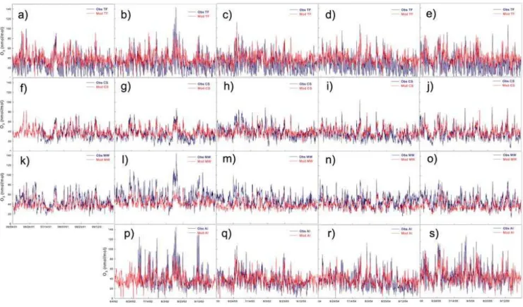
We compared modeled hourly O3 mixing ratios with ob-servations from the four AIRMAP sites, Thompson Farm (TF) (24 m a.g.l.), Castle Springs (CS) (320 m a.g.l.), Mount Washington (MW) (∼2 km a.g.l.), and Appledore Island (AI) (sea level) for all five summers with the exception of sum-mer 2001 for AI when measurements at that site were not yet available. Observations showed that median mixing ra-tios of O3at all four sites were similar except MW, at 28, 36, 33, and 45 nmol/mol for TF, AI, CS, and MW respectively, which suggests that the low elevation sites (<400 m) likely reflect the same regional airshed. In the time series of O3 mixing ratios at all sites showed a periodicity of 3–5 days (Fig. 11), which is possibly associated with synoptic scale dynamical processes.
Further, there are also distinct site idiosyncrasies due to their differing geographic characteristics. Our previous study suggested that the location of AI allows it to receive pol-luted air masses from more upwind source regions, such as the Mid-Atlantic States, the Greater Boston area, and/or the northeastern urban corridor, than inland New England sites (Mao and Talbot, 2004). This explains why AI was observed to experience higher O3levels more frequently than the in-land sites evidenced in its highest 90th percentile value of
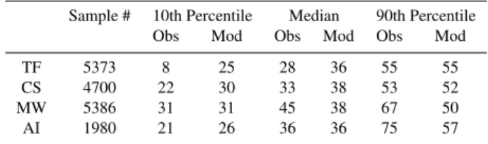
Table 3.AIRMAP sites.
Sample # 10th Percentile Median 90th Percentile
Obs Mod Obs Mod Obs Mod
TF 5373 8 25 28 36 55 55
CS 4700 22 30 33 38 53 52
MW 5386 31 31 45 38 67 50
AI 1980 21 26 36 36 75 57
75 nmol/mol compared to 55 and 53 nmol/mol at TF and CS respectively (Table 3). It is even higher than the 90th per-centile value of 67 nmol/mol at MW which often had en-hancements in O3levels due to free tropospheric and strato-spheric influences (Xiao et al., 2009). Specifically, over the five summers, there were 18 sample points at AI that ex-ceeded 120 nmol/mol, 3 at TF and MW, and none at CS.
The 10th percentile value at the coastal site TF was 8 nmol/mol, a factor of ∼3–4 lower than the other sites, which was driven by the low mixing ratios that were ob-served mostly on nights with the occurrence of a nocturnal inversion layer. These low values reached single digits and frequently zero for an extended period of hours on∼50% of summer nights (Talbot et al., 2005). Talbot et al. (2005) suggested that this phenomenon of nighttime depletion of surface O3was caused by continuous loss of surface O3via dry deposition and in situ chemistry with limited re-supply of O3-rich air masses from aloft.
CS is situated at an elevation of 320 m, near the top of the boundary layer at night, but in the middle of the convective boundary layer during the day. This characteristic determines that even on nights with the inversion layer, there is always exchange between the surface and the layers aloft. The loss of O3near the surface is thus constantly replenished, which is reflected in its lower 10th percentile value of 22 nmol/mol, almost a factor of 3 higher than at TF. At MW the lower 10th percentile and median values were larger than at CS and AI by∼10 nmol/mol and the 90th percentile value larger than at TF and CS by ∼13–14 nmol/mol but smaller than at AI by 8 nmol/mol. MW is frequently in the free troposphere, and hence observations suggest a mixture of influences on O3ranging from regional to farther upwind sources as well as stratospheric intrusions (Xiao et al., 2009).
Fig. 11.Time series of observed (blue) and modeled (red) 1-h O3daily maxima at the AIRMAP sites, Thompson Farm(a–e), Castle Spring
(f–j), Mount Washington(k–o)in summers 2001–2005 and Appledore Island(p–s)in summers 2002–2005.
We examined all nights with >30 nmol/mol overesti-mation, and averaged modeled and observed diurnal cy-cles including these nights (Fig. 12). Overprediction by
>30 nmol/mol at TF was mostly on nights with the observed occurrence of O3 depletion. However, instead of a steady decrease in O3 to near zero, modeled O3increased slightly from midnight to 05:00 LT followed by a∼5 nmol/mol de-crease during the next three hours. This indicates that in the model, there were source (s) for O3at night that likely included advection and/or exchange between the nighttime boundary layer and the residual layer aloft. We speculated that this may be due to misrepresentation of the nighttime boundary layer in the model, which was subsequently exam-ined.
The occurrence of nighttime O3depletion is a distinct in-dicator of the nocturnal boundary layer, which is depicted by minimal turbulence represented by small vertical eddy diffusivity (kzz) values in the model. Zhang et al. (2006b) suggested that the floor value ofkzz of 1.0 m2s−1 used in CMAQ v4.4 was too great causing over-mixing at night. Hu et al. (2003) showed that an optimal floor value ofkzzmay be between 0.1 and 1.0 m2s−1, and using a value of 0.1 m2s−1 reduced the positive normalized mean bias in modeled O3 mixing ratios by 16%. However, in our study the floorkzz value was reduced by a factor of 2 to 0.5 m2s−1, and it did not seem to effectively yield realistic nighttime O3
lev-els especially during depletion events. For example, during the period of 11–31 August 2001 our observations showed six nights with O3mixing ratios<5 nmol/mol. This clearly suggests the occurrence of the nocturnal inversion layer on those nights, and consequentlykzzshould be minimal. This was indeed captured in the model by implementation of the floor value ofkzz on those nights, and yet the model still overestimated O3 depletion by >30 nmol/mol. A separate model sensitivity study (Hwang et al., 2009) showed that the value ofkzz needed to be reduced to 10−4m2s−1to repro-duce the nighttime O3depletion, which is 3 orders of mag-nitude smaller than the lower end of the wide range (0.1– 5 m2s−1)reported/applied in literature (Hanna et al., 1982; Johansson and Janson, 1993; Plummer et al., 1996; Seifeld and Pandis, 1998; Stull, 1988; Zhang et al., 1982). It raises the possibility that the prescribed floor value ofkzzmay not be the dominant factor leading to nighttime overprediction of O3mixing ratios.
Local Time
00:00:00 06:00:00 12:00:00 18:00:00
O3
(
n
mol/mol)
0 20 40 60 80 100
Obs TF Mod TF Obs AI Mod AI
1
Fig. 12. Diurnal cycle of observed (dash) and modeled (solid)
1-h O3 daily maxima at Thompson Farm (red), and Appledore
Island (blue) averaged over days with nights of overestimation
>30 nmol/mol.
on average, which amounts to a contribution of 14 nmol/mol, or about 50% of that estimated by Talbot et al. (2005). This suggests that the model may underestimate O3titration by NO, which might have contributed to the considerable over-estimation of O3at night.
In comparison, the largest underestimation of O3 was found at AI in the window of 17:00–23:00 LT on days with a secondary daily maximum occurring at the site (Fig. 12). On average the observed O3mixing ratios reached their first peak at 14:00 LT and hovered around it for two hours. A secondary peak occurred at 18:00 LT followed by a slow de-crease during the next three hours and then dede-creased faster afterward. In comparison, the model depicted a textbook di-urnal cycle with the peak at 14:00–15:00 LT followed by a linear decrease over the next five hours. Mao and Talbot (2004) suggested that on days with favorable flow regimes and meteorological conditions conducive to O3 formation and buildup, it takes ∼4 h at an average wind speed of 6 m s−1 for air masses originating from the Greater Boston area to reach AI. In situ O3destruction/production likely oc-curs in air masses in transit between the two locations (Mao et al., 2006; Griffin et al., 2004; Pszenny et al., 2007). This can lead to a reprise after the peak hours of daytime O3levels at AI if the net production is positive, which was frequently observed in continental outflow from the Northeast (Mao et al., 2006). TF, a site just 25 km from AI and 10 km inland, was not likely receptive of air masses from such a transport route. However, the 36 km grid resolution is not fine enough to separate AI from TF; instead, the model treated the land use type of both sites as deciduous broad leaf vegetation, whereas in reality AI is situated completely in the marine boundary layer. We speculate that the misrepresented land use type and the subsequent incorrect simulation of
circula-tion and chemistry might have contributed to the missing of the secondary daily peak by the model.
Ozone daily maxima were most underpredicted at MWO likely due to three reasons. First, it is possible due to the no-flux upper boundary conditions at the model top (100 hPa), and thus the influence of stratosphere-tropospheric exchange was not taken into account properly in the model. IONS ozonesonde data suggested that the free troposphere over the northeastern North America was frequently enriched by stratospheric O3 during ICARTT 2004 (Thompson et al., 2007a) and that 20–25% of tropospheric O3 is of strato-spheric origin (Thompson et al., 2007b). Tang et al. (2009) showed much improved prediction of upper tropospheric O3 levels using the boundary conditions derived from IONS ozonesonde measurements. Second, this site can be recep-tive of influences from transboundary transport from south-ern Canada (DeBell et al., 2004a) and from as far away as Asia (DeBell et al., 2004b). In our model runs, the default boundary conditions in CMAQ were used, which means that O3mixing ratios on the boundaries were time-independent, which made it nearly impossible to represent accurately the impact of upstream source regions on the continental scale. Third, it may be the result of a mismatch in the model grid-averaged value and the observed value from a single point in the grid (Mao et al., 2006). Perhaps averaging the summit observations with those along the vertical slope of MW (not available) would make a more reasonable comparison with model results.
5.2 Model comparison with the duke forest intensive
The∼2-week O3 measurements at Duke Forest during the time period of 12–28 September 2004 showed an increas-ing trend in the daily maximum value over the first 12 days, reaching the highest 1-h O3 daily peak of 75 nmol/mol on 23 September followed by a decrease afterward (Fig. 13a). During that period, a high pressure system moved from southern Canada toward the northeastern US on 18 Septem-ber, stagnated with its center over OH and PA during 20– 23 September, and began weakening/moving off the coast on the 24th. The spatial distribution of 1-h O3daily peaks on 23 September showed pervasive higher O3 levels in the Northeast with highest patches (>80 nmol/mol) in OH, PA, Mid-Atlantic States, and southern Canada.
51
1
2
3
4
5
6
9/12/04 9/16/04 9/20/04 9/24/04 9/28/04
O3
(nmol/mol
)
0 20 40 60 80
Obs Duke
Mod Duke
9/15/04 9/17/04 9/19/04 9/21/04 9/23/04 9/25/04 9/27/04
W
in
d
S
p
ee
d (m
s
-1 )
0 2 4 6
8 Obs
Mod
b)
9/15/04 9/17/04 9/19/04 9/21/04 9/23/04 9/25/04 9/27/04
Tempera
ture
(C)
5 10 15 20 25 30
Obs
Mod
c)
a)
Fig. 13. Time series of modeled (red) and observed (blue) hourly O3(a), hourly wind speed(b), and temperature(c)at Duke Forest, NC during our campaign.
Further examinations of the results revealed that the model was far off as to accurately representing wind speed over the entire period except the few days, 22–24 September, with rel-ative higher O3mixing ratios and calm wind speed (Fig. 13a and b). The Duke site was influenced predominately by northerly to easterly winds during September 2004 with two excursions caused by the peripheral influence of Hurricanes Ivan (16 September) and Jeanne (26 September). Periods of elevated wind speeds are coincided with passing of the
storms as evidenced by the revolving nature of the wind rection over a two day interval. The disruption in the basic di-urnal cycles of O3and air temperature by the passage of these storms is readily apparent. For instance, in the 19 September reanalysis data the center of Hurricane Ivan was a few hun-dred kilometers offshore, and NC was under the influence of a ridge associated with the strong high pressure system centered in southern Canada (Fig. 14a). The modeled wind speed deviated the most from reanalysis on that day, as the simulated sea level pressure and wind vectors showed that Hurricane Ivan made landfall in NC (Fig. 14b). In compar-ison, during the period of 22–24 September the model per-formed well in capturing the dominance of the high over land in both position and magnitude and the approaching low in the west (Fig. 14c and d). This result again points to the im-perative requirement of reasonable simulation of circulation patterns in order to reproduce observed O3levels, as docu-mented here for Duke Forest.
5.3 Model-observation comparison during NEAQS 2002 and ICARTT 2004
Model results were also compared with a suite of NEAQS 2002 and ICART 2004 measurements from the NOAA ship
Ronald H. Brownand 2004 ozonesondes from the IONS net-work. Overall the modeled trends in O3during the two inten-sives agreed reasonably well as demonstrated by comparison to theRon Brown observations (Fig. 15). The model per-formed particularly well in capturing episodes of higher O3 mixing ratios, such as 15–20 July 2002, 22–23 July 2002, 3–6 August 2002, 9–14 July 2004, 20–23 July 2004, and 3– 4 August 2004. The three episodes of lower O3levels, 24– 27 July 2002, 5–8 July 2004, and 27 July–2 August 2004, were also depicted with reasonable agreement in magnitude compared to measurements.
Geographically, the model reproduced the west-east gra-dient in O3mixing ratios during NEAQS 2002 from higher values immediately offshore to lower ones farther out over water, and the latitudinal gradient of higher in the south near the North Carolina coast to lower in the northern states (as far north as Maine). It also simulated a few hot spots just offshore of the New York City and Boston metropolises (Fig. 16a and b). Similarly during ICARTT 2004 the modeled trend in O3along theRon Brown cruise tracks agreed well with shipboard observations, especially in the near-coastal areas northeast of Greater Boston and in southern ME (Fig. 16c and d). The lowest O3 mix-ing ratios (<30 nmol/mol) occurred in the near-coastal area east of Boston, and slightly higher levels of 40–50 nmol/mol
∼50 km farther out over the ocean. A scatter plot of mod-eled versus observed values showed a 1-to-1 correlation with
1
2
3
4
5
6
7
8
9
10
11
12
13
14
15
16
17
a)
c)
b)
d)
Fig. 14.Analyzed (aandc) and modeled (bandd) sea level pressure and wind vectors for 19 and 23 September 2004.
in agreement with the model evaluation in Mao et al. (2006) where they found accurate simulation of the position of the relatively high O3mixing ratios accompanied by consider-able underestimation of the absolute values of the channeled pollution. CMAQ seems to have an inherent problem in un-derpredicting O3levels in continental outflow, possibly due to underestimation of O3 precursors in the model and thus underprediction of in situ O3production during transport.
In addition to ground-level comparisons, we examined model performance in simulating upper air O3 mixing ra-tios using ozonesonde data obtained at three ICARTT-IONS locations in Narragansett, RI, Pellston, MI, Beltsville, MD, Huntsville, AL, Wallops Island, VA, and the ship
7/12/02 7/17/02 7/22/02 7/27/02 8/1/02 8/6/02 8/11/02
O3
(n
mol/mol)
0 20 40 60 80 100 120
Obs
Mod
7/6/04 7/11/04 7/16/04 7/21/04 7/26/04 7/31/04 8/5/04 8/10/04
O3
(
n
mo
l/mo
l)
0 20 40 60 80 100 120
Obs
Mod
a) NEAQS2002
b) ICARTT2004
Fig. 15.Time series of hourly O3from ship observations (blue) and
model results (red) in NEAQS 2002(a)and ICARTT 2004(b).
influences (Fig. 17a) (Pfister et al., 2008; Yorks et al., 2009). In comparison, the modeled vertical profile remained al-most constant from the surface to 10 km, varying within 5 nmol/mol and a standard deviation of∼10 nmol/mol. The model captured the vertical trend at all sites with deviation of around±15 nmol/mol from observation below 6 km except for theRon Brownand at Beltsville. TheRon Brown obser-vations showed an increasing trend in O3from 25 nmol/mol at 2 m to 109 nmol/mol at 10 km, whereas the model sim-ulated an increase from 44 nmol/mol at 2 m to a peak of 59 nmol/mol at 600 m followed by a gradual decrease to 3 km and then an increase to the top of the troposphere. The model reproduced the shape of the vertical profile over Beltsville with underprediction >14 nmol/mol at all levels reaching maximum values in the top layer.
In their study on evolution of ETA-CMAQ forecast model results using the IONS 2004 measurements, Yu et al. (2007) reproduced the O3 vertical profile well at low altitudes, especially at the Pellston site, similar to what is shown in this study. However, the authors revealed a consis-tent model overestimation above∼6 km due to the lateral boundary conditions derived by the Global Forecast System
Fig. 16. Hourly O3from ship observations (aandc) and model
results (bandd) in NEAQS 2002 (aandb) and ICARTT 2004 (c
andd).
(GFS) model and coarse model resolution in the free tro-posphere. To the contrary, Tarasick et al. (2007) suggested that that the prescribed top O3 lateral boundary condition in all model versions contributes significantly to the large O3 underpredictions in the middle and upper troposphere. In our study the lack of structure in the modeled vertical profile indicates that some key processes are missing in the model in addition to the lack of stratosphere-tropospheric ex-change. For instance, lightning NOxis not represented in the CMAQ version employed in this study. Cooper et al. (2009) suggested that more than 80% of summertime upper tropo-spheric NOxabove the eastern US is produced by lightning. This missing source of NOxin the upper troposphere could potentially result in model underestimation of O3mixing ra-tios in that region.
O3 (nmol/mol)
0 50 100 150 200 250
A lt it u de (k m ) 0 2 4 6 8 10 Mod Obs a) Average at all sites
b.) Beltsville, MD
0 50 100 150 200 250
Al ti tu d e ( k m ) 0 2 4 6 8 10 12 obs mod
c.) Hunstville, AL
0 50 100 150 200 250 0 2 4 6 8 10 12 obs mod
d.) Narragansett, RI
0 50 100 150 200 250 0 2 4 6 8 10 12 obs mod
e.) Pellston, MI
O3 (nmol/mol) 0 50 100 150 200 250
Altitu de (km ) 0 2 4 6 8 10 12 obs mod
g.) Wallops Island, VA
O3 (nmol/mol)
0 50 100 150 200 250 0 2 4 6 8 10 12 obs mod f.) Ron Brown
O3 (nmol/mol)
0 50 100 150 200 250 0 2 4 6 8 10 12 obs mod
Fig. 17.Vertical profiles of O3mixing ratios from IONS observations and model simulations during ICARTT 2004.
3 4 5 6 7 Observed
20 40 60 80 100 120 140 160 180
M o de le d 20 40 60 80 100
r2 = 0.23
mod = 43+0.19xobs
7/2/04 7/8/04 7/14/04 7/20/04 7/26/04 8/1/04 8/7/04 8/13/04 O3 (nm o l/ mol) 0 20 40 60 80 100 120 140 160 180 Obs Mod a) b)
O3 (nmol/mol)
20 40 60 80 100 120
A ltitude (km) 0 2 4 6 8 10 obs mod c)
Fig. 18. (a)Correlation,(b) time series, and(c)averaged
verti-cal profiles of modeled and Observed O3from INTEX A during
ICARTT 2004.
Mixing ratios>100 nmol/mol were observed on 2, 22 July, and 6–7 August, which were completely missed by the model. The ones >100 nmol/mol mostly occurred at alti-tudes>7 km (Fig. 18c) which are likely to be the result of stratospheric influence that cannot be captured by the model owing to the top lateral boundary conditions.
6 Summary
We have examined model performance in the five summer (2001–2005) simulations of regional climate and O3 mix-ing ratios usmix-ing long-term continuous measurements from US and Canadian Surface Hourly Observations, National Weather Service radiosondes, the EPA AIRNOW and UNH AIRMAP as well as data from field campaigns NEAQS 2002, ICARTT 2004, and our Duke Forest 2004 work. Our map typing analysis suggested that RCMS captured the patterns and frequency of dominant five map types with the best agreement for the two most dominant map types with the re-analysis data. The modeled distributions of surface O3daily maxima corresponding to these map types were in excellent agreement with observations. This suggests that accurate simulation of circulation was a deterministic factor in repro-ducing the salient features in surface O3 distribution. The mean bias, root mean square error, and index of agreement of the five summer modeled surface 8-h O3 daily maxima simulated by CMAQ, as compared to observations, were
Moreover, the diagnostic analysis suggested that signifi-cant overestimation of nighttime low O3 mixing ratios for the coastal site Thompson Farm may have resulted from un-derestimated NO emissions at night. The missing of the sec-ond daily peak at the marine site Appledore Island possibly resulted from the misrepresentation of land surface type of the site due to the coarse grid resolution. The comparison of modeled andRon Brownshipboard measurements from NEAQS 2002 and ICARTT 2004 suggested that CMAQ has an inherent problem in under-predicting O3levels in conti-nental outflow, probably due to underrepresented O3 precur-sor emissions in the model. While CMAQ appeared to sim-ulate the lower tropospheric O3distribution reasonably, the overall lack of structure in the modeled vertical profiles indi-cates that key processes missing in the model, such as light-ning produced NOxand stratospheric intrusions, are impor-tant for accurate free tropospheric simulations. Future work is warranted to improve the representation of O3 precursor emissions and processes influencing upper tropospheric air to better simulate the three-dimensional distribution of O3. Acknowledgements. We thank two referees’ constructive
comments. We thank Eric Williams and Brian Lerner of
NOAA/ESRL/CSD for the Ronald Brown O3measurements. We
thank T. Hagan’s assistance in model simulation and the help of C. Hogrefe with technical questions on SMOKE and CMAQ runs. This work was funded by the Environment Protection Agency
under STAR grant#RD-83145401 and the Office of Oceanic and
Atmospheric Research of the National Oceanic and Atmospheric
Administration under AIRMAP grant #NA06OAR4600189 to
UNH.
Edited by: R. Sander
References
Byun, D. W. and Schere, K. L.: Review of the governing equa-tions, computational algorithms, and other components of the Models-3 Community Multiscale Air Quality (CMAQ) Model-ing System, Applied Mechanics Reviews, American Society of Mechanical Engineers, Fairfield, NJ, 59(2), 51–77, 2006. Chai, T., Carmichael, G. R., Tang, Y., Sandu, A., Hardesty, M.,
Pilewskie, P., Whitlow, S., Browell, E. V., Avery, M. A., N´ed´elec, P., Merrill, J. T., Thompson, A. M., and Williams, E.: Four-dimensional data assimilation experiments with International Consortium for Atmospheric Research on Transport and Trans-formation ozone measurements, J. Geophys. Res., 112, D12S15, doi:10.1029/2006JD007763, 2007.
Changnon, S. A., Kunkel, K. E., and Reinke, B. C.: Impact and re-sponses to the 1995 heat wave: a call to action, B. Am. Meteorol. Soc., 77, 1497–1506, 1996.
Chen, M., Pollard, D., and Barron, E. J.: Regional climate change in East Asia Simulated by an interactive soil-vegetation-atmosphere model, J. Climate., 17, 557–572, 2004.
Chen, M., Mao, H., and Talbot, R.: Changes in precipitation
char-acteristics over North America for doubled CO2, Geophys. Res.
Lett., 32, L19716, doi:10.1029/2005GL024535, 2005.
Cooper, O. R., Eckhardt, S., Crawford, J. H., et al.:
Summer-time buildup and decay of lightning NOxand aged thunderstorm
outflow above North America, J. Geophys. Res., 114, D01101, doi:10.1029/2008JD010293, 2009.
Dawson, J. P., Racherla, P. N., Lynn, B. H., Adams, P. J., and Pandis, S. N.: Simulating present-day and future air quality as climate changes: Model evaluation, Atmos. Environ., 42(19), 4551–4566, 2008.
DeBell, L. J., Talbot, R. W., Dibb, J. E., Munger, J. W., Fis-cher, E. V., and Frolking, S. E.: A major regional air pollution event in the northeastern United States caused by extensive for-est fires in Quebec, Canada, J. Geophys. Res., 109, D19305, doi:10.1029/2004JD004840, 2004a.
DeBell, L. J., Vozzella, M., Talbot, R. W., and Dibb, J.
E.: Asian dust storm events of spring 2001 and
associ-ated pollutants observed in New England by the Atmospheric Investigation, Regional Modeling, Analysis and Prediction (AIRMAP) monitoring network, J. Geophys. Res., 109, D01304, doi:10.1029/2003JD003733, 2004b.
Dudhia, J.: Numerical study of convection observed during the winter monsoon experiment using a mesoscale two-dimensional model, J. Atmos. Sci., 46, 3077–3107, 1989.
Gery, M. W., Whitten, G. Z., Killus, J. P., and Dodge, M. C.: A photochemical kinetics mechanism for urban and regional scale computer modeling, J. Geophys. Res., 94, 12925–12956, 1989. Grell, G. A., Kuo, Y. H., and Pasch, R.: Semi-prognostic tests of
cumulus parameterization schemes in the middle latitudes, Mon. Weather Rev., 119, 5–31, 1991.
Griffin, R., Johnson, C., Talbot, R., Mao, H., Russo, R., Zhou, Y., and Sive, B.: Quantification of ozone formation metrics at Thompson Farm during NEAQS 2002, J. Geophys. Res., 109, D24302, doi:10.1029/2004JD005344, 2004.
Hanna, S. R., Briggs, G. A., and Hosker, R. P.: Handbook on At-mospheric Diffusion, Technol. Inf. Cent., US Dep. of Energy, Washington, DC, 1982.
Hegarty, J., Mao, H., and Talbot, R.: Synoptic influences on
spring-time tropospheric O3and CO over the North American export
region observed by TES, Atmos. Chem. Phys., 9, 3755–3776, 2009,
http://www.atmos-chem-phys.net/9/3755/2009/.
Hegarty, J., Mao, H., and Talbot, R.: Relationships
be-tween circulation patterns and surface ozone over the
North-eastern United States, J. Geophys. Res., 112, D14306,
doi:10.1029/2006JD008170, 2007.
Hogrefe, C., Biswas, J., Lynn, B., Civerolo, K., Ku, J.-Y., Rosen-thal, J., Rosenzweig, C., Goldberg, R., and Kinney, P. L.: Sim-ulating regional-scale ozone climatology over the eastern United States: model evaluation results, Atmos. Environ., 38, 2627– 2638, 2004.
Hong, S.-Y. and Pan, H.-L.: Nonlocal boundary layer vertical dif-fusion in a medium-range forecast model, Mon. Weather Rev., 124(10), 2322–2339, 1996.
Huang, H.-C., Liang, X.-Z., Kunkel, K. E., Caughey, M., and Williams, A.: Seasonal simulation of tropospheric ozone over the Midwestern and Northeastern United States: An application of a coupled regional climate and air quality modeling system, J. Appl. Meteorol. Clim., 46, 945–960, 2007.
Phys. Discuss., in preparation, 2009.
Johansson, C. and Janson, R. W.: Diurnal cycle of monoterpenes in a coniferous forest: Importance of atmospheric stability, sur-face exchange, and chemistry, J. Geophys. Res., 98, 5121–5133, 1993.
Liang, X.-Z., Li, L., Kunkel, K. E., Ting, M., Wang, J. X. L.: Regional climate model simulation of US precipitation during 1982–2002. Part I: annual cycle, J. Climate., 17(18), 3510–3529, 2004.
Lund, I. A.: Map-pattern classification by statistical methods, J. Appl. Meteorol., 2, 56–65, 1963.
Mao, H. and Talbot, R.: The role of meteorological processes in two New England ozone episodes during summer 2001, J. Geophys. Res., 109, D20305, doi:10.1029/2004JD004850, 2004.
Mao, H., Talbot, R., Troop, D., Johnson, R., Businger, S., and Thompson, A. M.: Smart balloon observations over the North
Atlantic: O3data analysis and modeling, J. Geophys. Res., 111,
D23S56, doi:10.1029/2005JD006507, 2006.
Mena-Carrasco, M., Tang, Y., Carmichael, G. R., et al.: Im-proving regional ozone modeling through systematic evalua-tion of errors using the aircraft observaevalua-tions during the In-ternational Consortium for Atmospheric Research on Trans-port and Transformation, J. Geophys. Res., 112, D12S19, doi:10.1029/2006JD007762, 2007.
New England Regional Assessment Group, Preparing for a chang-ing climate: The potential consequences of climate variabil-ity and change, New England Regional Overview, US Global Change Research Program, University of New Hampshire, 96 pp., 2001.
Otte, T. L.: The impact of nudging in the meteorological model for retrospective air quality simulations. Part I: Evaluation against national observational networks, J. Appl. Meteorol. Clim., 47, 1853–1867, 2008.
Pfister, G. G., Emmons, L. K., Hess, P. G., Lamarque, J.-F., Thompson, A. M., and Yorks, J. E.: Analysis of the Sum-mer 2004 ozone budget over the United States using Inter-continental Transport Experiment Ozonesonde Network Study (IONS) observations and Model of Ozone and Related Trac-ers (MOZART-4) simulations, J. Geophys. Res., 113, D23306, doi:10.1029/2008JD010190, 2008.
Plummer, D. A., McConnell, J. C., Shepson, P. B., Hastie, D. R., and Niki, H.: Modeling of ozone formation at a rural site in southern Ontario, Atmos. Environ., 30(12), 2195–2217, 1996. Pollard, D. and Thompson, S. L.: Use of land-surface-transfer
scheme (LSX) in a global climate model: the response to dou-bling stomatal resistance, Global Planet. Change, 10, 129–161, 1995.
Pszenny, A. A. P., Fischer, E. V., Russo, R. S., Sive, B. C., and Varner, R. K.: Estimates of Cl atom concentrations and hy-drocarbon kinetic reactivity in surface air at Appledore Island, Maine (USA), during International Consortium for Atmospheric Research on Transport and Transformation/Chemistry of Halo-gens at the Isles of Shoals, J. Geophys. Res., 112, D10S13, doi:10.1029/2006JD007725, 2007.
Pierce, R. B., Schaack, T., Al-Saadi, J. A., et al.: Chemical data assimilation estimates of continental US ozone and ni-trogen budgets during the Intercontinental Chemical Transport Experiment-North America, J. Geophys. Res., 112, D12S21, doi:10.1029/2006JD007722, 2007.
Seinfeld, J. H. and Pandis, S. N.: Atmospheric Chemistry and Physics: From Air Pollution to Climate Change, John Wiley, New York, 1998.
Stull, R. B.: An Introduction to Boundary Layer Meteorology, 499– 541, Kluwer Acad., Norwell, Mass., 1988.
Talbot, R., Mao, H., and Sive, B.: Diurnal characteristics of
surface-level O3and other important trace gases in New England, J.
Geo-phys. Res., 110, D09307, doi:10.1029/2004JD005449, 2005. Tang, Y., Lee, P., Tsidulko, M., et al.: The impact of chemical
lat-eral boundary conditions on CMAQ predictions of tropospheric ozone over the continental United States, Environ. Fluid Mech., 9, 43–58, doi:10.1007/s10652-008-9092-5, 2009.
Tarasick, D. W., Moran, M. D., Thompson, A. M., et al.: Comparison of Canadian air quality forecast models with tropospheric ozone profile measurements above midlatitude
North America during the IONS/ICARTT campaign:
Evi-dence for stratospheric input, J. Geophys. Res., 112, D12S22, doi:10.1029/2006JD007782, 2007.
Thompson, A. M., Stone, J. B., Witte, J. C., et al.:
In-tercontinental Chemical Transport Experiment Ozonesonde
Network Study (IONS, 2004): 1. Summertime UT/LS
(Upper Troposphere/Lower Stratosphere) ozone over north-eastern North America, J. Geophys. Res., 112, D12S12, doi:10.1029/2006JD007441, 2007a.
Thompson, A. M., Stone, J. B., Witte, J. C., et al.: Intercontinen-tal Chemical Transport Experiment Ozonesonde Network Study (IONS) 2004: 2. Tropospheric ozone budgets and variability over northeastern North America, J. Geophys. Res., 112, D12S13, doi:10.1029/2006JD007670., 2007b.
Van Loon, M., Vautard, R., Schaap, M., et al.: Evaluation of long-term ozone simulations from seven regional air quality models and their ensemble, Atmos. Environ., 41, 2083–2097, 2007. Vincent, L. A., Wijngaarden, W., and Hopkinson, R.: Surface
Tem-perature and Humidity Trends in Canada for 1953–2005, J. Cli-mate, 20, 5100–5113, 2007.
Vivanco, M. G., Palomino, I., Vautard, R., Bessagnet, B., Mart´ın, F., Menut, L., and Jim´enez, S.: Multi-year assessment of pho-tochemical air quality simulation over Spain, Environ. Model. Software, 24, 63–73, 2009.
Xiao, Y., Mao, H., and Talbot, R.: Interannual variability of winter-spring ozone in the Northeastern US, Atmos. Chem. Phys. Dis-cuss., in preparation, 2009.
Yorks, J. E., Thompson, A. M., Joseph, E., and Miller, S. K.: The variability of free tropospheric ozone over Beltsville, Mary-land (39N, 77W) in the summers 2004–2007, Atmos. Environ., 43(11), 1827–1838, 2009.
Yu, S., Mathur, R., Schere, K., Kang, D., Pleim, J., Otte, T. L.: A de-tailed evaluation of the Eta-CMAQ forecast model performance for O3, its related precursors, and meteorological parameters dur-ing the 2004 ICARTT study, J. Geophys. Res., 112, D12S14, doi:10.1029/2006JD007715, 2007.
Yu, Y., Sokhi, R. S., Kitwiroon, N., Middleton, D. R., and Fisher, B.: Performance characteristics of MM5-SMOKE-CMAQ for a summer photochemical episode in southeast England, UK, At-mos. Environ., 42, 4870–4883, 2008.
Zhang, Y., Liu, P., Queen, A., Misenis, C., Pun, B., Seigneur, C., and Wu, S.-Y.: A comprehensive performance evaluation of MM5-CMAQ for the summer 1999 Southern Oxidants Study episode – Part II: Gas and aerosol predictions, Atmos. Environ., 40, 4839–4855, 2006a.