with an application to the predictability of
US interest rates using the term structure
Michael P. Clements Department of Economics
University of Warwick [email protected]
July 2001
Abstract
Ana Beatriz Galvão* Department of Economics
University of Warwick [email protected]
We evaluate the forecasting performance of a number of systems models of US short-and long-term interest rates. Non-linearities, induding asymmetries in the adjustment to equilibrium, are shown to result in more accurate short horizon forecasts. We find that both long and short rates respond to disequilibria in the spread in certain circumstances, which would not be evident from linear representations or from single-equation analyses of the short-term interest rate.
JEL Classification: C52, C53, E43.
1
Introduction
In this paper we test whether there are non-linearities in the response of short and long-term interest rates to the spread in interest rates. The simple Expectations theory of the term structure entails that the spread has significant predictive content in a linear framework, although there are reasons to expect non-linearities in the responses. We test for non-linearities and asymmetric adjustment using a variety of models and approaches, and carry out a number of forecast comparisons of the out-of-sample predictability of short and long-term interest rates using linear and non-linear models.
Existing studies have focused on possible asymmetries in the response of the short rate to positive and negative spreads, within a single-equation framework. We take as our starting point a systems approach, and show how single-equation techniques for testing and specification can be adapted. A systems approach allows proper ex ante forecasts of short- and long-term rates, and therefore also of the spread. This may be important for a variety of reasons, not least that interest rates, and especially spreads, have been found to be give advance warning of recessions in the US (see, inter alia, Estrella and Mishkin, 1998; Hamilton and Kim, 2000; Anderson and Vahid, 2000). We also consider the extent to which the implied patterns of adjustment are consistent with the expectations theory of the term structure of interest rates. In the
'Financiai support from the UK Economic and Social Research Council under grant L138251009 is gratefully acknowledged by the first author, and from Capes-Brazil by the second author. We are grateful to Dick van Dijk for helpful comments. This paper is based on chapter 2 of the PhD thesis of the second author. The computations reported in this paper were performed using code written in the Gauss Programming Language.
remainder of this introduction we provide a brief motivation, and discuss some aspects of the recent literature that we address.
A number of authors have investigated the effects of 'linear' cointegration on fore-cast performance in linear systems (see Clements and Hendry, 1995 and Christoffersen and Diebold, 1998, and the references therein). The inclusion of cointegration especially improves forecasts of cointegrating combinations of the variables. However, the linearity assumption may be too restrictive when, for example, there are transactions costs, so that arbitrage opportunit-ies between two markets only arise when the price differential is large enough to imply net gains to traders. In general, the speed of adjustment to equilibrium may depend on both the sign and size of the disequilibria. Moreover, some economic policies may affect the adjustment to equi-librium (Rudebusch, 1995; Roberds et aI., 1996), suggesting a non-linear adjustment processo Non-linear equilibrium correction models have been used to model the relationship between spot and future prices (Dwyer et aI., 1996; Martens et aI., 1998; Tsay, 1998), and between interest rates of different maturities (Anderson, 1997; Tsay, 1998; Enders and Granger, 1998; van Dijk and Franses, 2000).
A common finding of a number of recent papers that have considered the effects of non-linearities on economic forecasting in univariate models (e.g., Tiao and Tsay, 1994; Clements and Krolzig, 1998; Rothman, 1998; Montgomery et aI., 1998; Stock and Watson, 1999; Lundbergh and Terasvirta, 2000) is that a superior in-sample fit often fails to translate into out-of-sample forecast gains of a similar magnitude: see also Ramsey (1996). For example, after an evaluation of the forecast performance of univariate non-linear mo deIs applied to a large number of mac-roeconomic series, Stock and Watson (1999) concluded that in the majority of cases forecasts were worse than those of linear models.
Given that cointegration may improve forecasts in linear cointegrated systems, depending on how forecasts are evaluated, and that the improvements in forecasting from allowing for non-linearities in univariate mo deIs are on balance rather disappointing, the question we address in this paper is whether allowing non-linearities in the adjustment process in cointegrated systems is beneficiaI. We consider non-linearities in the term structure of interest rates, which has been a focus in the literature for much of the work on non-linear cointegration, and threshold vector equilibrium correction models (TVECMs). We evaluate the forecast performance of a number of non-linear systems of short and long-term US interest rates based on mo deis proposed in the literature (see, e.g., Anderson, 1997; Tsay, 1998; van Dijk and Franses, 2000). Our models are specified and tested using recently developed techniques, as described in section 3.
The three main contributions of our paper are: to provide a review of the econometric tests of non-linear cointegration, and extensions to systems frameworks; to apply these tests to the US term structure of interest rates; and to assess any gains in out-of-sample predictability from allowing for non-linearities.
2 Term structure of interest rates and equilibrium correction
models
The Expectations Theory implies that at period t, the return on a k-period asset is the average of the current and a sequence of expected one period yields over the same period, t to t
+
k,plus a term premium:
(1)
rt(k) is the yield at maturity k; Et is the expected value at time t; Lt is the term premium. The term premium consists of risk and liquidity premia. Assuming that yields are integrated of order one (1(1)), the possibility of the yield spread being cointegrated follows from rewriting
(1) as:
(2)
In the absence of Lt (k), the RHS of (2) will be I (O), consisting of a finite sum of 1 (O) components (the .0.rt+j(l)). Then each yield rt(k) is cointegrated with rt(l), and the spreads are stationary, so that spreads between any two yields will be 1 (O) ( Hall et aI., 1992). It follows that a Vector Equilibrium Correction Model (VECM) for any two yields, say, a short-term (s) and long-term (l) yield, can be written as:
.0.rt = c(L).0.rt-l - a(St-l - p,)
+
ét (3) where rt = [rt(s), rt(l)]'; c(L) is a matrix of coefficients in the lag operator; St = rt(l) - rt(s) isthe spread; p, is the equilibrium spread; a is the adjustment vector to the long-run attractor; and ét is the vector of disturbances. L is the lag operator, LnXt
=
Xt-n, and .0.=
1 - L is the difference operator. Yields of different maturities can move apart in the short-run, but in the long-run are 'tied together'. p, may be different from zero because of a risk premium.The empirical evidence of cointegration between yields of different maturities, and the abil-ity of the ECM to improve forecasts of interest rates, is contested in the literature (Pagan et aI., 1996). The usefulness of the spread to forecast short-term rates is found to depend on the maturities (Rudebusch, 1995) and on the monetary policy in operation (Mankiw and Miron, 1986; Rudebusch, 1995; Roberds et aI., 1996; Gray, 1996). Tzavalis and Wickens (1998) note that the presence of time-varying risk premia in (3) may mask the predictive power of the spread, and in addition, the dynamics of .0.r (s) may depend on its leveI, as in the regime-switching mo deIs considered by Pfann et aI. (1996). Moreover, the Expectations Theory ig-nores transaction cost effects. These considerations - the diversity of monetary policies, the risk premium and the presence of transaction costs - can be accommodated in a non-linear equilibrium correction model, where the speed of adjustment to equilibrium depends on the regime.
is no adjustment, where asymmetry arises if Tl
=I-
Tu. Outside this band, adjustment may occurat different speeds. 8upposing that individual investors have different transaction costs implies that in the aggregate the effect of transaction costs might be smooth, leading to the Smooth Transition Equilibrium Correction model (STEqCM): see Anderson (1997) and van Dijk and Franses (2000). Both these applications are single-equation analyses, although van Dijk (1999, ch. 5, p. 128) discusses bivariate STVECMs (Smooth Transition Vector Equilibrium Correction models).
3 ThreshoId vector equilibrium correction modeIs
In this section we discuss aspects of testing, mo deI specification and estimation procedures for non-linear equilibrium correction models.
3.1 Non-linearity testing
Threshold vector equilibrium correction models are extensions of univariate Threshold Autore-gressive (TAR) mo deIs (see, e.g., Tong, 1995), and inherit the non-standard aspects of testing for non-linearity that arise from the presence of nuisance parameters under the null when likelihood-based approaches are used (see, e.g., Ransen, 1996).
The benchmark mo deI is a linear VECM of the form of (3) (the change in notation is to aid comparison with the non-linear models that follow):
p
l::;.rt
=
c+
L
cI>l,jl::;.rt-j+
aSt-l+
ct, j=1(4)
where the autoregressive order p is set to minimize an information criteria. A possible non-linear alternative hypothesis is that interest rates follow a threshold VECM (TVECM), such that:
p
l::;.rt = c;,
+
L
cI>i,jl::;.rt-j+
ai S t-1+
Eit j=1(5)
if ri-1
<
Zt-d ::; ri, where i=
1,2 in the case of a two-regime model (with ro=
-00,
r2=
+00)
and i=
1,2,3 for a three-regime model (with ro=
-00,
r3=
+00),
and {Ci, cI>i,j,ad
depend on the regime i. Zt-d is the transition variable with delay d; ri are the thresholds; and ai is (2 xl), allowing the spread to enter as an explanatory variable in both equations. The i subscript on Et indicates that the covariance matrix of the disturbances may depend upon the regime.3.1.1 Tsay (1998)
regression. The test is constructed by regressing the (standardized) predictive residuaIs on the explanatory variables, and testing for the significance of the latter: see Tsay (1998, p. 1189 -1191), for details. The simulation results presented by Tsay (1998) indicate that this test has good power when d is correctly specified.
3.1.2 Balke and Fomby (1997)
Balke and Fomby (1997) proposed a two step procedure to test non-linearity in cointegrated systems. The first step is to test for cointegration using a standard method, such as OL8 and an ADF test, as in Engle and Granger (1987), or the Johansen ML procedure, Johansen (1988). The second step tests for non-linearity in the cointegrating combination, using a test of linearity against 8ETAR structure, such as Hansen (1996, 2000). An asymptotic approximation to the p-value of the null of linearity (or of a 2-regime versus a 3-regime structure) can be obtained by simulation, or a small-sample approximation can be calculated by bootstrapping.
3.1.3 Enders and Granger (1998) and Enders and Siklos (2001)
Testing for cointegration (as in of 8tep 1 of Balke and Fomby (1997) above) may have low power when the process is I (O) but exhibits non-linear mean reversion: see, e.g., the Monte Carlo evidence in Balke and Fomby (1997). Enders and Granger (1998) proposed a test for a unit root in a series against asymmetric adjustment under the alternative hypothesis, whereby the process is either a two-regime TAR or an M-TAR (Momentum-TAR). For the former, the rate of autoregressive decay depends on whether the variable is above or below some threshold, and for the latter, on whether the variable is increasing or decreasing. For example, when the threshold is zero, the following regression is run:
(6) where, for the TAR alternative, It
=
1 if St-l2::
O, and is zero otherwise, and for testing against the M-TAR alyternative, It = 1 if f.}.St-l2::
O, and is zero otherwise. Enders andGranger obtain by simulation criticaI values for the unit root null that Pl = P2 = O against both these alternatives, and for various modifications of the above set up (e.g., when the attractor is not zero, but has to be estimated, and when lagged f.}.St terms are added in the event that the estimated error, Êt, exhibits autocorrelation). Conditional on rejecting the null and finding Pl
<
O and P2<
O, tests that Pl = P2 have standard distributions. Enders and8iklos (2001) generalise these ideas to tests for cointegration, that is, when the variable is an estimated residual from an Engle-Granger static regression of one integrated variable on another (or several). In the case of the term structure, the residual is Wt = rt(l) - êrt(s) -
p,
where(ê,
p)
are OL8 estimates. The null hypothesis is now interpreted as a test that r (l) and r (s)zero for Wt). An incorrect assumption concerning the threshold would reduce the power of the test, but we do not pursue this as it turns out that we are able to reject the null against both alternatives.
3.1.4 A generalization of Hansen (2000)
Instead of testing St (or an estimated cointegrating relationship between r (l) and r (s» for non-linearity as outlined above, threshold effects can be tested for by comparing the linear system (4) against the non-linear alternative (5). This requires a multivariate extension of Ransen (2000). Imposing the restriction that the error covariance matrices are the same for the different regimes, the two- and three-regime TVECMs can be written as:
!:lrt [C1
+
t
<I>l,j!:lrt-j+
Ct1St-1] Glt (r1, r2)+
[C2+
t
iI>2,j!:lrt-j+
Ct2St-1] G2t(r1, r2)J=l J=l
+
[C3+
t
<I>3,j!:lrt-j+
Ct3St-1] G3t(r1, r2)+
U3t J=lwhere llt(r)
=
l(St-1 ::; r), b(r)=
l(St-1>
r)=
1 - llt(r), Glt (rI, r2)=
l(St-1 ::; rd,G2t (rI, r2)
=
l(r1<
St-1 ::; r2) and G3t (rI, r2)=
l(St-1>
r2), and l(·) is the indicator function. We denote the estimated covariance matrices of U2t and U3t byn
2 andn
3 , and letn
1 be the covariance matrix of the VECM1 . An LR test for linearity against the two-regimespecification is:
(7)
where T is the number of observations effectively employed in the estimation.
The asymptotic distribution is an extension of Ransen (1996), as argued by Ransen and Seo (2000). The bootstrap can be used to obtain a finite sample approximation. The bootstrap distribution is calculated from data generated by the linear mo deI by re-sampling its residuaIs. The residuaIs are corrected for heteroscedasticity before re-sampling, using a regression of the squared residuaIs on the squared regressors, as described in Ransen (2000).
A similar procedure can be applied to test linearity against the three-regime alternative:
(8)
or the two-regime versus the three-regime model.
3.1.5 Hansen and Seo (2000)
Rather than firstly estimating the cointegrating relationship, Ransen and Seo (2000) suggest a single step approach that jointly estimates the cointegrating vector and the defining
istics of the regimes. The non-linear mo deI is:
!!.r,
セ@
["+
t,
iI\',j!!.rl-j+
"'WH10)]
dulO, r)+ [" +
t,
il\2,j!!.rl-j+
a2W1-l(0)]
d,,(O, r)+
u,
(9)
where Wt(8) = rt(l) - 8rt(s) is the equilibrium correction term, dlt(8, r) = I(Wt-i(8)
S
r) andd2t(8, r) = I(Wt-i (8)
>
r). Their method involves estimating (9) at each point in a suitable gridof values defined over both 8 and r, and choosing the pair
(iJ,
f)
that minimizes log 1n
(8, r) 1(where
n
is the estimated residual covariance matrix). In practise, because of the limitations of the estimation by grid search, the delay is given, and the TVECM is restricted to having two regimes, as above. The authors also proposed an 'LM-like' non-linearity testo LM tests are calculated of the linear model against (9) with 8 =iJ,
the MLE in the linear VECM, and wherer takes on each of a pre-assigned set of values in the interval (rL, ru) (such that a minimum number of observations occur in each regime, say 10%). The test statistic is the supremum:
SupLM = sup LM(iJ, r). (10)
rL:S;r:::;ru
Hansen and Seo (2000) derive the asymptotic distribution of this statistic, and propose a boot-strap procedure to obtain a finite sample approximation.
3.2 Estimation
Tsay (1998) considers estimation of the TVECM by conditional multivariate least squares assuming the number of regimes, the autoregressive order p, and the threshold variable Zt are known. Equation (5) is estimated for alI permissible combinations of the delay d and the thresholds ri and r2 (for the 3-regime model), subject to a minimum number of observations in each regime, r2
>
ri, and d being a low integer. The estimates of the thresholds and dare3.3 Model specification
The choice of the threshold variable will usually be suggested by subject-matter considerations. The number of regimes of the TVECM may be selected based on theoretical considerations (as in e.g., Krager and Kugler, 1993 and Anderson, 1997), but as discussed in section 2, in the context of the term structure theoretical arguments can be put forward to support both two and three-regime mo deIs (respectively, adjustment depends upon whether the yield curve is normal or inverted, and transaction costs). Tests can be employed to determine whether there are two or three regimes, as for example the Hansen (2000) test for a two-regime versus a three-regime SETAR. We also use a systems generalization: the LR23 test that compares two-with three-regime TVECMs. In addition, Tsay (1998) suggests that the number of regimes s
may be selected along with the lag order p by using the AIC:
s
AIC =
L
[Tj In(IDjl)
+
2k(kp+
1)] ,
(11) j=lwhere k = 2 in the bivariate system,
Dj
is the estimated residual covariance matrix of regime j, and Tj is the number of observations in regime j. Thus the AIC is calculated for each combination of the threshold values, the delay and for s=
2,3, given that p=
2 for the models estimated in this work. Specific tests may also indicate the type of non-linear mo deI required. For example, the Enders and Granger (1998) and Enders and Siklos (2001) tests may suggest either TAR or MTAR.4 The evaluation of forecast performance
The models are compared on out-of-sample forecast accuracy as judged by their mean squared forecast errors at various horizons. We test whether differences between models are significantly different, and also calculate forecast encompassing tests.
Clements and Hendry (1995) and Christoffersen and Diebold (1998) find that there is a gain in forecast accuracyat longer horizons when the evaluation includes the ability to predict the cointegrating combination (here, the spread). Clements and Hendry (1993) show why forecast evaluation using the standard (root) mean squared forecast error criterion, (R)MSFE, may depend on the transformation of the variables adopted (e.g., the leveIs of the original variables, their first differences or growth rates, or a mixture of first differences and stationary combinations). Of interest here are forecasts of both interest rates and the spread, so we consider these separately for the most parto We look at forecasts of the differ,ences of the interest rates as these should be stationary. The MSFE for the variable x at horizon h is denoted by MSFEx,h,
and is calculated by averaging the squares of the h-step ahead forecast errors over a number of forecast origins, T. The MSFEs could be summed for the two rates, for example, to give the trace MSFE, TMSFE, as an estimate of the trace of the MSFE matrix. Rather than doing this, we report an overall measure of systems performance referred to as the GFESM by Clements and Hendry (1993), because this is invariant to whether we evaluate the mo deIs in terms of
d t = ei,t 2 - ej,t 2
ADM =
[n
+
1 -
2h+n n-
1h(h -1)]
1/2 DM (12)where t = 1, ... , n indexes the n h-step ahead forecasts that are available, and i and j index
the two models. So ei,t is the error in forecasting the value at t, made at t - h, using model i.
d
is the sample mean of the loss differential dt , where loss is symmetric, defined in terms of the squares of the errors. The estimated variance of the sample mean is denoted by V(d), and depends on the sample autocovariances of dto Under the null of equal forecast accuracy, DM is asymptotically standard normal. Thus values of the statistic in the left tail suggest model i is more accurate, and values in the right tail that j is more accurate. Harvey et aI. (1997) suggest comparing the Augmented Diebold and Mariano (ADM) test to the t-distribution to reduce size distortions, and Clark (1999) confirms that these modifications improve the small-sample performance of the testoWe can test whether mo deI i forecast encompasses mo deI j, that is, whether once we have mo deI i, there is any useful additional information contained in the forecasts of model j, by
modifying dt to:
(13)
Harvey et al., 1998 show that this test is equivalent to the forecast encompassing test of Chong and Hendry (1986): see Newbold and Harvey (2001) for a review. The condition that a mo deI forecast encompasses another is more stringent than that the mo deI is more accurate on the DM testo One mo deI may be more accurate than another on DM, but nevertheless, the dominated model contain useful information not incorporated in the superior model.
West (1996) and West and McCracken (1998) draw attention to the impact of parameter uncertainty on the size of the tests of equal forecast accuracy and encompassing, which is enhanced when the mo deIs are nested (Clark and McCraken, 2000). By ascribing a reasonable proportion of the observations to the in-sample, model estimation period, we hope it will be of secondary importance here.
5
Model estimates
The various TVECMs we employ are described in Table 1. They differ with regard to the testing, estimation or specification procedures used. We analyse the three month treasury bill at secondary market rate (r (3)) and the 10 year treasury constant maturity rate (r (120)),
5.1 Testing and rnodelling
Applying the procedures for specification of TVECMs outlined in section 3, we estimated five TVECMs (3 with 2 regimes, 2 with 3 regimes), as described in Table 12. For all models, p = 2, which minimizes the SIC for the linear VECM (the first mo deI in table 1). For the non-linear models, we set d = 1, folIowing, e.g., Anderson (1997) and Ransen and Seo (2000), but this
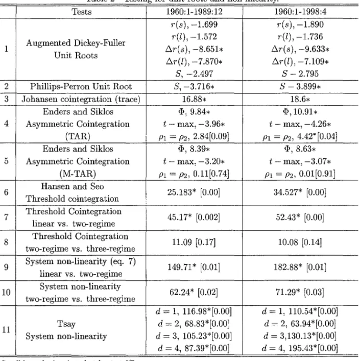
assumption is confirmed by the Tsay test presented in panel 11 of Table 2. The threshold(s) are calculated by a grid search, ensuring a minimum of 10% of the observations are in each regime.
For alI but two of the mo deIs the spread (St = r(l) - r(s)) is imposed as the equilibrium
correction term, and is used as the threshold variable. Table 2 panel1 indicates that r (l) and
r (s) are integrated of order 1 on the basis of ADF tests. There is some ambiguity over the spread: on the basis of an ADF test it is 1 (1), the Phillips-Perron tests indicates that it is 1(0)
(panel 2), and the Johansen systems-based trace test for cointegration (panel 3) finds that r (l) and r (s) are cointegrated, but the restriction that the interest rates have equal and opposite sign (defining the spread) is rejected (not recorded). Following previous work, and taking into account the low power of unit root tests, we use the spread in the linear model and three of the non-linear models. In the other two non-linear specifications the long-run relationship is estimated as described below.
The second mo deI in Table 1, labelIed 2R-TVECM is the first 2-regime TVECM. The threshold is chosen to minimize the AIC,
RZセ]Q@
Tj InI
n
jI
((11) with p set to 2). The third model, MTVECM has as the long-run Wt = r(l) - Br(s), where B is estimated as in Engle and Granger (1987). The tests of Enders and Granger (1998) and Enders and Siklos (2001) for asymmetric adjustment (Table 2, panels 4 and 5) reject no cointegration in favour of both the M-TAR and TAR alternatives. The F-test for PI = P2 does not reject the nulI when an M-TARis specified. Rowever, this is not a strong evidence against M -TAR asymmetries because the
F-test assumes that the threshold is equal to zero, while the estimated value 0.39. We choose the M-TAR specification as the basis for the MTVECM to be in line with Enders and Granger (1998) and Enders and Siklos (2001) on similar data sets. 2R-TVECMjoint also estimates B:
here a preliminary estimate of B is used to define a grid of values, and B is then estimated jointly with the threshold value to minimize In
Inl.
The 2R-TVECMjoint is tested against the linear specification using the Ransen and Seo (2000) SupLM test of a VECM against the alternative of threshold cointegration. Table 2, panel 6 suggests that the linear VECM is clearly rejected. The 3R-TVECMu is a 3-regime model where the thresholds (rI, r2) are those estimated'one-step-at-a-time' (see section 3) for a 3-regime univariate SETAR model of the spread. Table 2 panels 7 and 8 report the Ransen (2000) F-test of the null of linearity against a 2-regime SETAR model of the spread, and of a 2-regime versus a 3-regime model. We set p = 1 and
d = 1. The p-values are calculated by bootstrapping, employing a procedure that corrects for possible heteroscedasticity under the nulI. Linearity is rejected in favour of a 2-regime model, but the 2-regime SETAR is not rejected in favour of the 3-regime model. Nevertheless, we estimate a 3-regime model, noting that this is selected by AIC and SIC.
FinalIy, 3R-TVECM is also a 3-regime model, and the thresholds are estimated 'one-step-at-a-time', but within the bivariate system. We report the results of a test that extends Ransen
2The estimation and forecast evaluation is performed using GAUSS. 3R-TVECMu is tested using a
(2000) to the multivariate framework, as explained in section 3. The LR test p-values presented in Table 2, panels 9 and 10 are based on the bootstrap, employing a correction for heteros-cedasticity for the model under the nulI. Linearity is rejected in favour of 2 regimes, as is 2 regimes in favour of 3, contradicting the findings of the univariate testing of the spread (cf. panel 8).
The 2R-TVECM has regime-dependent error variances because the thresholds are calculated to minimize a criterion such as in
2:;=1
Tj In Injl (where8
is the number of regimes) which sums the (log) determinants of the regime-specific error second-moment matrices. For model 3R-TVECMu , the thresholds are chosen to minimize the sum of squares of a 3-regime SETAR model of the spread. Three sets of regressions are then run on the data belonging to each regime, resulting in regime-specific estimates of the error covariance matrices. The remaining mo deIs assume constant error variances across regimes, because the optimization criterion is of the form In Inl, where n is the covariance matrix of the fulI-sample residuaIs. In principIe, the assumption concerning the variances of the mo deIs ' errors may also affect the forecasts (and not just via the effect on the parameter estimates), because these are calculated by bootstrap-ping: for the regime-dependent error variance mo deIs we sample with replacement only from the errors appropriate to the regime the mo deI is in at that time; for the constant-variance models we sample from alI the past errors. In practice, some experimentation suggested only smalI differences between these two forms of bootstrapping, and, moreover, that the parameter estimates were not unduly sensitive to whether a criterion such as2:;=1
Tj In Injl or In Inlwas minimized over the ri.5.2 Analysis of estimation results
The results of estimating the mo deIs for both 1960:1-1989:12 (the initial estimation period) and 1960:1-1998:4 (the sample including the forecast period) are presented in Table 3. The short-run dynamics are summarised by the long-run dynamic growth multipliers3 to save space.
A number of interesting points arise. The estimates of the lower regime threshold are virtually the same for alI the mo deIs and both periods, at around zero, so the lower regime is typically characterized by r (8)
>
r (l). The exceptions are the MTVECM and the2R-TVECMjoint. The threshold variable for the former is the change in the spread, and the threshold is estimated as a 0.36 point increase. For the latter, the threshold value is difficult to interpret, because the threshold variable, at r (l) - 1.541' (8) and r (l) - 1.41' (8) for the two samples, is quite different from the spread (with
e
=
1). For the 3-regime models the value of the threshold between the middle and upper regimes is around RセN@The adjustments to equilibrium in the VECM are smalI in magnitude for both equations, but statistically significant for the short-term rate in both periods. However, alIowing for a threshold effect, the coefficient on the spread is much larger at around 0.6 (exempting mo deIs MTVECM and 2R-TVECMjoint) for the Ll.r(8) equation in the lower regime (St
<
0.6). Thus, ceteris paribus, this results in Ll.Tt+l (8)<
O, so that the spread increases. Thus the short-term3The long-run multiplier of the effect of t..r(s) on t..r(l) is regime specific:
(4);,1,(1,2) + 4>i,2,(1,2)) /(1-4>i,l,(l,l) - 4>;,2,(1,1))
interest rate falls when the spread is negative, while there is little evidence that r (l) responds. In the upper regime of the 3-regime models, r (l) tends to respond to reduce the discrep-ancy, and in the case of 3R-TVECM there is a numerically large but not statistically significant coeflicient on the spread in the short-term rate equation, suggesting short-term rates will in-crease. In both 3-regime mo deIs the coeflicient on the spread is close to zero and statistically insignificant in the middle regime (approximately O
<
S< RセIN@
The three-regime TVECMs generalIy fit better on AIC and SIC than the two-regime models, even discounting the penalties for the inclusion of more parameters (see last column of Table 3).
6 Forecast evaluation
Our smalIest estimation period contains 360 monthly observations (1960:1 to 1989:12). For that period, we then generate 1 to 24-step ahead forecasts using a bootstrap4. In this way, we do not need to make any assumption about the error distribution, only that the errors are independent. The estimation period is increased by one, the mo deIs are re-estimated, and forecasts are again generated, and so on until we have 100 forecast origins, and a maximum estimation period of 460 observations (1960:1 to 1998:4). As the coeflicients are re-estimated each period, d and p
are held constant, but the thresholds are re-estimated.
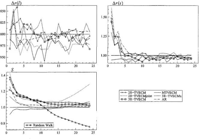
Figure 2 presents the ratios of the MSFEs of the non-linear mo deIs to the VECM, for each of the three variables, セイHャIL@ セイHXI@ and S, for forecast horizons of h
=
1 to 24. The VECM MSFE forms the numerator of the ratio, so values in excess of 1 indicate an improved performance relative to the VECM. It is apparent that allowing for non-linearity contributes relatively little to the ability to forecast セイ@ (l), with gains generalIy less than 5%. The ADM test results in Table 4 indicate that there are no significant differences in the forecast accuracy of the mo deIs at one-step ahead. At a horizon of four-steps the 2R-TVECM is significantly more accurate than the VECM and other non-linear models.The improvement in accuracy of forecasts of セイ@ (8) from allowing for non-linearity is much more marked. Models 2R-TVECM, 2R-TVECMjoint and 3R-TVECM have MSFEs around 50% lower at a horizon of one, and 3R-TVECM is 10% more accurate at four-steps ahead. At one-step ahead, alI non-linear models forecast better than the VECM, except for the MTVECM. At four-steps ahead, the 2R-TVECM and the 3R-TVECM forecast significantly better than the other models. In contrast, at h = 8, non-linear mo deis produce forecasts equivalent to the linear one. These results are in tune with the Pfann et aI. (1996) finding of non-linearity in the short-term interest rate, and also the single-equation equilibrium-correction models for the short-term rate (Anderson, 1997 and van Dijk and Franses, 2000).
The MSFE ratios for the spread indicate smalIer gains than for セイ@ (8), but gains that persist as the horizon lengthens. The gains to non-linearity on MSFE are of 15% to 35% at one-step, and continue (albeit at a lower leveI) for 2R-TVECM and 3R-TVECM. At one-step ahead the 2R-TVECM, the 2R-TVECMjoint and the 3R-TVECM are statistically more accurate than the other models. Even at eight-steps ahead, the rankings on forecast encompassing tests favour the 2R-TVECM and the 3R-TVECM (Table 4). At horizons in excess of 18 months the 2R-TVECMjoint records large gains in accuracy. The reasons are probably due to the 'free' estimation of () (constrained to be 1 in most models) but why this should matter is unclear.
The 2R-TVECM forecasts welI despite the fact that negative spreads do not occur over the forecast period, and that it is during these times that it differs from the VECM model and incorporates a significant 'leveIs effect'. But notice that the VECM and 2R-TVECM suggest quite different dynamic responses (as summarized in the dynamic multipliers reported in table 3). The failure of the VECM to appropriately model behaviour when the spread is negative affects the dynamic responses of the VECM, and its performance is inferior even at more commonly observed values of the spread.
Accuracy as assessed by the GFESM is recorded in Figure 3. 2R-TVECMjoint has the best performance at alI horizons, folIowed by mo deIs 2R-TVECM, 3R-TVECM and 3R-TVECMu ,
confirming the superiority of non-linear models.
6.1 Forecast evaluation conditional upon a regime
The recent literature suggests that non-linear models often record increased gains over linear comparators in some states of nature, but not others (see, for example, Tiao and Tsay, 1994; Clements and Smith, 1997; Clements and Smith, 1999). Comparing mo deIs on MSFE over the whole forecast period, as we have done, is likely to under-estimate the gains that accrue conditional on being in a specific regime.
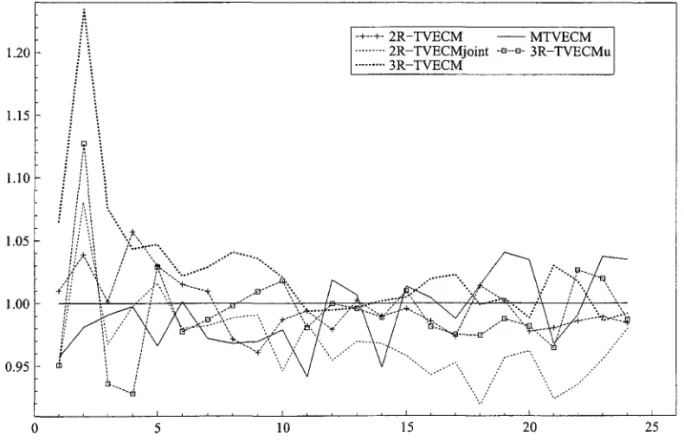
The form of the estimated non-linear mo deis suggests that responses to the equilibrium correction term differ markedly to those implied by the VECM at low (i.e., negative) and high (in excess of 2i) values of the spread, so that we would like to consider forecasts of fl.r (s) and S when the value of the spread at the forecast origin is negative, and forecasts of fl.r (l) when the value of the spread exceeds 2.7. For the majority of the data points the spread is between these two extremes, so the VECM, whose parameter estimates are effectively an average of the regime-specific values, is characterized by very modest mean reversion, and its forecasts are not too dissimilar to those of the non-linear models. However, the spread is never negative over the forecast period. Alternatively, we could consider only those forecasts made when the models' lower regimes were operative, but even this event seldom happened over the forecast periods. Instead, we report results of a forecast evaluation exercise conditioned on St-l
<
O on the simulated data described in section 6.2.For large values of the spread, such as those considered in this evaluation exercise, the 3-regime TVECMs suggest the spread exerts significant downward pressure on r (1). Comparing the relative MSFEs for fl.r (1) in Figures 2 and 4, an improved forecast performance for these mo deis is apparent.
6.2 A simulation exerci se
recurrent recessions. Similarly, the absence of inverted yield curves during the later period might question the relevance of results based on mo deIs which generate such observations.
We generate data from the best 2 and 3-regime models, the 2R-TVECM and the 3R-TVECM, using pseudo random numbers transformed to have the appropriate covariance matrix, and the estimated (full-sample) values of the models' parameters. The number of observations is similar to that in the empirical exercise, and the last 24 observations are kept back for forecasting. These mo deIs and the VECM are then estimated, and used to generate forecasts. Our results are based on Monte Carlo estimates of the MSFEs from 2000 replications.
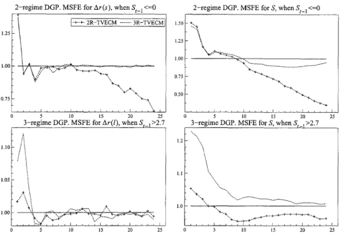
We present the simulation results conditional on the lower regime of negative spreads in the two upper panels of Figure 5. This event characterized around 10% of the simulations, and resulted in gains of around 40 to 50% in predicting f::!.r (8) and S l-step ahead, highlighting
the very different behaviour between the VECM and non-linear models in these circumstances. Notice also that the 2 and 3 regime models behave very similarly because they have the same threshold value for the lower regime. The lower panels in Figure 5 present the MSFE ratios for data generated by the non-linear models, when we consider only those forecasts made (on the roughly 20% of occasions) when the spread exceeded 2.7. The superior performance of the 3-regime model highlights the relevance of allowing for the third regime, at least in the simulation study.
6.3 Comparing with univariate autoregressive models
The choice of the VECM as the linear mo deI comparator may exaggerate the importance of 'non-linearity' from a forecasting perspective if univariate linear autoregressive models are superior to the VECM. So we also generate forecasts from AR mo deIs of f::!.r(8), f::!.r(l), and an AR and a random walk model of the spread. The results in terms of MSFEs are plotted in Figure 2 and show that the linear model forecasts are competitive for f::!.r (8), f::!.r (I), but that the TVECMs are superior than an AR for predicting the spread. The random walk provides accurate forecasts (relative to the other models) of the spread at short horizons, matching the finding that the spread is highly persistent except at high or low values. But these forecasts deteriorate at longer horizons. So, at short horizons cointegration does not improve forecasts of the spread, but some improvement from non-linear cointegration is apparent at longer horizons.
7 Economic interpretation of the models
There is a large academic literature on the term structure of interest rates. In this section we discuss the key features of our models in the light of the expectations theory of the term structure. According to Campbell (1995, p.137-8), the expectations theory implies that:
When long rates are unusually high relative to short rates, long rates do not decline to restore the usual yield curve, as one might suppose. Instead long rates tend to rise; the yield spread falls only because short rates rise even faster.
be lower than current, a pattern reflected in the models. As noted, the VECM suggests very little response of r (s) and r (l) to spreads. From Figure 1 it is apparent that the spread flattens and becomes negative before the economy goes into into recession, so that spreads between long-and short-term interest rates act as usefulleading indicators of recessions (see, e.g., Hamilton and Kim, 2000).
However, for large positive spreads, our mo deis do not exhibit the positive correlation between long rates and the spread predicted by the theory (see the quotation from Camp-belI) , whereby long rates increase, though less quickly than short rates, in response to the long-rate being too high. But see also the evidence against this in Table 2 of CampbelI, p. 139. One strand of argument is that long rates over-react to monetary authority policies aimed at preventing the economy overheating, so that in subsequent periods the disequilibria between the expected values of the short-term rate and the actual long-term rate leads to decreasing long rates, establishing a negative correlation between the spread and long rates5 .
8
Concl usions
Using a variety of different mo deis and tests for non-linear cointegration, we find strong evidence of non-linearities in the response of interest rates to the spread. An evaluation of the forecasting performance of a number of systems mo deis of US short- and long-term interest rates leads us to conclude that non-linearities, including asymmetries in the adjustment to equilibrium, can result in more accurate short horizon forecasts, especially of the spread (i.e., the difference between long and short rates). However, the gains are not alI that large. That non-linearities do not necessarily result in sizable gains is in line with much of the literature. The form of the non-linearity that we identify suggests that linear models will perform relatively welI except when either the yield curve is inverted, or spreads are very high, which are not the norm.
As an advance on much of the previous literature in this area, we apply and adapt the testing and specification techniques to a systems analysis of long- and short-term rates, rather than performing a single-equation analysis of the short-term rate. We confirm that the short-term rate responds to narrowing and negative spreads, but we are also able to show that long-term rates adjust when the spread is too high. Between these two extremes, the spread does not help predict either rate.
The out-of-sample forecast exercise does not clearly favour the 3 over the 2-regime model, but we have shown that the former is to be preferred in certain states of nature, viz. when the spread is high. The non-linear mo deis imply different short-term dynamics depending on whether the yield curve is normal or inverted. Even though the latter has not been observed in recent times, a failure to discriminate between the two historical regimes will bias the coeflicient estimates and may contribute to inferior forecasts. Comparing the forecasts of the non-linear mo deis with univariate models indicates that linear autoregressions are able to produce compet-itive forecasts. However, when forecasts for the spread are evaluated, the gains of non-linearity and cointegration are stronger.
A worthwhile focus for future research in this area would be the possibility of a structural break in the way monetary policy was conducted after 1984, and how this might impact on the
non-linearity in the system. One starting point would be a model in the spirit of Lundbergh et aI. (2000) that allows (possibly smooth) structural breaks in the non-linearity.
References
Anderson, H. M. (1997). Transaction costs and non-linear adjustment towards equilibrium in the US Treasury bill market, Oxford Bulletin of Economics and Statistics 59: 465-484. Anderson, H. M. and Vahid, F. (2000). Predicting the probability of a recession with nonlinear
autoregressive leading indicator models, Monash University, Department of Econometrics and Business Statistics Working Pape r 3/2000.
Bai, J. (1997). Estimating multiple breaks one at a time, Econometric Theory 13: 315-352. Balke, N. S. and Fomby, T. B. (1997). Threshold cointegration, International Economic Review
38: 627-645.
Campbell, J. Y. (1995). Some lessons from the yield curve, Journal of Economic Perspectives
9: 129-152.
Chong, Y. Y. and Hendry, D. F. (1986). Econometric evaluation of linear macro-economic models, Review of Economic Studies 53: 671-690. Reprinted in Granger, C. W. J. (ed.)
(1990), Modelling Economic Series. Oxford: Clarendon Press.
Christoffersen, P. F. and Diebold, F. X. (1998). Cointegration and long-horizon forecasting,
Journal of Business and Economic Statistics 16: 450-458.
Clark, T. E. (1999). Finite-sample properties of tests for equal forecast accuracy, Journal of Forecasting 18: 489-504.
Clark, T. E. and McCraken, M. W. (2000). Tests of equal forecast accuracy and encompassing for nested models, Federal Reserve of Kansas City Working Paper (revised version) 99-11.
Clements, M. P. and Hendry, D. F. (1993). On the limitations of comparing mean squared forecast errors, Journal of Forecasting 12: 617-637. With discussion. Reprinted in T. C. Mills (ed.) Economic Forecasting. The International Library of CriticaI Writings in Economics, Edward EIgar.
Clements, M. P. and Hendry, D. F. (1995). Forecasting in cointegrated systems, Journal of Applied Econometrics 10: 127-146.
Clements, M. P. and Krolzig, H.-M. (1998). A comparison of the forecast performance of Markov-switching and threshold autoregressive models of US GNP, Econometric Journal
1: C47-C75.
Clements, M. P. and Smith, J. (1997). The performance of alternative forecasting methods for SETAR models, International Journal of Forecasting 13: 463-475.
Clements, M. P. and Smith, J. (1999). A Monte Carlo study of forecasting performance of empirical SETAR models, Journal of AppIied Econometrics 14: 123-41.
Dwyer, G. P., Locke, P. and Yu, W. (1996). Index arbritage and nonlinear dynamics between the SP500 futures and cash, Review of FinanciaI Studies 9: 301-332.
Enders, W. and Granger, C. W. J. (1998). Unit-root tests and asymmetric adjustment with an example using the term structure of interest rates, Journal of Business and Economics Statistics 16: 304-31l.
Enders, W. and Siklos, P. L. (2001). Cointegration and threshold adjustment, Journal of Business and Economic Statistics 19: 166-176.
Estrella, A. and Mishkin, F. S. (1998). Predicting US recessions: FinanciaI variables as leading indicators, Review of Economics and Statistics LXXX: 45-61.
Granger, C. W. J. and Teúisvirta, T. (1993). Modelling Nonlinear Economic Relationships,
Oxford University Press, Oxford.
Gray, S. F. (1996). Modeling the conditional distribution of interest rates as a regime-switching process, Journal of Financial Economics 42: 27-62.
Hall, A. D., Anderson, H. M. and Granger, C. W. J. (1992). A cointegration analysis ofTreasury bill yields, Review of Economics and Statistics LXXIV: 116-26.
Hamilton, J. D. and Kim, D. H. (2000). A re-examination of the predictability of economic activity using the yield spread, NBER W orking Papers 7954.
Hansen, B. E. (1996). Inference when a nuisance parameter is not identified under the null hypothesis, Econometrica 64: 413-430.
Hansen, B. E. (2000). Testing for linearity, in D. A. R George, L. Oxley and S. Potter (eds) ,
Surveys in Economic Dynamics, Blackwell, Oxford, pp. 47-72.
Hansen, B. E. and Seo, B. (2000). Testing for threshold cointegration, University of Wisconsin (mimeo) .
Hardouvelis, G. A. (1994). The term structure spread and future changes in long and short rates in the G7 countries, Journal of Monetary Economics 33: 255-283.
Harvey, D. L, Leybourne, S. J. and Newbold, P. (1997). Testing the equality ofprediction mean squared errors, International Journal of Forecasting 13: 281-291.
Harvey, D. L, Leybourne, S. J. and Newbold, P. (1998). Tests for forecasting encompassing,
Journal of Business and Economic Statistics 16: 254-259.
Johansen, S. (1988). Statistical analysis of cointegration vectors, Journal of Economics, Dy-namics and Contral 12: 231-254. Reprinted in R.F. Engle and C.W.J. Granger (eds) , Long-Run Economic Relationships, Oxford: Oxford University Press, 1991, 131-52. Krager, H. and Kugler, P. (1993). Non-linearities in foreign exchange markets: a different
perspective, Journal of International Money and Finance 12: 195-208.
Lundbergh, S. and Terasvirta, T. (2000). Forecasting with smooth transition autoregressive models, SSE/EFI Working Paper in Economics and Finance n. 390.
Lundbergh, S., Terasvirta, T. and van Dijk, D. (2000). Time-varying smooth transition autore-gressive models, SSE/EEI Working Papers in Economics and Finance n. 376.
Mankiw, G. N. and Miron, J. A. (1986). The changing of the term structure of interest rates,
Quaterly Journal of Economics CI: 211-228.
Martens, M., Kofman, P. and Vorst, T. C. F. (1998). A threshold error-correction model for intraday futures and index returns, Journal of Applied Econometrics 13: 245-263. McConnell, M. M. and Perez-Quiros, G. (2000). Output fiuctuations in the United States:
What has changed since early 1980s?, American Economic Review 90: 1464-76.
Montgomery, A. 1., Zarnowitz, V., Tsay, R S. and Tiao, G. C. (1998). Forecasting the US unemployment rate, Journal of American Statistical Association 93: 478-493.
Newbold, P. and Harvey, D. L (2001). Forecasting combination and encompassing, Mimeo,
School of Economics, University of Nottingham. Forthcoming in M. P. Clements and D. F. Hendry (eds), A Companion to Economic Forecasting, (2001), Blackwells.
Pagan, A. R, Hall, A. D. and Martin, V. (1996). Modelling the term structure, in G. S. Maddala and C. R Rao (eds) , Statistical Methods in Finance. Handbook of Statistics
14,
North-Holland, Amsterdam, pp. 91-118.
implications for the term structure, Journal of Econometrics 74: 149-176.
Ramsey, J. B. (1996). If nonlinear models cannot forecast, what use are they?, Studies in Nonlinear Dynamics and Econometrics 1: 65-86.
Roberds, W., Runkle, D. and Whiteman, C. H. (1996). A daily view of yield spreads and short-term interest rate movements, Journal of Money, Credit and Banking 28: 34-53. Rothman, P. (1998). Forecasting asymmetric unemployment rates, Review of Economics and
Statistics 53: 164-168.
Rudebusch, G. D. (1995). Federal reserve interest rate targetting, rational expectations, and the term structure, Journal of Monetary Economics 35: 245-174.
Stock, J. H. and Watson, M. W. (1999). A comparison of linear and nonlinear univariate models for forecasting macroeconomic time series, in R. F. Engle and H. White (eds),
Cointegration, Causality and Forecasting: A Festschrift in Honour of Clive Granger, Ox-ford University Press, OxOx-ford, pp. 1-44.
Tiao, G. C. and Tsay, R. S. (1994). Some advances in non-linear and adaptative modelling in time series, Journal of Forecasting 13: 109-131.
Tong, H. (1995). Non-linear Time Series. A Dynamical System Approach, Clarendon Press, Oxford. First published 1990.
Tsay, R. S. (1989). Testing and modeling threshold autoregressive processes, Journal of the American Statistical Association 84: 231-240.
Tsay, R. S. (1998). Testing and modeling multivariate threshold models, Journal of the Amer-ican Statistical Association 93: 1188-1202.
Tzavalis, E. and Wickens, M. (1998). A re-examination of the rational expectations hypo-thesis of the term structure: Reconciling the evidence from long-run and short-run tests,
lnternational Journal of Finance and Economics 3: 229-239.
van Dijk, D. (1999). Smooth Transition Models: Extensions and Outlier Robust lnference, PhD thesis, Tinbergen Institute.
van Dijk, D. and Franses, P. H. (2000). Nonlinear error-correction models for interest rates in the Netherlands, in W. A. Barnett, D. F. Hendry, S. Hylleberg, T. Terasvirta, D. Tjostheim and A. Wurtz (eds) , Nonlinear Econometric Modelling in Time Series: Proceedings of the Eleventh International Symposium in Economic Theory, Cambridge University Press, Cambridge.
West, K. D. (1996). Asymptotic inference about predictive ability, Econometrica 64: 1067-1084. West, K. D. and McCracken, M. W. (1998). Regression-based tests of predictive ability,
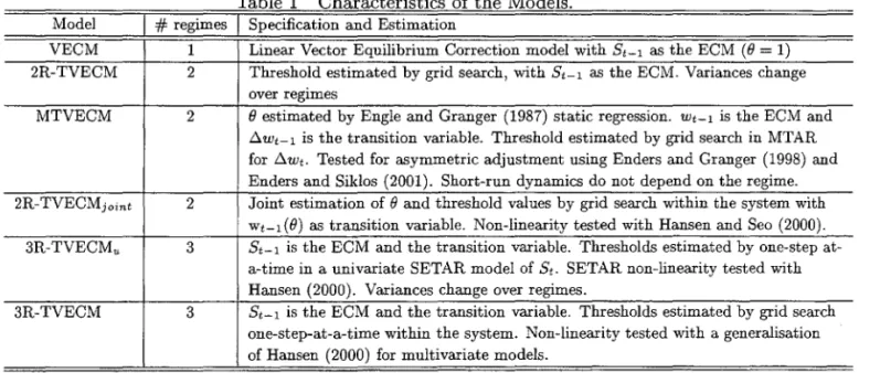
TabIe 1 Characteristics of the Models.
Model # regimes
I
Specification and EstimationVECM 1 Linear Vector Equilibrium Correction model with St-1 as the ECM (f) = 1) 2R-TVECM 2 Threshold estimated by grid search, with St-1 as the ECM. Variances change
over regimes
MTVECM 2 f) estimated by Engle and Granger (1987) static regression. Wt-1 is the ECM and
セwエMQ@ is the transition variable. Threshold estimated by grid search in MTAR
for セwエN@ Tested for asymmetric adjustment using Enders and Granger (1998) and Enders and Siklos (2001). Short-run dynamics do not depend on the regime. 2R-TVECMjoint 2 Joint estimation of f) and threshold values by grid search within the system with
Wt-l (f)) as transition variable. Non-linearity tested with Hansen and Seo (2000). 3R-TVECM" 3 St-1 is the ECM and the transition variable. Thresholds estimated by one-step
at-a-time in a univariate SETAR model of St. SETAR non-linearity tested with
Hansen (2000). Variances change over regimes.
3R-TVECM 3 St-1 is the ECM and the transition variable. Thresholds estimated by grid search one-step-at-a-time within the system. Non-linearity tested with a generalisation of Hansen (2000) for multivariate models.
15
10
5
1960196219641966196819701972 1974 19761978 1980198219841986198819901992 1994199619982000
UNPセセMMMMMMMMMMMMMNNMMMセセMMMMMMMNNMNMGMMMMMMMMMMMMNイMMMMMMMMMMMMMセ@
2.5
0.0
-2.5
1960196219641966196819701972 197419761978 19801982198419861988199019921994199619982000
Table 2 Testing for unit roots and non-linearity
Tests 1960:1-1989:12 1960:1-1998:4
r(s), -1.699 r(s), -1.890
Augmented Dickey-Fuller r(l), -1.572 r(l), -1.736
1 .6.r(s) , -8.65h .6.r(s), -9.633*
Unit Roots
.6.r(l) , -7.870* .6.r(l) , -7.109*
S, -2.497 S - 2.795
2 Phillips-Perron Unit Root S, -3.716* S - 3.899*
3 J ohansen cointegration (trace) 16.88* 18.6*
Enders and Siklos <P, 9.84* <P,1O.9h
4 Asymmetric Cointegration t - max, -3.96* t - max, -4.26*
(TAR) Pl
=
P2, 2.84[0.09] Pl=
P2, 4.42* [0.04]Enders and Siklos <P, 8.39* <P, 8.63*
5 Asymmetric Cointegration t - max, -3.20* t - max, -3.07*
(M-TAR) Pl
=
P2, 0.11[0.74] Pl=
P2, 0.01[0.91]6 Hansen and Seo 25.183* [0.00] 34.527* [0.00]
Threshold cointegration
7 Threshold Cointegration 45.17* [0.002] 52.43* [0.00]
linear vs. two-regime
8 Threshold Cointegration 11.09 [0.17] 10.08 [0.14]
two-regime vs. three-regime
9 System non-linearity (eq. 7)
linear vs. two-regime 149.71* [0.01] 182.88* [0.01]
10 System non-linearity 62.24* [0.02] 71.29* [0.03]
two-regime vs. three-regime
d
=
1, 116.98*[0.00] d=
1, 110.54*[0.00]11 Tsay d
=
2, 68.83*[0.00] d=
2, 63.94*[0.00]System non-linearity d
=
3, 105.23*[0.00] d=
3,130.13*[0.00]d
=
4, 87.39*[0.00] d=
4, 195.43*[0.00] * null hypothesis rejected at least at 5%TabIe 3 ResuIts of the estimation of the mo deIs
M T Lower regime Middle regime Upper regime
Mult. St-l, TL Mult. St-l, TM Mult. St-l, TU fl,r2
.6.r(s) Wt-l .6. r ( s) Wt-l .6. r ( s) Wt-l
(B)
eq .6.r(l) OiL .6.r(l) OiM .6.r(l) OiuVEqCM 60-89 .6. r ( l) 0.009 -0.025
.6.r(s) 0.440 0.058* 60-98 .6.r(l) -0.007 -0.026*
.6.r(s) 0.411 0.046*
2R- 60-89 .6.r(l) -0.132 0.037 61 0.077 -0.022 295 0.06
TVEqCM .6.r(s) 1.217 0.608* 0.077 0.036
60-98 .6.r(l) -0.132 0.037 61 0.059 -0.020 395 0.06
.6. r ( s) 1.217 0.608* 0.122 0.027
M- 60-89 .6.r(l) 0.010 -0.011 -0.037 0.39
TVEqCM .6.r(s) 0.440 0.044 0.127* (1.14)
60-98 .6.r(l) -0.003 -0.009 -0.038 0.39
.6.r( s) 0.418 0.033* 0.112* (1.16)
2R- 60-89 .6.r(l) 0.142 0.006 52 -0.006 -0.010 303 -4.35
TVEqCM .6. r ( s) 1.883 0.185* 0.329 0.004 (1.54)
joint 60-98 .6.r(l) 0.199 0.008 83 -0.070 -0.014 372 -2.5
.6.r(s) 1.609 0.203* 0.282 0.001 (1.40)
3R- 60-89 .6.r(l) -0.132 0.037 61 0.099 -0.006 254 -0.071 -0.407* 41 0.06,
TVEqCM .6.r( s) 1.217 0.608* -0.085 0.004 0.217 0.187 2.74
u 69-98 .6.r(l) -0.132 0.037 61 0.023 -0.002 344 0.171 -0.240 51 0.06,
.6.r(s) 1.217 0.608* 0.105 0.015 0.083 0.338 2.86
3R- 60-89 .6.r(l) -0.132 0.037 61 0.100 -0.021 244 -0.074 -0.426* 51 0.06,
TVEqCM .6. r ( s) 1.217 0.608* -0.087 -0.019 0.183 0.016 2.62
60-98 .6.r(l) -0.132 0.037 61 0.075 -0.017 321 -0.031 -0.309* 74 0.06,
.6.r(s) 1.217 0.608* -0.013 0.003 0.286 0.042 2.71
* statistically significant at 5%.
Notes: The models are summarised in Table 1; The long-run multipliers (Mult.) are calculated for each equation treating .6.r(s) or .6.r(l) as exogenous. The Oii for i = L ,M, U (lower, middle and upper regime) are the
coefficients of the spread variable (St-l) or the cointegrated relationship (Wt-l
=
rt-l (I) - Brt-l (s)). Ti refers to the number of observations in each regime.Table 4 Rank of tests of forecast accuracy and forecast encompassing.
Augmented Diebold and Mariano Forecast Accuracy test - Ranks
.6.r(l) .6.r(s) S
h=l
I
h=2I
h=4I
h=8 h=lI
h=2I
h=4I
h=8 h=lI
h=2I
h=4-r
h=8VECM 1 2 2 3 4 3 3 1 3 3 3 2
2R-TVECM 1 1 1 2 2 2 1 1 2 2 1 1
MTVECM 1 2 3 3 5 4 3 2 4 4 3 2
2R-TVECMjoint 1 2 3 3 1 1 3 2 1 1 3 2
3R-TVECMu 1 2 3 1 3 2 3 2 4 4 3 2
3R-TVECM 1 2 2 2 2 2 2 1 2 1 2 2
Forecast Encompassing test - Ranks
.6.r(l) .6.r(s) S
h=l
I
h=2I
h=4I
h=8 h=lI
h=2I
h=4I
h=8 h=lI
h=2I
h=4I
h=8VECM 2 4 3 1 4 3 3 1 3 4 3 3
2R-TVECM 1 3 1 1 3 2 2 1 2 1 2 2
MTVECM 2 5 3 3 5 4 4 3 5 5 3 3
2R-TVECMjoint 1 1 3 3 2 1 4 3 1 1 2 3
3R-TVECMu 3 2 3 1 3 2 4 2 4 3 3 3
3R-TVECM 2 3 2 2 1 1 1 2 1 2 1 1
Notes:
I'1rl /j.r s 1.050
1.50 1.025
1.000
0.975
0.950
O 25 25
S
.,0'
-".,- +-+-2R-TVECM - MTVECM
--.---- 2R-TVECMjoint ---·3R-TVECMu
-B--E>. 3R-TVECM - - AR
. MセMNNZNZG]MM
0.8
I ... Random Walk 1
O 10 20 25
Figure 2 Ratio of MSFEs for VECM against non-linear models, for .6.r(l), .6.r(s) and S.
1.6
1.5
1.4
1.3
1.2
1.1
1.0
O 5 10 15
1
-+--+-2R-TVECM - - MTVECM 11
··---·2R-TVECMjoint -s--s- 3R-TVECMt ·--"-"·3R-TVECM
20 25
1.20
1.15
'?
1.05
1.00 1.10
i
II \
./:,f.'.:.>\\\\" ..
ャNᄋNᄋNGNᄋNᄋNᄋNセNセNLZZLZNᄋZZZ[ZZZZセZセᄋLLᄋᄋᄋᄋᄋᄋᄋ@
... ···
, \ T
ORNMMZZZセZZZZ@
...
f
0.95
o 5 10
-+--+-2R-TVECM - - MTVECM
···2R-TVECMjoint ." .. ". 3R-TVECMu ···3R-TVECM
-""
15 20 25
Figure 4 Ratio of MSFE for S for l:::.r(l) of VECM to the non-linear models, conditional on
2-regime DOP. MSFE for tl.r(s), when SI_1 <=0 2-regime DOP. MSFE for S, when SI_l <=0
I
I-+-+ 2R-TVECM m m 3R-TVECMI1.25
1.00
V\P
セG@0.75
5 10 15 20 25 5 10 15 20 25
3-regime DOP. MSFE for tl.r(l), when S _ >2.7 3-regime DOP. MSFE for S, when S >2.7
10 15 20 25 10 15 20 25
000307810