Diego Paolo Ferruzzo Correa
SYMMETRIC BIFURCATION ANALYSIS OF SYNCHRONOUS
STATES OF TIME-DELAY OSCILLATORS NETWORKS
Diego Paolo Ferruzzo Correa
SYMMETRIC BIFURCATION ANALYSIS OF SYNCHRONOUS
STATES OF TIME-DELAY OSCILLATORS NETWORKS
Text presented to Escola Politécnica da Uni-versidade de São Paulo as a thesis to obtain a PhD degree in Electrical Engineering.
Specific area: Systems Engineering
Supervisor:
Prof. PhD. José Roberto Castilho Piqueira
Acknowledgments
Resumo
Nos últimos anos, tem havido um crescente interesse em estudar redes de osciladores aco-pladas com retardo de tempo uma vez que estes ocorrem em muitas aplicações da vida real. Em muitos casos, simetria e padrões podem surgir nessas redes; em consequência, uma parte do sistema pode repetir-se, e as propriedades deste subsistema simétrico repre-sentam a dinâmica da rede toda. Nesta tese é feita uma análise de uma rede deN nós de segunda ordem totalmente conectada com atraso de tempo. Este estudo é realizado utili-zando grupos de simetria. É mostrada a existência de múltiplos valores próprios forçados por simetria, bem como a possibilidade de desacoplamento da linearização no equilíbrio, em representações irredutíveis. É também provada a existência de bifurcações de estado estacionário e Hopf em cada representação irredutível. São usados três modelos diferentes para analisar a dinâmica da rede: o modelo de fase completa, o modelo de fase, e o modelo de diferença de fase. É também determinado um conjunto finito de freqüências ω, que pode corresponder a bifurcações de Hopf em cada caso, para valores críticos do atraso. Apesar de restringir a nossa atenção para nós de segunda ordem, os resultados podem ser estendido para redes de ordem superior, desde que o tempo de atraso nas conexões entre nós permanece igual.
Palavras-chave: Simetria. Grupo de Lie. Rede de osciladores. Sistemas com atraso de tempo. Bifurcações. Equações diferencias com atraso.
Abstract
In recent years, there has been increasing interest in studying time-delayed coupled net-works of oscillators since these occur in many real life applications. In many cases sym-metry, patterns can emerge in these networks; as a consequence, a part of the system might repeat itself, and properties of this symmetric subsystem represent the whole dy-namics. In this thesis, an analysis of a second order N-node time-delay fully connected network is made. This study is carried out using symmetry groups. The existence of multiple eigenvalues forced by symmetry is shown, as well as the possibility of uncoupling the linearization at equilibria, into irreducible representations due to the symmetry. The existence of steady-state and Hopf bifurcations in each irreducible representation is also proved. Three different models are used to analyze the network dynamics, namely, the full-phase, the phase, and the phase-difference model. A finite set of frequenciesω is also determined, which might correspond to Hopf bifurcations in each case for critical values of the delay. Although we restrict our attention to second order nodes, the results could be extended to higher order networks provided the time-delay in the connections between nodes remains equal.
Keywords: Symmetry. Lie group. Oscillator network. Time-delay system. Bifurcations.
Delay differential equations.
List of Figures
Figure 3.1 Symmetry-preserving bifurcation curves for the equilibria x∗
1 =φ±,
with K = 1 and 0< µ <2. . . 26 Figure 3.2 Real part of the rightmost root for the characteristic functionPFix(SN)
with K = 2 and x∗
1 =φ+, forµ={0.1, 0.2, 0.4, 0.6, 0.8}. . . 27
Figure 3.3 Real part of the rightmost roots for the characteristic function
PFix(SN) with K = 2 and x∗1 =φ+, forµ= 0.9 using DDE-Biftool. . 27
Figure 3.4 Symmetry-preserving bifurcation curves for the equilibrium x∗
1 =
φ−, withK = 1.05. . . 29
Figure 3.5 Real part of the rightmost root of PFix(SN) for x1∗ = φ−, µ = 0.3,
and K = 1.05, using DDE-Biftool. . . 30 Figure 3.6 Curves showing conditions for the existence of symmetry-breaking
bifurcations with x∗
1 =φ+ and K >1. . . 34
Figure 3.7 Symmetry-preserving bifurcation curves and symmetry-breaking bi-furcation curves for both equilibria x∗
1 =φ± with N = 2 and K = 1. 36
Figure 3.8 Real part of the rightmost root for the function Pj, for N = 2,
K = 1 and µ={0.05, 0.5, 1}. . . 37 Figure 3.9 Symmetry-preserving bifurcation curves and symmetry-breaking
bi-furcation curves forµ+ and forµ− withN = 3 andK = 1, for both
equilibriax∗
1 =φ±. . . 38
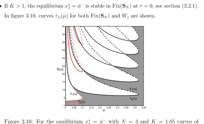
Figure 3.10 For the equilibrium x∗
1 = φ− with N = 3 and K = 1.05 curves of
symmetry-preserving bifurcations and curves of symmetry-breaking bifurcations. . . 39
Figure 4.1 CurvesK+(µ;ωM, n, m)from (4.16) andδ+(µ, K(µ);m)withωM =
1, n = 1 for different values of m. . . 46 Figure 4.2 Curves Ωb with µ= 1,K = 1, and ωM = 1. . . 47
Figure 4.3 Snmaps for curvesΩb(j)related to the characteristic functionPFix(SN);
in all cases, δ(ω(τ∗)) is positive. . . 48
Figure 4.4 Sn maps for different curvesΩb related to the characteristic function Pj; in all cases, δ(ω(τ∗))is positive. . . 51
Figure A.1 PLL block diagram . . . 65
Figure A.2 2-node network . . . 66
Figure A.3 PLL with multiple inputs. . . 67
List of Symbols
C The set of complex numbers
Fix(H) The fixed-point subspace ofH
Im(z) The imaginary part of the complex numberz
X The Banach space of continuous functions from [−τ,0]into RN
N The set of natural numbers
R The set of real numbers
Re(z) The real part of the complex number z
Dm The dihedral group of order 2m
Sm The symmetric group consisting of all permutations onm symbols
Zm The cyclic group of order m
Z The set of integers numbers
Acronyms
DDE Delay Differential Equation
PLL Phase Locked Loop
RFDE Retarded Functional Differential Equation
VCO Voltage-controlled oscillator
Contents
1 Introduction 1
2 Literature review 3
2.1 Delay differential equations . . . 3
2.2 Characterization of spatio-temporal symmetries . . . 5
2.2.1 Symmetry of solutions . . . 7
2.2.2 Relative Equilibria . . . 9
2.3 Method of steps for solution of DDE . . . 9
2.4 Lambert W function . . . 10
2.5 TheSn map . . . 12
3 Full-phase model 15 3.1 SN-symmetry and irreducible representations . . . 16
3.2 Symmetry-preserving bifurcations . . . 21
3.2.1 Roots in the characteristic function PFix(SN) at τ = 0 and asτ → ∞ 22 3.2.2 Conditions for the existence of symmetry-preserving bifurcations . . 22
3.2.3 Curves of symmetry-preserving bifurcations . . . 24
3.3 Symmetry-breaking bifurcations . . . 30
3.3.1 Roots in the characteristic function Pj at τ = 0 and as τ → ∞ . . . 30
3.3.2 Conditions for the existence of symmetry-breaking bifurcations . . . 31
3.3.3 Curves of symmetry-breaking bifurcations . . . 36
3.4 Equivariant Hopf bifurcations forN = 2,3 . . . 40
4 Phase model 41 4.1 Symmetry-preserving bifurcations . . . 43
4.1.1 Symmetry-preserving bifurcations from equilibria . . . 45
4.2 Symmetry-breaking bifurcations . . . 48
4.2.1 Symmetry-breaking bifurcations of relative equilibria . . . 49
4.2.2 Symmetry-breaking bifurcations from equilibria . . . 50
4.2.3 Curves of symmetry-breaking bifurcations . . . 51
5 Phase-difference model 53 6 Conclusions and Future work 57 6.1 Conclusions . . . 57
6.2 Future Work . . . 58
Appendix A The PLL network model 65
Chapter 1
Introduction
Networks of oscillators have been a topic of study for decades since their models can rep-resent several complex dynamics, and results can be applicable in many different areas, such as biology, neurology, economics, and astronomy (Győri and Ladas, 1991; Li, Yang, Wen, and Wang, 2014; Martins and Monteiro, 2013; Piqueira, 2011; Smith, 2011; Strogatz, 2001). Nevertheless, in recent years, much attention has been focused in some emergent behaviors which cannot be explained considering the dynamic of individual nodes isol-atedly; those behaviors seem to originate in the network structure itself. In that sense, great effort has been applied to understand the influence that changes in the parameter space associated to the network structure can have over the global dynamics. In this work, we study the influence of a non-ideal connection between nodes in a fully-connected
N-oscillator network, represented by a constant time-delay. It has already been shown that this delay is responsible for instability, chaotic behavior and bifurcations in oscillat-ors networks; The global exponential stability is explored in Li et al. (2014); Yuan and Zhao (2012), the nonlinear case is studied in Vuellings, Schoell, and Lindner (2014), the linear coupling case is studied in Giannakopoulos and Zapp (2001), and the linear stabil-ity for nonlinear coupling is addressed in Olien and Belair (1997); Song and Xu (2013). In our approach, we shall analyze the influence of this time-delay in the emergence of bifurcations from equilibria.
The structure of this thesis is as follows: In chapter two, a literature review is made covering the main concepts and tools used along the thesis, with special emphasis in some useful results related to DDEs; most of the proofs are omitted since we focus on the results and applicability of the concepts. In chapter three, the Full-phase model is introduced
Chapter 2
Literature review
One of the main issues when dealing with DDEs is the number of roots emerging in the characteristic equation, whilst in ODEs this number is always finite and matches the order of the equation, in DDEs the number of roots is infinite. However, most of the well know results concerning stability and linearization in ODEs can be extended, no without some work, to DDEs. In what follows some important results about retarded differential equations and symmetry, will be presented.
2.1
Delay differential equations
Delay differential equations (DDE) which are the class of differential equations that emerge when time-delay is considered in models of oscillators networks are a special case of the so-called Functional differential equations (FDE). In this section, we will review some basics related to FDE applied to DDE following Gilsinn (2009); Gorecki, Fuksa, Grabowski, and Kotytowski (1989); Hale (1977); Krawcewicz and Wu (1999); Kuang (1993); Michiels and Niculescu (2007); Smith (2011); Wu (1998). Let τ ≥0 be a given constant,N a positive
integer and X := C([−τ,0],RN) the Banach space of continuous functions from [−τ, 0] intoRN equipped with the usual supremum norm.
kϕk= sup
−τ≤θ≤0|
ϕ(θ)|, ϕ∈ X.
Ifx : [−τ, A] →RN is a continuous function with A >0 and if t ∈[0, A], then xt∈ X is defined by
xt(θ) =x(t+θ), θ ∈[−τ,0].
4 CHAPTER 2. LITERATURE REVIEW Let the autonomous nonlinear DDE
˙
x(t) =f(x(t), x(t−τ), η), (2.1)
where η ∈ Rp is a vector of parameters, x(t) ∈ RN, and x(t − τ) ∈ X, such that
f(x∗, x∗, η)=0, for some equilibrium x∗
∈ RN, clearly f : RN × X × Rp → RN. We can linearize (2.1) around its equilibrium and obtain
˙
x(t, η) =U(η)x(t) +V(η)x(t−τ) +F(x(t), x(t−τ), η) (2.2)
where U(η) = ∂x∂(t)f(x∗, x∗, η), V(η) = ∂ ∂x(t−τ)f(x
∗, x∗, η), and F(x(t), x(t
−τ), η) is a nonlinear term. For the linear part of (2.2) the map T :X →RN is a family of solution operators
(T(t)φ))(θ) = (xt(φ))(θ) =x(t+θ), φ∈ X,
xt(φ)is the flow in X at time t. The family of operators T(t) satisfies:
• T(t) is bounded and linear for t≥0
• T(0)φ=φ or T(0) =I
• lim
t→t0k
T(t)φ−T(t0)φk= 0,
wherek · kC is aX norm. This family of operators is called a semigroup. We can associate
to the semigroup T(t)an infinitesimal generator:
Aφ= lim
t→t+ 0
1
t[T(t)φ−φ],
defined as:
(A(η)φ) =
dφ
dθ , −τ ≤θ <0
U(η)φ(0) +V(η)φ(−τ) , θ= 0,
(2.3)
then T(t)φ satisfies
d
dtT(t)φ=A(η)T(t)φ,
where d
dtT(t)φ = limh→0
1
h[T(t−h)φ−T(t)φ]. Then the operator form for equation (2.2) is d
2.2. CHARACTERIZATION OF SPATIO-TEMPORAL SYMMETRIES 5
A(η) and G(·, η)map into X, and
(G(φ;η))(η) =
0 , −τ ≤θ ≤0
F(φ(0), φ(−τ), η) , θ = 0.
The characteristic equation for the linear part of (2.2) is obtained by looking for nontrivial solution of the form eλtc wherecis a constant vector. Then the linear part of (2.2) has a
nontrivial solutioneλtcif and only if
det(△(λ, τ, η)) = 0, (2.4)
where
△(λ, τ, η) :=λId−L(η, τ) (2.5)
is thecharacteristic matrix and the linear operator
L(η, τ) :=U(η) +V(η)e−λτ, (2.6) maps X into RN. We define the transcendental characteristic function associated to the linear part of (2.2) as
P(λ, τ, η) :=det(△(λ, τ, η)) = 0. (2.7)
The spectrumσ(A(η)) of A(η) consists of eigenvalues which are solutions of (2.4).
2.2
Characterization of spatio-temporal symmetries
The oscillator networks studied here present symmetries, which are specified in terms of a group of transformations of the variables in their models that in some sense preserve the structure of the equations and their solutions (Collera, 2012; Dias and Rodrigues, 2009; Golubitsky and Stewart, 2002; Golubitsky, Stewart, and Schaeffer, 1988). We shall consider the main following groups:
• Dm the dihedral group of order2m (rotation and reflections in the plane).
• Zm the cyclic group of order m (rotations only).
6 CHAPTER 2. LITERATURE REVIEW • R the translational group, which we take to act as
x1 ... xn → x1 ... xn + C ... C
, C ∈R.
Since f : X → RN in equation (2.1) is a continuously differentiable function with sym-metry, then, there exists a compact Lie group Γ as well as an orthogonal representation
ρ : Γ → GL(RN). For details, see Collera (2012); Ruan, Krawcewicz, Farzamirad, and Balanov (2006).
We say that system (2.1) is equivariant with respect to the action of Γ on RN, or Γ-equivariant, if:
f(ρ(γ)ϕ) =ρ(γ)f(ϕ), ϕ ∈ X, γ ∈Γ,
where ρ(γ)ϕ∈ C[−τ,0]is defined by
(ρ(γ)ϕ)(θ) = ρ(γ)ϕ(θ), θ ∈[−τ,0].
The subset H of Γ that fixes a point ϕ ∈ X forms a subgroup of Γ. This subgroup is called the isotropy group of ϕ, and is denoted by Hϕ ={g ∈Γ | gϕ=ϕ}.
Definition 2.1 (The fixed-point subspace). Let H be a subgroup of Γ. The fixed-point subspace of H is given by
Fix(H) ={ϕ ∈ X | hϕ=ϕ, ∀h∈H}.
Iff isΓ-equivariant and H is a subgroup ofΓ, then f(Fix(H))⊆Fix(H). This means that we can find an equilibrium solution with isotropy subgroup H by restricting the system in (2.1) to a subspace Fix(H). In addition, the operator△(λ, τ, η)defined in (2.5) is also Γ-equivariant.
In general, a spaceV is calledΓ-invariant ifgV ⊆V, for allg ∈Γ; as a consequence, it is always possible decompose the space intoΓ-invariants subspaces of smaller dimension. The smallest blocks for such decomposition are said to be irreducible. A space V is Γ-irreducible if the only Γ-invariant subspaces of V are {0} and V itself. Let W ⊂V be a Γ-invariant subspace. Then there exists aΓ-invariant complementary subspace W⊥ such
that
2.2. CHARACTERIZATION OF SPATIO-TEMPORAL SYMMETRIES 7 LetΓ be a compact Lie group acting onV. Then there exists Γ-irreducible subspaces
V1, . . . , Vs of V such that
V =V1⊕ · · · ⊕Vs,
this decomposition is not unique and is called Complete Reducibility. Up toΓ-isomorphism there are a finite number of distinctΓ-irreducible subspaces ofV, calledU1, . . . , Ut. Define
Wk to be the sum of all Γ-irreducible subspaces W of V such that W isΓ-isomorphic to
Uk. Then
V =W1⊕ · · · ⊕Wt.
This generates a unique decomposition ofV into the so-called isotypic components. A representation of a group Γ on a vector spaceV is said to be absolutely irreducible if the only linear mapping onV that commutes withΓare scalar multiples of the identity, that is{cI | c∈R} is the only mapping that commutes with Γ.
Therefore, for the dynamics 2.1 of a N-oscillator fully connected network with sym-metry, for all N, there is an N-dimensional representation of the symmetric group of order N, called the permutation representation, which consists of permuting N coordin-ates. This has the trivial subrepresentation consisting of vectors whose coordinates are all equal. The orthogonal complement consists of those vectors whose coordinates sum is zero, and whenN ≥2, the representation on this subspace is anN−1-dimensional irredu-cible representation, called the standard representation. In other words,RN decomposes as
RN = Fix(H)⊕U, and U = Fix(H)⊥ ∼
=RN−1 is SN-invariant and irreducible.
2.2.1
Symmetry of solutions
Assume (2.1) has a periodic solution x(t). There are two types of symmetry that make the solution invariant. The first one is the group of spatial symmetries
8 CHAPTER 2. LITERATURE REVIEW which is the isotropy group of each point on the solution. The second is the group of spatio-temporal symmetries
H ={γ ∈Γ, γx(t) =x(t+t0(γ)), for all t}
where t0(γ)≥ 0. Clearly, spatial symmetries are those spatio-temporal symmetries γ for
which t0 = 0.
Lemma 2.1. Group K is a normal subgroup of H (Collera, 2012).
Each element γ ∈ H corresponds to a time phase-shift t0(γ). If the periodic solution
has period T, thent0(γ)∈R/TZ∼=S1. Then the mapping
t0 :H →S1
is a homomorphism. Moreover, ker(t0) is composed of all γ ∈ H with t0(γ) = 0, that
is, ker(t0) = K. From the first Isomorphism Theorem, given the group homomorphism
t0 :H →S1, we have
Im(t0)∼=H/K,
which means that H/K is isomorphic to a closed subgroup of S1. Since the only closed
subgroups of S1 are Z
m, m≥1, and itself, we have
H/K ∼=S1 or H/K ∼=Zm, m≥1.
When H/K ∼=S1, the periodic solution is called arotating wave, while ifH/K ∼=Zm, the
periodic solution is called a discrete rotating wave (Golubitsky et al., 1988).
Theorem 2.1. LetΓbe a finite group acting on X. There is a T-periodic solution of the Γ-equivariant system in (2.1) with spatial symmetry K and spatio-temporal symmetryH
with
hx(t) = x
t− T m
for some fixed h∈N(K) if and only if
(a) H/K ∼=Zm is cyclic, m≥2, and h∈H projects onto a generator of H/K,
2.3. METHOD OF STEPS FOR SOLUTION OF DDE 9 (c) dim Fix(K) ≥ 2. If dim Fix(K) = 2, then H = N(K) and h acts on Fix(K) by
rotation through±2π m,
(d) H fixes a connected component of Fix(K)\LK, where
LK =
[
γ6=K
Fix(γ)∩Fix(K).
2.2.2
Relative Equilibria
An equilibrium point is a point in the phase space that is invariant under the dynamics:
ϕ ∈ X for which f(ϕ) = 0 or equivalent ϕ˙ = 0. We can define relative equilibrium as a group orbit that is invariant under the dynamics.
Definition 2.2(Relative Equilibria). A relative equilibrium is a trajectoryϕ(t)∈ C[−τ,0] such that for eacht∈Rthere is a 1-parameter family of symmetry transformation γt∈Γ for which ϕ(t) = γtϕ(0).
This means the trajectory is contained in a single group orbit. Clearly, if a group orbit is invariant under dynamics, then all the trajectories in it are relative equilibria; conversely, if ϕ(t) is the trajectory through p, then γϕ(t) is the trajectory through γp
and accordingly the entire group orbit is invariant (Fiedler, Sandstede, Scheel, and Wulff, 1996; Montaldi, 2000).
Definition 2.3(Relative periodic orbit). A relative periodic orbit (RPO) of aΓ-equivariant dynamical systemX˙ =F(X) with phase space X is periodic orbit in the space of group orbits X/Γ. If Γ is compact, then a trajectory X(t)lies on an RPO if and only if it is a periodic orbit in a comoving frame, see, e.g., Fiedler et al. (1996).
2.3
Method of steps for solution of time-delay
differen-tial equations
Also called sequential integration method, it is the basic form to solve time-delay differ-ential equations with constant delays. The solution is found for each successive interval, one by one, by solving a simple ODE at each interval. Consider the following nonlinear DDE with unique time-delay:
˙
10 CHAPTER 2. LITERATURE REVIEW
with τ > 0. Suppose f(t, x, y) and ∂
∂xf(t, x, y) are both continuous into R
3, let s ∈ R
and φ : [s−τ, s]→R continuous. We are looking for a solutionx(t) of (2.8) such that
x(t) =φ(t), s−τ ≤t≤s (2.9)
and satisfying (2.8) within interval s≤t ≤s+σ for some σ >0. For s≤t ≤s+τ,x(t) has to satisfy the ODE initial condition problem:
˙
y(t) = f(t, y(t), φ(t−τ)), y(s) = φ(s), s ≤t≤s+τ
since f(t, y, φ(t −τ)) and ∂
∂yf(t, y) are both continuous, thecc solution is guaranteed
within interval s ≤ t ≤ s+τ; then, solution x(t) is defined within interval [s−τ, s+τ] and it is possible to extend such solution to the right by repeating the process. In fact, for s+τ ≤ t ≤ s+ 2τ, solution x(t) of (2.8) and (2.9) have to satisfy the ODE initial condition problem:
˙
y(t) = f(t, y(t), x(t−τ)),
y(s+τ) = x(s+τ), s+τ ≤t≤s+ 2τ
Theorem 2.2. Let f(t, x, y) and ∂
∂xf(t, x, y) continuous into R
3, s ∈ R and let φ :
[s−τ, s]→Rcontinuous. Then, someσ > sexists and a unique initial condition problem solution (2.8)-(2.9) within interval [s−τ, σ].
2.4
Lambert
W
function
Although the number of roots in the characteristic function associated to the linear part in (2.2) is infinite, the stability of the delay equation (2.1) depends on whether there is any root with positive real part or not. Wang (2008) presents a numerical method to compute the rightmost characteristic root for a time-delay linear system using the Lambert W
function; the critical poles closest to the imaginary axis, which determine the stability of the system, correspond to the principal branch (W0) of the Lambert W function. These
2.4. LAMBERT W FUNCTION 11 functionw7→wew, which is the solution of the transcendental equation
wew =z, z ∈C,
solutionW(z)has infinite many branches, Wk(z), k∈Z, the branches are
W0(z) =
∞
X
n=1
(−n)n−1
n! z
n,
Wk(z) = lnk(z)−ln(lnk(z)) +
∞
X
l=0
∞
X
m=1
Clm
(ln(lnk(z)))m
(lnk(z))l+m
,
wherelnk(z) = ln(z) + 2πki indicates the k-th logarithm branch, and the coefficientsClm
can be expressed in asClm =
(−1)l
m!
l+m l+1
. Shinozaki and Mori (2006) demonstrated that
Re[W0(z)] =max
k∈Z Re[Wk(z)].
For the time-delay scalar linear system,
˙
y(t) +ay(t−τ) +by(t) = 0,
wherea, b∈C and y(t)∈R, and τ >0. The characteristic equation
λ+ae−λτ +b = 0,
can be written as
(λ+b)τ e(λ+b)τ =−aτ ebτ,
and in terms of the Lambert W function, we see that
(λ+b)τ =Wk(−aτ ebτ),
and the characteristic roots are
λ= 1
τWk(−aτ e
bτ)
−b,
which can be computed right away. For the characteristic function
P(λ) = λ2+aλ+b+ce−λτ = 0, a, b, c∈C, (2.10) we can compute the rightmost root rewriting it in the form
12 CHAPTER 2. LITERATURE REVIEW which, expressed in terms of the Lambert W function becomes
aλ+b=Wk((aλ+b−P(λ))eaλ+b),
defining function G for the rightmost root as
G(λ) :=aλ+b−W0((aλ+b−P(λ))eaλ+b),
and with a λ0 be an initial guess, it is possible to calculate the rightmost root of P(λ),
with these two approaches:
• Newton-Raphson’s scheme
λi+1 =λi−
G(λi)
G′(λ
i)
, i= 0,1,2, . . .
• Halley’s accelerating scheme
λi+1 =λi−
G(λi)
G′(λ
i)
1− G(λi)G
′′(λ
i)
2(G′(λ
i))2
−1
, i= 0,1,2, . . .
where
W0′(z) = W0(z)
z+zW0(z)
.
The success of these two algorithms in finding the rightmost characteristic root strongly depends on how the initial λ0 guess is chosen, in Wang (2008), and Wang and Hu (2008)
an auxiliary polynomial is proposed to find the initialλ0, as the rightmost root for a freely
chosen λˆ
λ2+aλ+b+ce−λτˆ = 0, (2.11) clearly, whenτ = 0, the rightmost root in (2.11) matches with the rightmost root in (2.10).
2.5
The
S
nmap
In order to find bifurcations in (2.1) using the time-delay as a parameter, we will use the method proposed by Beretta and Yang (2002) to find critical imaginary roots for a transcendental function of the form
2.5. THE Sn MAP 13 where
R(λ, τ) =
n
X
k=0
rk(τ)λk, S(λ, τ) = m
X
k=0
sk(τ)λk, (2.13)
n, m∈ N0, n > m, and rk(·), sk(·) : R+
0 → R are continuous and differentiable functions
of τ. Here we shall briefly describe the method.
We are looking for solutions λ = ±iω to P(λ, τ) in (2.12), with ω ∈ R+; since roots
appear in complex conjugate pairs (or pure reals), we need look only for positive imaginary roots. Substitutingλ = iω into (2.12) we have
sin(ωτ) = RISR−SIRR |S|2
cos(ωτ) = −SIRI +SRRR |S|2
, |S| 6= 0, (2.14)
whereSR, SI, RR, and RI stand for the real part and the imaginary part of S(iω, τ) and
R(iω, τ) respectively, and |S|represents the usual norm of S(iω, τ).
On the other hand, substitutingλ=±iω into equation (2.12) again, we can eliminate the exponential term and define the polynomial of order2n
F(ω, τ) := |R(iω, τ)|2− |S(iω, τ)|2 = 0. (2.15)
Definition 2.4 (The function Arctan). Let x, y ∈ R, r ∈ R+, and θ ∈[0,2π) satisfying
x=rcosθ and y=rsinθ. We define the functionArctan (·) :R\{0} ×R\{0} →(−π, π], such thatArctan (x, y) = θ. This function is the extension of the trigonometrical function arctan(y/x) :R→(−π/2, π/2).
Now, given a τ ∈R+ we can compute ω =ω(τ) using polynomial F in (2.15). Since sin(ωτ) and cos(ωτ) in equation (2.14) are both functions of ω and τ, it is possible to calculate the argumentθ(τ),
θ(τ) = Arctan
−RISR−SIRR
SIRI +SRRR
+ 2nπ for n∈Z; then we define the mapτn:R+ →R
τn(τ) :=
θ(τ) + 2nπ
ω(τ) , ω(τ)∈R
+. (2.16)
Finally, ifτn in (2.16) matches with the given τ, then τ =τ∗ is a bifurcation time-delay,
andω(τ∗) is the sought imaginary root to equation (2.12); this can be formally expressed
by the map
14 CHAPTER 2. LITERATURE REVIEW whose zeroes are the critical bifurcation time-delay for equation (2.12).
Now, we need to know in which direction the root found above cross the imaginary axis, if it goes from stable to unstable or from unstable to stable in the complex plane. We need to calculate
δ(ω(τ∗)) := Re dλ
dτ
λ=iω(τ∗)
!
= Re −dP
dτ
dP dλ
−1
λ=iω(τ∗)
!
; (2.18)
thus, from the definition of P(λ, τ)in equation (2.12) we have
dλ dτ
λ=iω(τ∗)
= e
−iωτ(iωS(iω, τ)−S′
τ(iω, τ))−R′τ(iω, τ)
R′
λ(iω, τ) +e−iωτ(Sλ′(iω, τ)−τ S(iω, τ))
,
where R′
λ means derivative of R(λ, τ) with respect to λ, R′τ derivative of R(λ, τ) with
respect to τ and the same for S(λ, τ). Then we have
δ(ω(τ∗)) = AC+BD
C2+D2 , (2.19)
where
A= Re(e−iωτ(iωS(iω, τ)−S′
τ(iω, τ))−R′τ(iω, τ))
B = Im(e−iωτ(iωS(iω, τ)−S′
τ(iω, τ))−R′τ(iω, τ))
C = Re(R′
λ(iω, τ) +e−iωτ(Sλ′(iω, τ)−τ S(iω, τ)))
D= Im(R′
λ(iω, τ) +e−iωτ(Sλ′(iω, τ)−τ S(iω, τ))).
(2.20)
If δ(ω(τ∗)) > 0 the root crosses from the left to the right (stable to unstable), and if δ(ω(τ∗)) < 0 the root crosses in the opposite direction. It is important to note that
condition δ(ω(τ∗))
6
Chapter 3
Full-phase model
In the fully connected N-node network under study, each node is a second-order PLL oscillator generating a self-sustained sinusoidal signal whose phase varies according to the weighted mean of the phase differences between the local signal and the signals incoming from the other oscillators. Synchronous state is reached when all these phase differences are equal. Corrections in each local phase to achieve synchronization are possible due to a feedback loop inside each PLL (see Best, 2007; Gardner, 2005); The model we will use in this chapter was presented by Piqueira, Oliveira, and Monteiro (2006) in the original vesion, the so-called "double-frequency" term is neglected arguing that its influence is easily suppressed by the local dynamic in each node (see Acebrón, Bonilla, Pérez Vicente, Ritort, and Spigler, 2005; Bueno, Ferreira, and Piqueira, 2010; Correa and Piqueira, 2013; Gardner, 2005; Kudrewicz and Wasowicz, 2007; Monteiro, dos Santos, and Piqueira, 2003; Piqueira et al., 2006; Piqueira, Orsatti, and Monteiro, 2003). In what follows, we will use this model but include the double-frequency term; thus, we have that equation (3.9) in Piqueira et al. (2006) becomes
¨
φi(t) +µφ˙i(t)−µωM =
Kµ N −1
N
X
j=1
j6=i
[sin(φj(t−τ)−φi(t)) + sin(φj(t−τ) +φi(t))],
(3.1)
i= 1, . . . , N. For details about how to obtain this model, see appendix A. The “double-frequency” term is embedded in the termsin(φj(t−τ) +φi(t)). This equation models the
dynamics for thei-th oscillator in the N-node network; we call φi(t)
φi(t) :=θi(t) +ωMt, i= 1, . . . , N,
16 CHAPTER 3. FULL-PHASE MODEL the full-phase of the i-th oscillator where θi(t) is the local instantaneous phase which is
rectified by the filter output to achieve the phase of the weighted mean of the incoming signals, ωM represents the local frequency, K and µ are gains, and τ is the time-delay
between nodes.
Note that (3.1) has equilibria at φi =φ±, where
2φ+= arcsin−ωM
K
+ 2kπ,
2φ−=π−arcsin−ωM K
+ 2kπ,
k ∈Z; (3.2)
if ωM/K ≤1.
3.1
S
N-symmetry and irreducible representations in the
full-phase model
We now show that (3.1) has SN-symmetry, where SN is the group of all permutations
γ ∈ Mat(n) of N elements. A differential equation X˙(t) = F(X(t)) posed on the phase space X defined in section 2.1, is equivariant with respect to the action of a Lie group Γ onX if
γF(X) =F(γX) for all X ∈ X, γ ∈Γ,
(see Golubitsky and Stewart, 2002; Golubitsky et al., 1988). We write φ= (φ1, . . . , φN),
with φj ∈ C([−τ,0),R), j = 1, . . . , N, and let x = (x(1), . . . , x(N)) ∈ X where x(i) =
(x(1i), x2(i)), and x(1i) =φi and x(2i) = ˙φi, i = 1, . . . , N. If x : [−τ, A] →Rn is a continuous
function with A >0and if t ∈[0, A], then X(t)∈ C([−τ,0],Rn) is defined by
X(t)(θ) =x(t+θ), θ ∈[−τ,0], t∈[0, A].
Then, (3.1) takes the form
d
dtX(t) = F(X(t), η)
where
(F(x))(θ) =
∂x
∂θ(θ) , −τ ≤θ≤0
f(x(0), x(−τ), η) , θ= 0.
3.1. SN-SYMMETRY AND IRREDUCIBLE REPRESENTATIONS 17 Here, η = (µ, K, ωM, τ) ∈ R4 is a parameter and f = (f(1), . . . , f(N)) is such that (3.1)
can also be rewritten as an autonomous nonlinear DDE
˙
x(t) = f(x(t), x(t−τ), η),
i.e., f(i)= (f(i) 1 , f
(i)
2 ), thus,
f1(i)(x(t), xτ, η) = x(2i),
f2(i)(x(t), xτ, η) = −µx(2i)+µωM
+ Kµ
N −1
N
X
j=1
j6=i
h
sin(x(1j,τ) −x
(i)
1 ) + sin(x (j) 1,τ +x
(i) 1 )
i
,
(3.4)
wherexτ =x(t−τ), x(1i,τ) =x
(i)
1 (t−τ). Here Γ =SN acts on X via
(γφ)j(θ) = (γφj)(θ), θ ∈[−τ,0].
Note that SN is generated by the transpositions πij ∈ Mat(N), which swap φi with φj.
To show that (3.1) has SN-symmetry, it is thus sufficient to prove that f ◦πij = πij ◦f
for all πij. We compute that
(f ◦πij)(2i)(x, xτ) =−µx(2j)+µωM
+ Kµ
N −1
N
X
l=1
ℓ6=j
h
sin(x(1ℓ,τ) −x
(j)
1 ) + sin(x (ℓ) 1,τ +x
(j) 1 )
i
=f2(j)(x, xτ)
= (πij ◦f)(2i)(x, xτ);
Sinceπij =πji, this argument also gives (f◦πji)(j)= (πji◦f)(j), and, since for allk 6=i, j
we have(πij ◦f)(k) =f(k) = (f ◦πij)(k) we see that f and πij commute for all i, j which
proves SN-symmetry of (3.1).
Due to the SN-symmetry acting onRN by permuting coordinates,RN decomposes as RN = Fix(SN)⊕U,
where for any subgroup H of the action of a Lie group Γ onX the fixed-point subspace of H is given by
18 CHAPTER 3. FULL-PHASE MODEL and U = (Fix(SN))⊥ ∼= RN−1 is SN-invariant and irreducible. Moreover R2N, the phase space for(φ,φ˙), decomposes asR2N = Fix(S
N)⊕W whereFix(SN) = R2, andW =U⊕U
are the isotypic components of the SN-action on R2N.
Note that the linear operatorAdefined in (2.3) on a vector space V with a Lie groupΓ acting on X isΓ-invariant, i.e. gA=Agfor allg ∈Γ, then,A has a block decomposition, more precisely, A(Wj)⊆Wj for all isotypic components Wj of V. Moreover, if Wj is the
isotypic component of an absolutely irreducible representation Uj of dimension n then
A|Wj consists ofn identical blocks.
The equilibria x± with (x(i)
1 , x (i)
2 ) = (φ±,0), i= 1, . . . , N, from (3.2) are SN-invariant
and hence their linearization A(η) = DF(x∗, η), see (2.3), with F as in (3.3), is S
N
-equivariant, note that x∗ =x±.
Thus L(η, τ)∈Mat(2N) defined in (2.6), can be decomposed as
L∼=
L1
LN−1 ,
and
LN−1 = L2 L2 ... L2 ,
L1, L2 ∈Mat(2). ComputingL from (3.4) we get:
Lx=
x(1)2
Kµ(−1 + cos(2x∗
1))x (1) 1 −µx
(1) 2 +
Kµ
N −1(1 + cos(2x
∗
1))e−λτ
N
X
j=1
j6=1
x(1j)
...
x(2N) Kµ(−1 + cos(2x∗
1))x (N) 1 −µx
(N) 2 +
Kµ
N −1(1 + cos(2x
∗
1))e−λτ
N
X
j=1
j6=N x(1j)
(3.5)
Hence, the characteristic matrix △(λ, τ, η)∈Mat(2N), see (2.5), has the form
△(λ, τ, η) =
mλ mb · · · mr
mr mλ · · · mr
... ... ... ...
mr mr · · · mλ
3.1. SN-SYMMETRY AND IRREDUCIBLE REPRESENTATIONS 19 where the blocks mλ and mr∈Mat(2) are
mλ =
λ −1
q λ+µ
, mr=
0 0
r 0
, (3.6)
with
q =−Kµ(−1 + cos(2x∗1)), r=− Kµ
N −1(1 + cos(2x
∗
1))e
−λτ. (3.7)
LetZN be the cyclic group of orderm which are generated by the transformationζ that sendsφj toφ(j+1) modN,j = 0, . . . , N−1. Then each (complex) irreducible representation
ofZN, such thatζ acts as e2πij/N, appears exactly once in the permutation representation of SN on RN, hence the j-th isotypic component W
j of ZN on R2N is two-dimensional
and spanned by
Wj =span
1 √ N
λ0j 0 λ1j 0 . . . λ(N−1)j 0
0 λ0j 0 λ1j . . . 0 λ(N−1)j
T ,
where λkj =λ(k·j) modN = eiπ((k·j)
modN)/N
and W0 = Fix(SN); then the restriction of the
characteristic matrix△(λ, τ, η) toWj is
△(λ, τ, η)|Wj =Wj
T
△(λ, τ, η)Wj
= 1
N(λ0jI2, . . . , λ(N−1)jI2)
mλ mr · · · mr
mr mλ · · · mr
... ... ... ...
mr mr · · · mλ
λ0jI2
...
λ(N−1)jI2 = 1
N(λ0jmλ+mr
NX−1
k=0
k6=0
λkj, . . . , λ(N−1)jmλ +mr NX−1
k=0
k6=N−1
λkj)
λ0jI2
...
λ(N−1)jI2 = 1 N
N−1 X
ℓ=0
mλλℓj+mr NX−1
k=0
k6=ℓ λkj
λℓjI2
20 CHAPTER 3. FULL-PHASE MODEL = 1 N
NX−1
ℓ=0
mλλℓjλℓj +mr NX−1
ℓ=0
NX−1
k=0
k6=ℓ
λkjλℓj
=mλ+
1
Nmr
N−1 X
ℓ=0
NX−1
k=0
k6=ℓ
λkjλℓj.
Moreover,
if j = 0,
N−1 X
ℓ=0
NX−1
k=0
k6=ℓ
λkjλℓj =N(N −1)
if j 6= 0,
N−1 X
ℓ=0
NX−1
k=0
k6=ℓ
λkjλℓj =− NX−1
ℓ=0
λℓjλℓj =−N.
Therefore
△(λ, τ, η)|Wj =
mλ+ (N −1)mr, j = 0,
mλ−mr, j = 1, . . . , N −1.
The characteristic matrix decomposition is
△(λ, τ, η) =diag △|Fix(SN),△|W1, . . . ,△|WN−1
,
where △|Fix(SN)=△(λ, τ, η)|W0.
The characteristic function P(λ, τ, η)defined in equation (2.7) becomes
P(λ, τ, η) = det(△(λ, τ, η)|Fix(SN))
NY−1
j=1
det(△(λ, τ, η)|Wj) = 0,
or
P(λ, τ, η) =det(mλ+ (N−1)mr)(det(mλ −mr))N−1 = 0, (3.8)
and using (3.6) we obtain
PFix(SN)(λ, τ, η) = det(△(λ, τ, η)|Fix(SN)) = 0
= λ2+µλ+q+ (N −1)r= 0
Pj(λ, τ, η) = det(△(λ, τ, η)|Wj) = 0
= λ2+µλ+q−r= 0,
3.2. SYMMETRY-PRESERVING BIFURCATIONS 21 forj = 1, . . . , N −1, whereq and r are as in (3.7).
From the equilibria in (3.2) we have
cos(2x∗1) =± 1
K
q
K2−ω2
M, if x
∗
1 =φ
±
with K ≥ωM in order to keep φ1,2 ∈ R. By scaling Ke =K/ωM, µ˜ =µ/ωM, λ˜ =λ/ωM,
andτ˜=ωMτ, and removing the tilde in the variables we obtain the normalized equilibria:
cos(2x∗1) =±
r
1− 1
K2, if x
∗
1 =φ
± (3.10)
with
K ≥1. (3.11)
3.2
Symmetry-preserving bifurcations
In the next two sections, bifurcations in the two isotypic components Fix(SN) and V of SN found previously will be analyzed, conditions for the existence of eigenvalues λ=±iω
withω ∈R+ shall be given in terms of parameters K, µ, τ ∈R+, andN ∈N>1; and the critical time delays τ switching stability shall be computed.
When τ = 0, the transcendental characteristic functions in (3.9) become ordinary characteristic polynomials with two roots each. Since we are interested in analyzing the influence of the time-delay between the nodes in the network, it is important to know whether the system is stable or not at τ = 0. If it is, we would like to determine if there exists someτ ∈ R+ such that a finite number of roots cross the imaginary axis from the
left to the right switching stability withdλ/dτ|λ=iω 6= 0. For this analysis we use the Sn
map which was discussed in section 2.5. If some roots are unstable at the equilibrium at
τ = 0, we will look for someτ ∈R+ such that all unstable roots (always a finite number) cross from the right to the left at τ, switching stability from unstable to stable; this task will be addressed using the Lambert W function (see Asl and Ulsoy, 2003; Corless et al., 1996; Mathews and Fink, 2004; Wang, 2008).
We will start analyzing bifurcations in Fix(SN). Note that SN-symmetry implies
that (3.3) maps FixX(SN), which means that we can restrict (3.1) to subspaceFix(SN).
These bifurcations preserve the SN-symmetry, causing bifurcating periodic orbits to be
22 CHAPTER 3. FULL-PHASE MODEL in the other blocks which are symmetry-breaking, i.e., bifurcating periodic orbits are not fully-synchronized.
3.2.1
Roots in the characteristic function
PFix(
SN)at
τ
= 0
and as
τ
→ ∞
In equation (3.9), when τ = 0, we have two roots
λ±=−1 2µ±
1 2 µ
2+ 8Kµcos(2x∗
1) 1/2
;
substituting the two equilibria x∗
1 =φ± from (3.10) we obtain two cases:
λ±=−1 2µ±
1 2
µ2±8µ√K2−11/2, (3.12)
and having in mind K ≥1, see (3.11), we observe that
• If K > 1, there is an unstable root for x∗
1 = φ+, and both roots are stable when
x∗
1 =φ−.
• If K = 1, there is a constant root at λ = 0 and another one at λ = −µ, for both equilibriax∗
1 =φ±.
In the limit whenτ → ∞in equation (3.9) for both equilibriaφ±, assuming thatRe(λ)>
0, the roots are:
λ±=−1 2µ±
1 2 µ
2
−4Kµ 1∓
r
1− 1
K2 !!1/2
, (3.13)
but these roots are not on the right-side of the complex plane neither forφ+norφ−, which
is a contradiction; therefore, at τ → ∞both equilibria are spectrally stable in Fix(SN).
3.2.2
Conditions for the existence of symmetry-preserving
bifurc-ations
Necessary but not sufficient conditions for the existence of roots λ = ±iω, ω ∈ R+; in Fix(SN)they are given by the polynomialF(ω) in (2.15). From (2.12), (2.13) withn = 2
and m = 0 and (3.9) we have
R(λ, η) = λ2+µλ+Kµ(1−cos(2x∗
1))
S(λ, η) = −Kµ(1 + cos(2x∗
1)),
3.2. SYMMETRY-PRESERVING BIFURCATIONS 23 then F(ω)becomes
F(ω) =ω4+ µ2−2Kµ(1−cos(2x∗
1))
ω2−4K2µ2cos(2x∗
1) = 0, (3.15)
and
ω2
± = −
1 2(µ
2−2Kµ(1−cos(2x∗
1)))
±12h(µ2−2Kµ(1−cos(2x∗
1))) 2
+ 16K2µ2cos(2x∗
1) i1/2
.
(3.16)
For the sake of notation we write
ω2±=−
1 2b±
1 2
√
b2 −4c, (3.17)
where
b = µ2−2Kµ(1−cos(2x∗
1))
c = −4K2µ2cos(2x∗
1),
with cos(2x∗
1) =± p
1−(1/K2).
Lemma 3.1. A necessary condition for the existence ofω± ∈R is
b2−4c≥0. (3.18)
Moreover,
1. If b≥0
(a) If c≤0 then ω+∈R+0 and ω−∈C\R.
(b) If c >0then ω± ∈C\R.
2. If b <0
(a) If c≤0 then ω+∈R+, ω− ∈C\R.
(b) If c >0then ω± ∈R+.
Provided ω+ ∈ R or ω− ∈ R, we can find the critical time-delay τ ∈ R+ such that
λ=±iω is a root ofPFix(SN) using theSnmap introduced in section 2.5; thus, from (2.14)
and (2.16), we have
sin(ω±τ) = − ω±
K(1 + cos(2x∗
1))
cos(ω±τ) = −ω
2
±+Kµ(1−cos(2x∗1))
Kµ(1 + cos(2x∗
1))
,
24 CHAPTER 3. FULL-PHASE MODEL and
τ±(ω±;K, µ, n) = 1
ω±
Arctan
sin(ω±τ) cos(ω±τ)
+ 2nπ
, n∈Z. (3.20) Here we want to stress thatτ±does not depend onτ. Next, we will writeτ±(n) =τ(ω±, n) to emphasize the dependence on ω± orn, respectively, according to need.
The direction in which the roots cross the imaginary axis, if there are any, can be obtained by looking at the sign of δ(ω)defined in (2.19), where the constants from (2.20) are
A =µω2
±
B =ω3
±−Kµω±(1−cos(2x∗1))
C =µ−τ±ω2
±+τ±Kµ(1−cos(2x∗1))
D =ω±(2 +µτ±).
(3.21)
It is clear from (2.19) that the sign of δ depends on the numerator AC +BD; thus using (3.21), we compute
AC+BD = ω2
± 2ω±2 +b
(3.22)
but, from equation (3.17), we know thatb=−2ω2
±±
√
b2−4c, then substituting into (3.22)
we have
AC+BD=±ω2±√b2−4c,
thus the sign of δ(ω±) is
sign(δ(ω±)) =
+1 for ω+
−1 for ω− . (3.23)
3.2.3
Curves of symmetry-preserving bifurcations
Now, we shall analyze the bifurcation curves in Fix(SN), from which fully synchronized
periodic orbits emanate, in three cases:
• WhenK = 1 and for both equilibriaφ±, roots of the characteristic functionP
Fix(SN)
in (3.9) when τ = 0 are,
3.2. SYMMETRY-PRESERVING BIFURCATIONS 25 The equation F(ω) = 0 in (3.15), which represents a necessary condition for the existence of roots at λ=±iω, becomes
F(ω) = ω4+ µ2−2µω2 = 0,
and here we have ω = 0 and two other roots
ω±2 =−1 2(µ
2
−2µ)± 1 2
p
(µ2−2µ)2, (3.24)
clearly, these conjugate roots exist provided the condition
0< µ <2 (3.25)
holds true; then we have
ω− = 0
ω+ = ±
p
2µ−µ2, ω ∈R+.
If condition (3.25) does not hold, roots in PFix(SN) will remain on the left hand side
of the complex plane with a constant zero root, for all τ ∈R+. When µ= 2, there are two constant zero roots of PFix(SN). The other necessary condition to ω ∈ R is
related to the sin(ω+τ) and cos(ω+τ) functions, thus from (2.14) and (3.14) with
RR=−ω2++µ,RI =µω+,SR=−µand SI = 0 we obtain
sin(ω+τ) = −ω+
cos(ω+τ) =
µ−ω2 +
µ .
(3.26)
Combining (3.24) and (3.26), we compute τ as a function of ω+ and the other free
parameters,
τ+(ω+;µ, n) =
1
ω+
Arctan
−ω+µ
−ω2 ++µ
+ 2nπ
, n ∈Z. (3.27)
We already know from (3.23) that roots λ = ±iω+ cross the imaginary axis from
the left to the right. In figure 3.1, curves for τ(ω+;µ, n) from (3.27) are shown for
different values of n, only positive values of τ are considered which correspond to
n ∈N. Curve τ+(n) =τ(ω+;µ, n) for n = 1determines the first root crossing from the left to the right. For each curve τ+(n) with n > 1, a new root crosses from the
26 CHAPTER 3. FULL-PHASE MODEL Remark. Although the equilibria are spectrally stable inFix(SN)(no roots ofPFix(S
N)
with positive real part) withK = 1 atτ = 0 for both equilibriax∗
1 =φ±, see (3.12),
and the first bifurcation root appears on curve τ+(µ; 1), nothing can be said about
the stability of the equilibria in Fix(SN) below this curve because there exists a
constant zero root (ω− = 0).
• Next, we analyze the unstable equilibrium x∗
1 =φ+ whenK >1. We are interested
in any values of parameters µand τ such that roots in PFix(SN) become stable, i.e.,
if in any µ, τ ∈ R+ for which we have max(Re(λ)) < 0, for all roots λ of PFix(S
N).
We shall use the Lambert W function (see Asl and Ulsoy, 2003; Corless et al., 1996; Mathews and Fink, 2004; Wang, 2008), to find the rightmost root when µ and τ
vary.
0 0.5 1 1.5 2
−2 0 2 4 6 8 10 12 14 16 18 20
µ τ(µ;n)
n=0 n=1 n=2 n=3
Figure 3.1: Symmetry-preserving bifurcation curves for the equilibriax∗
1 =φ±, with
K = 1 and 0< µ <2.
The initialλ0 guess needed in both Newton’s and Halley’s schemes used to calculate
3.2. SYMMETRY-PRESERVING BIFURCATIONS 27 predicted in Section 3.2.1.
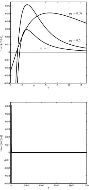
0 2 4 6 8 10
0 0.5 1 1.5 τ m a x ( R e ( λ ))
µ= 0.1
µ= 0.8
0 2000 4000 6000 8000 10000 0 0.005 0.01 0.015 0.02 0.025 0.03 0.035 0.04 0.045 0.05 τ m a x ( R e ( λ ))
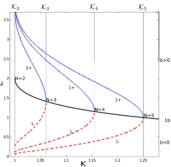
Figure 3.2: Real part of the rightmost root for the characteristic function PFix(SN)
with K = 2 and x∗
1 =φ+, forµ={0.1, 0.2, 0.4, 0.6, 0.8}.
0 2 4 6 8 10 12
−1.5 −1 −0.5 0 0.5 1 τ λ Real(λ)
Figure 3.3: Real part of the rightmost roots for the characteristic function PFix(SN)
with K = 2 and x∗
1 =φ+, forµ= 0.9 using DDE-Biftool.
Using the MatlabR
char-28 CHAPTER 3. FULL-PHASE MODEL acteristic roots converge when τ → ∞, see figure 3.3. Although roots can become stable when τ → ∞, we are interested only in finite values of time-delay; con-sequently, there is numerical evidence that some roots in PFix(SN) remain unstable
when x∗
1 =φ+ for any finite value of µ, τ ∈R+.
• For the equilibrium x∗
1 = φ− with K > 1, the characteristic function PFix(SN) in
equation (3.9) becomes
PFix(SN) =λ2+µλ+Kµ 1 + r
1− 1
K2 !
−Kµ 1−
r
1− 1
K2 !
e−λτ = 0.
From (3.12), we know both roots are stable when τ = 0 and, from (3.13), we also know there are no roots on the right-side of the complex plane when τ → ∞. From F(ω) = 0 in (3.15) with x∗
1 =φ−, we obtain
ω2
± = −
1 2 µ
2−2Kµ 1 + r
1− 1
K2 !!
±12
µ2−2Kµ 1 + r
1− 1
K2 !!2
−16K2µ2 r
1− 1
K2
1/2
.
Then, by Lemma 3.1 withc > 0, ω∈R+ if and only if the discriminant is positive and b <0, i.e., the first term is positive, which implies
µ <2K+√K2−1. (3.28)
The discriminant is positive if and only if
µ−2K+√K2−1>4 q
K√K2−1,
hence, by (3.28)
µ <2K+√K2−1−4 q
K√K2−1 =:µ
max, (3.29)
is a necessary condition for the existence of bifurcations in Fix(SN) when x∗
1 =φ−
with K >1. WhenK = 1, this condition becomes condition (3.25).
Remark. We know roots inPFix(SN) are stable whenx1∗ =φ− forK ≥1atτ = 0, see
(3.12); using the time-delay as parameter, bifurcations can occur for time delays τ
satisfying (3.20) provided condition (3.29) holds. If condition (3.29) does not hold, then roots of PFix(SN) will remain stable for allτ. In that sense, µmax sets the lower
limit toµfor the stability of the equilibrium inFix(SN)for all time delays τ in this
3.2. SYMMETRY-PRESERVING BIFURCATIONS 29
0 0.05 0.1 0.15 0.2 0.25 0.3 0.35 0.4 0.45 0
10 20 30 40 50 60
n=4 n=5 n=6
Figure 3.4: Symmetry-preserving bifurcation curves for the equilibrium x∗
1 = φ−,
with K = 1.05. Within the shadowed region, there are no roots with positive real part.
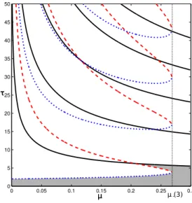
As an example, we choose K = 1.05; with this value, condition (3.29) becomes 0 < µ < µmax = 0.4211. With these parameters and using (3.16), (3.19), (3.20),
and (2.19), for x∗
1 =φ−, curves corresponding to τ± are presented in figure 3.4 for
different values of n (τ+ in solid line and τ− in dashed line), a lobe τ+(n) andτ−(n)
is plotted for each n; note that only positive values ofτ are considered. We already know from (3.23) thatδ+(ω+)>0andδ−(ω−)<0, thus the shadowed area indicates
the region where the equilibrium is stable in Fix(SN).
These results are tested using DDE-Biftool (Engelborghs et al., 2002, 2001); with
µ = 0.3 and K = 1.05, we found the critical time delays τ1 to τ5 leading to Hopf
bifurcations (τ1 = 6.34, τ2 = 11, τ3 = 15.41, τ4 = 23.51, and τ5 = 24.48) which
match with those found using the Sn map, see figure 3.4. In figure 3.5, the real
part of the rightmost root is shown as a black curve, and the critical time delays τ1
to τ5 are also shown. Each peak is related to the corresponding lobe in figure 3.4;
the numerics confirms that at τ1, τ3 and τ5, the rightmost root crosses from the
left to the right of the imaginary axis switching stability from stable to unstable and, at τ2, τ4, the rightmost root come back to the left-hand side of the complex
30 CHAPTER 3. FULL-PHASE MODEL in Fix(SN). Thus, for the given parameters the equilibrium is stable in Fix(SN)
within the interval (0, τ1)∪(τ2, τ3)∪(τ4, τ5), when µ < µmax.
10 20 30 40 50 60
−0.035 −0.03 −0.025 −0.02 −0.015 −0.01 −0.005
0 0.005 0.01
τ Re(λ)
n=1 n=2
n=3
n=4 n=5
n=6
Figure 3.5: Real part of the rightmost root ofPFix(SN)forx∗1 =φ−,µ= 0.3, andK = 1.05,
using DDE-Biftool.
3.3
Symmetry-breaking bifurcations
In this section we shall analyze conditions for existence of bifurcations in Wj.
3.3.1
Roots in the characteristic function
P
jat
τ
= 0
and as
τ
→ ∞
Seeing that K ≥ 1, N ∈ N > 1 and µ ∈ R+, we have that the characteristic function
Pj(λ, τ, η)in (3.9) when τ = 0 becomes
Pj(λ,0, η) = λ2+µλ+Kµ(1−cos(2x∗1)) +
Kµ
N −1(1 + cos(2x
∗
1)) = 0,
whose roots are
λ±=−µ 2 ±
1 2
µ2−4Kµ
1−cos(2x∗1) + 1
N −1(1 + cos(2x
∗
1)) 1/2
;
since |cos(2x∗
1)|<1, see (3.10), the discriminant is always smaller than µ2; consequently,
3.3. SYMMETRY-BREAKING BIFURCATIONS 31 When τ → ∞, assuming Re(λ)>0in (3.9), we obtain,
lim
τ→∞λ± =− µ
2 ± 1 2 µ
2
−4Kµ(1−cos(2x∗1)) 1/2
,
here again the discriminant is always smaller thanµ2; thus,Re(λ±)<0, which contradicts
the assumption Re(λ) > 0, and the roots of Pj are therefore not on the right-hand side
of the complex plane whenτ → ∞. These results are valid for both equilibriax∗
1 =φ±.
3.3.2
Conditions for the existence of symmetry-breaking
bifurc-ations
For the characteristic function Pj in (3.9), following (2.12), we have
R(λ, η) = λ2+µλ+Kµ(1−cos(2x∗
1))
S(λ, η) = Kµ
N −1(1 + cos(2x
∗
1)),
and substitutingλ = iω we obtain
R(iω, η) = −ω2+Kµ(1−cos(2x∗
1)) + iµω
S(iω, η) = Kµ
N −1(1 + cos(2x
∗
1)),
(3.30)
thus the polynomialF(ω) from (2.15) becomes
F(ω) = ω4+ (µ2−2Kµ(1−cos(2x∗
1)))ω2
+(Kµ)2(1−cos(2x∗
1)) 2
−
Kµ N −1
2
(1 + cos(2x∗
1)) 2
= 0, (3.31)
from which we get
ω2
± = −
1 2(µ
2−2Kµ(1−cos(2x∗
1)))
±12
"
(µ2−2Kµ(1−cos(2x∗
1))) 2
−4
(
(Kµ)2(1−cos(2x∗
1)) 2
−
Kµ N−1
2
(1 + cos(2x∗
1)) 2
)#1/2
.
(3.32)
For the sake of simplicity we write
ω± =
r
−2b ± 12√b2−4c, (3.33)
where
b = µ2−2Kµ(1−cos(2x∗
1))
c = (Kµ)2(1−cos(2x∗
1))2−
Kµ N −1
2
(1 + cos(2x∗
1))2.
32 CHAPTER 3. FULL-PHASE MODEL The first necessary condition for the existence of bifurcations in Wj is (3.18), then
sub-stituting b and cin this condition we obtain
µ2 −4µK(1−cos(2x∗
1)) +
2K N −1
2
(1 + cos(2x∗
1))2 ≥ 0.
By calculating the real roots of this equation, it is possible to find the boundaries in which this inequality holds true; these real roots follow two curves depending on K with N as parameter,
µ±(K;N) =
2K(1−cos(2x∗
1))±2K "
(1−cos(2x∗
1)) 2
−
1
N −1
2
(1 + cos(2x∗
1))2 #1/2
. (3.35)
Note that the discriminant is always smaller than the square of the first term; therefore,
µ±∈R+. The set M of all valuesµ satisfying condition (3.18) is
M ={µ∈R+/µ ∈ {h0, µ−]∪[µ+,+∞i}}. (3.36)
Additional necessary conditions for the existence of Hopf bifurcations are given in Lemma 3.1. Condition b ≥0 is equivalent to
µ≥2K(1−cos(2x∗1)), (3.37) and condition c >0 means
(N −1)2(1−cos(2x∗
1)) 2
−(1 + cos(2x∗
1))2 >0,
here, since all factors are greater than zero, this is equivalent to
N −2
N >cos(2x ∗
1). (3.38)
Now, we will analyze conditions for the existence of bifurcations in Wj considering three
cases:
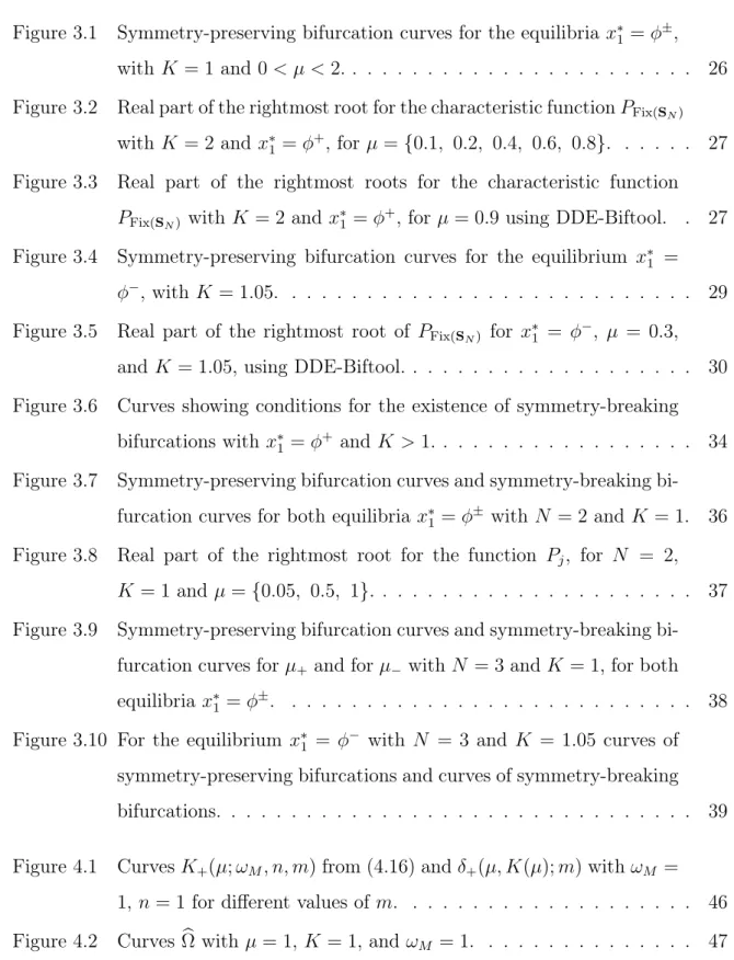
• When K = 1, we havecos(2x∗
1) = 0, see (3.10); thus, the following analysis will be
valid for both equilibria x∗
1 =φ±1. For this case, curves µ± from (3.35) become
µ±(1;N) = 2± 2
N −1
p
N(N −2), (3.39)
clearly, for N ∈N>1we obtain