A
A
ARE
LEVERAGE
AND
DEBT
MATURITY
COMPLEMENTS
OR
SUBSTITUTES
?
EVIDENCE
FROM
LATIN
AMERICA
A ALAVANCAGEM E A MATURIDADE DO ENDIVIDAMENTO SÃO COMPLEMENTARES OU SUBSTITUTOS? EVIDÊNCIA DA AMÉRICA LATINA
PAULO RENATO SOARES TERRA
Doutor em Administração, McGill University, Canadá. Professor adjunto de Finanças do Programa de Pós-Graduação em Administração da
Universidade Federal do Rio Grande do Sul (UFRGS). Rua Washington Luís, 855, sala 321 – Porto Alegre – RS – Brasil – CEP 90010-460
E-mail: prsterra@ea.ufrgs.br
5
A B S T R A C T
The aim of this paper is to investigate the choice between debt and equity simul-taneously with the decision between short- and long-term debt for a large sample of emerging markets from Latin America. In order to do this, we test a model (BARCLAY; MARX; SMITH JR., 2003) of joint capital structure and debt maturity determination for a sample of 986 firms from Latin America in the period 1990-2002, employing the Generalized Method of Moments on a system of equations. The empirical results support three main findings. First, capital structure and debt maturity are financial policy complements in Latin America. Second, there is a substantial dynamic component in the determination of debt maturity that has been neglected by previous research. Finally, firms face moderate adjustment costs towards their optimal maturity. Results are robust to variation in sample composi-tion in terms or countries, industries, and years.
K E Y W O R D S
Capital structure; Debt maturity; Trade-off, Dynamic panel data analysis; Latin America.
R E S U M O
Segun-6
do, há um componente dinâmico substancial na determinação da maturidade do endividamento que tem sido negligenciado por pesquisas anteriores. Finalmente, as empresas enfrentam moderados custos de ajuste em direção à sua maturidade ótima de endividamento. Os resultados são robustos à variação na composição da amostra em termos de países, setores e anos.
P A L A V R A S - C H A V E
Estrutura de capital; Maturidade da dívida; Trade-off; Análise dinâmica de dados em painel; América Latina.
1
I N T R O D U C T I O N
Since the breakthrough work of Modigliani and Miller (1958, henceforth MM) on capital structure, corporate financial theory has furthered our unders-tanding of a range of financial decisions: the choice between debt and equity, the design of a payout policy, the use of convertible instruments, and the mana-gement of financial risks, among others. In their influential paper and the ones that followed (MILLER; MODIGLIANI, 1961; MODIGLIANI; MILLER, 1963; MILLER, 1977), these authors laid down the conditions under which the firm would be largely indifferent to the sources of its financing. In the fifty years that followed the publication of their work, several papers have explored both theo-retically and empirically the implications of their famous Propositions I, II and III. Capital structure and dividend policy are perhaps the most studied issues in corporate finance. Much less attention however has been devoted to the maturity structure of the firm’s financing. Moreover, most of the theoretical and empiri-cal work so far has focused on a single decision at a time. That is, each financial decision is taken as independent of the other decisions. It may be the case that some of these decisions are not independent but actually complements or substi-tutes among each other. If that is the case, we must investigate whether there is interdependence among them or not.
7
empirical techniques that account properly for cross-section and time series variation. Also, we model dynamic effects that have not been considered in the original research.
Our main findings suggest that there is a substantial dynamic component in the determination of a firm’s maturity structure, which has been ignored by previous research. Moreover, our results suggest that capital structure and debt maturity are policy complements in Latin America, an empirical finding that con-tradicts Barclay, Marx, and Smith Jr.’s (2003) theoretical prediction. The study also finds that firms face moderate adjustment costs towards its optimal policies.
The remaining of the paper is organized as follow: the next section lays down the theoretical underpinnings of the joint capital structure/debt maturity decision. Section 3 presents the data sources, the variables, the model, describes the sample, and the empirical techniques. Section 4 presents and discusses the findings. The last section summarizes the results and concludes the paper.
2
T H E O R E T I C A L F R A M E W O R K A N D
P R E V I O U S E M P I R I C A L E V I D E N C E
Theoretical explanations for the choice of corporate debt maturity are alre-ady implied in MM’s original paper, but are eventually formalized by Stiglitz (1974). MM’s paper does not consider a multi-period setting, and Stiglitz (1974) provides a rigorous analysis of their model in such circumstances. His conclu-sions are that, under a fairly general set of conditions (absence of taxation, tran-saction costs, bankruptcy costs, and other market frictions) the maturity choice of the firm is irrelevant, just as MM’s findings regarding the firm’s leverage ratio under the same conditions. Of course, once one departs from the ideal world of the financial economists1, such frictions matter, and therefore the maturity deci-sion would influence the firm’s valuation just as would the set of other financial policies. A large family of hypotheses explores the tax-based, bankruptcy costs, and transaction costs approaches in order to offer an explanation for the maturity choice.
Barclay, Marx, and Smith Jr. (2003) propose the requirements for a theory of financial policy to have testable implications. The authors focus their work on the choice between leverage and maturity. They develop their model from the argument that a firm chooses leverage and debt maturity to maximize its value given a set of exogenous firm characteristics such as its investment opportunity
8
set and regulatory status. In order to obtain unambiguous predictions in reduced form equations, the value functions must have monotone comparative statics, which is guaranteed only if particular properties are satisfied (single-crossing and quasi-supermodularity).
The term “single crossing” is used because the objective function crosses zero only once (and only from below) when this condition holds (MILGROM; SHANNON, 1994). Milgrom and Shannon (1994) remark that not only is the sin-gle crossing property a condition describing the relationship between the choice variables and the parameters, but it is also an ordinal condition. Simply put, “the single crossing property says that, if a given increase in the decision variable is profitable when the parameter is low, the same increase will continue to be profitable when the parameter is high” (AMIR, 2005, p. 636). Moreover,
[...] quasi-supermodularity expresses a weak kind of complementarity between the choice variables; if an increase in some subset of the choice variables is desi-rable at some level of the remaining choice variables, it will remain desidesi-rable as the remaining variables also increase (MILGROM; SHANNON, 1994, p. 162).
Thus, single crossing is a weaker property than quasi-supermodularity. Bar-clay, Marx, and Smith Jr. (2003) show that, for the leverage-maturity problem, the single crossing property holds, but the quasi-supermodularity one does not. The practical implication is that leverage and debt maturity are likely to be subs-titute policies instead of complementary ones. Complementarity can be defined as mutually reinforcing increases in the case of multiple endogenous variables (AMIR, 2005), while substitutability can be defined as increases in one of the endogenous variables replaces increases in other endogenous variables. In other words, firms facing restrictions in their level of leverage (e.g. borrowing restric-tions) may make up for it by extending the maturity of their debt and vice-versa. Barclay, Marx, and Smith Jr. (2003) illustrate their point empirically using data from 5,765 industrial firms in the United States from 1980 to 1999. Besi-des endogenous variables for capital structure and debt maturity, the authors employ exogenous variables such as growth opportunities, industry regulation, firm size, profitability, tangibility, asset maturity, average tax rate, net-ope-rating loss carryforwards, and a dummy variable for firms with commercial paper programs. Their empirical analysis suggests that capital structure and debt maturity are substitutes in addressing financial problems of the firms although the authors have faced several difficulties in correctly identifying the leverage equation.
9
international setting. Antoniou, Guney, and Paudyal (2006) study the determi-nants of debt maturity for a sample of 358 French, 582 German, and 2,423 British non-financial firms and find that debt maturity depends on both firm-specific and country-specific factors, opening the question of the degree of influence of each group of factors on the maturity structure. Larger sets of countries are studied by Demirgüç-Kunt and Maksimovic (1999) who explored the hypothesis that the financial development of a country determines the maturity of its firms’ debt. The authors investigate 9,649 non-financial firms from 30 countries including developing ones in the period 1980-1991. They find support for the hypothesis that legal and institutional differences among countries explain a large part of the leverage and debt maturity choices of firms. Fan, Titman, and Twite (2008) also study the subject for 11 industries in 39 countries in the period 1991-2006. Their results largely support Demirgüç-Kunt and Maksimovic (1999) findings.
To the best of our knowledge, so far, the only study that focused specifi-cally on developing countries is Erol (2004), who analyzed the strategic content of debt maturity in a sample of 15 manufacturing sectors from Turkey during the period 1990-2000. The author’s findings are that long-term debt is strategic while short-term debt, despite being devoid of strategic content, is associated with financial constraint. Erol (2004), however, limits his analysis to a single emerging market.
Besides most of previous empirical studies having neglected multi-country emerging markets samples, one criticism that may be raised against Barclay, Marx, and Smith Jr.’s (2003) paper is that it ignores the effect that lagged leverage and maturity may have on the determination of the contemporaneous endogenous variables. As a matter of fact, it is likely that the change in a firm’s capital structure and debt maturity is somewhat rigid and by no means costless. If that is the case, the previous period’s level of debt and maturity is a relevant variable in the firm’s choice today. These are particular aspects that we intend to improve in the empi-rical analysis that follows. In the next section, we describe the methods, variables, and data we employ in order to investigate the joint capital structure debt maturity decision of non-financial firms in the seven biggest economies of Latin America.
3
D A T A , V A R I A B L E S , M O D E L , A N D
E M P I R I C A L M E T H O D S
3 . 1
D ATA A N D VA R I A B L E S10
America has experienced hyperinflation and economic instability over the 1980s and profound economic reforms in the 1990s, including extensive privatization programs.
The primary data sources are from the Economática Pro© database for Latin American countries (ECONOMÁTICA, 2003). Only listed firms are included in the sample. Observations are yearly during the period 1990-2002 the level of analysis is each firm. The database contains 1,242 firms over the period covered. Firms from the financial industry were excluded as well as firms with missing data for key variables. Thus, the final sample contains 986 firms and 13,490 observations from Latin America. In order to reduce the survival bias, firms are allowed to leave and enter the dataset over time. Firms are classified in 19 indus-try sectors, according to their primary NAICS codes. Panel A of Table 1 presents the distribution of firms and observations by country. We highlight the share of Brazilian firms in the sample, making up more than 40% of the firms and slightly less of the observations. In the other extreme is Venezuela, with only 28 firms in the sample and less than 3% of the observations.
TABLE 1
SUMMARY STATISTICS FOR ENDOGENOUS VARIABLES*
PANEL A: FIRMS BY COUNTRY
COUNTRIES FIRMS %
Argentina 76 7.7
Brazil 395 40.1
Chile 169 17.1
Colombia 47 4.8
Mexico 145 14.7
Peru 126 12.8
Venezuela 28 2.8
Latin America 986 100.0
11
PANEL B: DESCRIPTIVE STATISTICS BY COUNTRY
COUNTRIES
LEVERAGE MATURITY
OBS. MEAN STD. DEV. OBS. MEAN STD. DEV.
Argentina 614 0.9552 6.7349 538 0.4184 0.3283
Brazil 3270 1.6999 15.1451 2850 0.4645 0.3078
Chile 1742 0.3266 0.6098 1518 0.4997 0.3540
Colombia 280 0.4687 1.7781 241 0.4617 0.3410
Mexico 1324 0.6869 1.2427 1204 0.5431 0.3227
Peru 1012 1.0447 19.5014 142 0.4012 0.3392
Venezuela 175 0.2757 0.3367 146 0.4292 0.3112
Latin America 8417 1.0527 11.7826 6639 0.4808 0.3272
*The sample consists of 13,490 observations for firms of Argentina, Brazil, Chile, Colombia,
Mexi-co, Peru and Venezuela (ECONOMÁTICA, 2003) over the period 1990-2002. Leverage is calculated as the book value of long-term debt over book value of equity. Maturity is the book value of long-term financial debt over book value of short-term loans plus book value of long-term financial debt. “Latin America” refers to the pooling together of all firm-level data for Argentina, Brazil, Chile, Colombia, Mexico, Peru, and Venezuela.
Source: Elaborated by the author.
The endogenous variables are proxies of the leverage and maturity of debt carried by each firm measured as follows: Long-Term Book Debt over Book Equity, i.e., the debt-to-equity ratio (“Leverage”), and Long-Term Financial Debt over Short-Term Loans plus Long-Term Financial Debt (“Maturity”).
Panel B of Table 1 shows the summary statistics for Leverage and Maturity
variables, respectively. Brazil has the most leveraged firms in average, while Venezuelan firms are the least indebted ones in the sample. The high variation of the debt-to-equity ratios of Peruvian firms stands out. Maturities, on the other hand, are much more homogeneous both within and across countries. Mexico presents firms with longer debt maturities while Peru has the shortest ones.
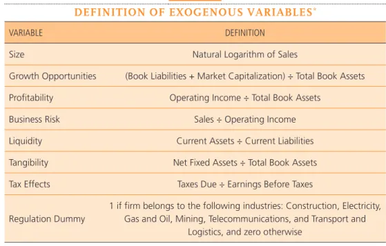
Firm-specific determinant factors for the debt maturity structure are chosen from those often suggested in the literature. The set of firm-specific explanatory variables consists of the following: size, growth opportunities, profitability, busi-ness risk, liquidity, tangibility, tax effects, and a dummy variable to control for regulated industries. The measurement of such variables is presented in Picture 1, and it is standard in the extant literature.
TABLE 1 (CONTINUATION)
12
PICTURE 1
DEFINITION OF EXOGENOUS VARIABLES*
VARIABLE DEFINITION
Size Natural Logarithm of Sales
Growth Opportunities (Book Liabilities + Market Capitalization) ÷ Total Book Assets
Profitability Operating Income ÷ Total Book Assets
Business Risk Sales ÷ Operating Income
Liquidity Current Assets ÷ Current Liabilities
Tangibility Net Fixed Assets ÷ Total Book Assets
Tax Effects Taxes Due ÷ Earnings Before Taxes
Regulation Dummy
1 if firm belongs to the following industries: Construction, Electricity, Gas and Oil, Mining, Telecommunications, and Transport and
Logistics, and zero otherwise
*Exogenous variables are computed based in accounting and stock market data provided by the
Economática Pro© database (2003) over the period 1990-2002.
Source: Elaborated by the author.
Table 2 reports summary statistics for the exogenous variables of Latin Ame-rican firms. Inspecting the table, we can conclude that Argentine firms are the most profitable and have the lower risk2 but are the least liquid; Brazilian firms are the most heavily taxed of the continent; Chilean firms are the most valuable in the market; Colombia have the riskier and the least profitable firms, and those with less tangible assets; Mexican firms are bigger and more liquid, but have the lowest average taxation; Peruvian firms are the smallest, Venezuela have firms with more tangible assets but the least valuable. Overall, standard deviations of such variables at the firm level are very high both within and across countries.
Finally, we also define a dummy variable to control for regulated industries. This variable assumes the value of 1 if the firm’s main industrial activity belongs to one of the following industries: Construction, Electricity, Gas and Oil, Mining, Telecommunications, and Transport and Logistics. These industries are subject to closer government scrutiny even when pursued solely by private enterprises, and are submitted to stricter regulations than other activities.
2 Notice that our sample period ends in 2002, before the meltdown of the Argentine currency board regime
13
TABLE 2
SUMMARY STATISTICS FOR EXPLANATORY VARIABLES*
COUNTRIES ARGENTINA BRAZIL CHILE COLOMBIA
VARIABLES OBS. MEAN STD. DEV OBS. MEAN STD. DEV OBS. MEAN STD. DEV OBS. MEAN STD. DEV
Size 582 11.3880 1.8235 2896 11.5804 1.8322 1580 10.2488 1.8960 297 11.0402 1.5650
Growth
Opportunities 497 0.9887 0.4354 2813 0.8115 0.4786 1320 2.1829 8.6707 201 0.8253 0.4274
Profitability 614 0.3538 0.0711 3262 0.0308 0.8922 1748 0.05872 0.1025 287 0.0303 0.0781
Business Risk 594 0.8755 155.6350 3253 1.2234 155.8223 1633 12.7145 125.3976 286 31.1815 725.7262
Liquidity 614 1.6938 2.7358 3263 2.5267 22.5466 1738 5.0646 43.2245 281 1.6976 1.1712
Tangibility 597 0.4597 0.2619 3265 0.3578 0.2621 1719 0.4111 0.2879 274 0.2494 0.1894
Tax Effects 344 0.1399 1.0425 3260 0.4042 12.4357 1482 0.0295 0.8842 287 0.1107 1.5110
COUNTRIES MEXICO PERU VENEZUELA LATIN AMERICA
VARIABLES OBS. MEAN STD. DEV OBS. MEAN STD. DEV OBS. MEAN STD. DEV OBS. MEAN STD. DEV
Size 1335 12.2981 1.7981 1005 10.2201 1.2713 166 10.9196 1.8189 7861 11.2121 1.9207
Growth
Opportunities 873 1.2778 0.6577 633 1.1085 0.7247 140 0.7463 0.3507 6477 1.1955 3.9775
Profitability 1339 0.0756 0.7630 1010 0.0597 0.1178 175 0.0346 0.0659 8435 0.0475 0.0938
Business Risk 1339 16.8693 196.8102 1006 14.8608 267.0739 171 2.1902 51.4443 8282 8.7048 218.0081
Liquidity 1340 5.2687 99.4697 1012 2.0033 4.2355 175 2.1203 2.8290 8423 3.3263 46.4780
Tangibility 1340 0.5120 0.2716 1012 0.4771 0.2220 175 0.5355 0.2263 8382 0.4152 0.2705
Tax Effects 1339 -4.1846 137.5319 1009 0.3121 3.9597 174 0.0971 1.5772 7895 -0.4851 57.2277
*The sample consists of 13,490 observations for firms of Argentina, Brazil, Chile, Colombia, Mexico,
Peru and Venezuela (ECONOMÁTICA, 2003) over the period 1990-2002. Size is the natural loga-rithm of sales. Growth Opportunities is equal as the book value of liabilities plus market capitalization over book value of total assets. Profitability is equal to operating income over book value of total assets. Business Risk is calculated as sales over operating income. Liquidity is book value of current assets over book value of current liabilities. Tangibility is defined as net fixed assets over book value of total assets. Tax Effects is equal to taxes due over earnings before taxes. “Latin America” refers to the pooling together of all firm-level data for Argentina, Brazil, Chile, Colombia, Mexico, Peru, and Venezuela.
Source: Elaborated by the author.
14
TABLE 3
CORRELATION MATRICES*
SIZE GROWTH
OPPORTUNITIES PROFITABILITY
BUSINESS
RISK LIQUIDITY TANGIBILITY TAX EFFECTS
Size 1.0000
Growth
Opportunities 0.0696 1.0000
Profitability 0.2085 0.0233 1.0000
Business Risk 0.0116 -0.0016 0.0110 1.0000
Liquidity -0,0060 -0,0243 -0.0177 -0.1498 1.0000
Tangibility 0.1652 0.0568 0.1169 0.0070 -0.0505 1.0000
Tax Effects -0.0200 -0.0008 0.0039 -0.0028 0.0003 -0.0028 1.0000
*The table presents the correlation matrix for firms in Latin America, and refers to the pooling together of all firm-level data for Argentina, Brazil, Chile, Colombia, Mexico, Peru, and Venezuela in the period 1990-2002.
Source: Elaborated by the author.
3 . 2
M O D E L A N D E M P I R I C A L M E T H O D SWe specify the model as the following general (static) panel data model:
(Eq. 1)
Where Leverageit and Maturityit are the endogenous variables (the ith-firm leverage and maturity ratios on the tth-period), Y
it are the K firm-specific explana-tory variables, (including industry dummies in the simple pooling and random-effects models), Zit is the matrix of L country dummies (in the simple pooling and random-effects models),βi and γi are the firm-specific intercepts in the fixed-effects model, βt and γt are period-specific intercepts,βk, βl, γk and γl are the exo-genous variables coefficients to be estimated,ηi and ωi are the firm-specific error terms in the random-effects model, and εit and νit are the error terms.
15
that the debt policy of the firm may be dynamic, i.e., current leverage and matu-rity may depend on past leverage and matumatu-rity. Antoniou, Guney, and Paudyal (2006) explicitly model such possibility, and suggest that a dynamic rather than static panel data analysis may be more adequate. The next step then is to test then the lagged endogenous variable is added to Eq. 1, which is then first-diffe-renced yielding the dynamic system below:
(Eq. 2)
Where β0 and γ0 are the endogenous variables coefficients to be estimated. One advantage of this specification is that the rate of adjustment of the firm towards its optimal capital structure and maturity can be estimated respectively as λ1 = (1 – β0) and λ2 = (1 – γ0). If adjustment costs are high, the rate of adjust-ment is expected to be small (λ approaching zero), while a very high rate of adjustment (λ approaching one) suggests the presence of negligible adjustment costs.
16
4
E M P I R I C A L
R E S U L T S
4 . 1
P R E L I M I N A R Y S P E C I F I C AT I O N T E S T SThe first step is to determine whether the panel data specification that sim-ply pools together all available data for all firms and time periods is adequate to describe the data3. As pointed out by Hsiao (1986), simple least squares estima-tion of pooled cross-secestima-tion and time series data may be seriously biased4. The model tested in Eq. 1 includes firm-specific variables described above, as well as country-specific dummy variables. The results in Table 4 strongly reject the single intercept hypothesis.
TABLE 4
SPECIFICATION TESTS*
PANEL A: F TEST PANEL B: HAUSMAN TEST
LEVERAGE MATURITY LEVERAGE MATURITY
F(714; 3908) F(714; 3908) χ2(4) χ2(13)
2.0101* 4.9446* 101.960* 16.864
0.000 0.000 0.000 0.206
*PANEL A presents the F-Test of a Simple Pooled OLS against a Fixed-Effects Specification. This test statistic is for testing the null hypothesis that firms’ intercepts in the basic fixed-effects panel data model are all equal, against the alternative hypothesis that each firm has its own (distinct) inter-cept. The test assumes identical slopes for all independent variables across all firms, and it is dis-tributed F(df1, df2). PANEL B presents the Hausman Specification Test of Random-Effects against Fixed-Effects Specification. This test statistic is for testing the null hypothesis of the random-effects specification against the alternative hypothesis of the fixed-effects specification in the basic panel data model, and it is distributed χ2(df). The sample refers to the pooling together of all firm-level data for
Argentina, Brazil, Chile, Colombia, Mexico, Peru, and Venezuela. Endogenous Variables: Leverage = Long-Term Book Liabilities ÷ Book Equity; Maturity = Long-Term Debt ÷ Total Debt. p-values in italic. * Significant at the 1% level.
Source: Elaborated by the author.
The next step is to determine which model of variable intercepts across firms better fits the data. Table 4 also presents the results for a Hausman specification test of random-versus fixed-effects. The test, as suggested by Hsiao (1986, p. 49), is
3 Such tests are not strictly required to implement the dynamic model, but they are reassuring in that the
first differences model is indeed adequate.
17
particularly appropriate in situations where N (the number of cross-sectional units) is large relative to T (the number of time periods) – precisely the case of this study. Again, the model in Eq. 1 is employed. The test rejects the random-effects specifica-tion for the leverage equaspecifica-tion but cannot reject it for the maturity equaspecifica-tion.
Given these results, after first differencing Eq. 1, firm-specific intercepts dis-appear. Random-effects, however, are not likely to disappear with differencing and are incorporated to the general error term in the dynamic model of Eq. 2 in the estimation that follows.
4 . 2
DY N A M I C PA N E L D ATA E S T I M AT I O N R E S U LT SAs mentioned above, usual OLS and GLS estimators are biased and incon-sistent when the lagged dependent variable is included in the right-hand side of the panel data model. In order to overcome this problem, GMM estimation is used instead.
The Eq. 2 is then estimated by Generalized Method of Moments (GMM) using as instruments first-order lagged values of the levels5 of explanatory varia-bles, sector dummies, country dummies, and a constant. Standard errors are heteroskedasticity robust according to the method proposed by White (1980)6 and are also robust to autocorrelation. Results are reported in Table 5.
TABLE 5
PANEL DATA ANALYSIS OF MATURITY RATIOS FOR LATIN AMERICA*
ENDOGENOUS VARIABLES
EXPLANATORY VARIABLES ↓ LEVERAGE MATURITY
ΔLeveraget 0.0262
6.9861
***
ΔMaturityt 15.8237
8.9450
***
ΔLeveraget–1 0.3281
1.2109
–0.0039
–0.6735
ΔMaturityt–1 –5.8078
–6.0183
*** 0.3679
8.8230
***
5 As suggested by Arellano (1989).
6 Given the heterogeneity of the firms in the sample, we anticipate that heteroskedasticity might be a problem.
18
ENDOGENOUS VARIABLES
EXPLANATORY VARIABLES ↓ LEVERAGE MATURITY
ΔSize t 2.0690
2.5093
** –0.1089
–2.6423
***
ΔGrowth Opportunities t 0.3043
0.7780
–0.0153
–0.6760
ΔProfitability t –1.2305
–0.3338
0.1477
0.8179
ΔBusiness Risk t 0.0005
1.3408
0.0000
–1.5770
ΔLiquidity t –0.5759
–3.1660
*** 0.0329
2.5854
***
ΔTangibility t –5.6540
–1.3894
0.2333
1.1477
ΔTax Effects t 0.0015
3.5933
*** –0.0001
–3.9366
***
Regulation Dummy –0.0238
–0.1707
0.0018
0.2446
Number of Observations Adjusted R2
F-statistic F[df1; df2]
3,305 –0.0027 0.1145 [10; 3294]
3,305 0.0053 2.7712 [10; 3294]
***
Sargan’s Test Statistic (p-value) χ2[df] 26.7493 (0.986) [45] *First-differences model so that idiosyncratic firm-effects constant through time are eliminated. The model is estimated by Generalized Method of Moments (GMM) using as instruments first order lagged values of the levels of explanatory variables, industry dummies, country dummies, and a constant. Estimation in the period 1990-2002. “Latin America” refers to the pooling together of all firm-level data for Argentina, Brazil, Chile, Colombia, Mexico, Peru, and Venezuela. Endo-genous Variables: Leverage = Long-Term Book Liabilities ÷ Book Equity; Maturity = Long-Term Debt ÷ Total Debt. Reported t-statistics are calculated using heteroskedasticity-robust standard errors (White) and are also robust to autocorrelation (Bartlett Kernel). t-statistics in italic; degrees of freedom in (brackets); p-values in (square brackets).
** Significant at the 5% level. *** Significant at the 1% level.
Source: Elaborated by the author.
TABLE 5 (CONTINUATION)
19
One important issue when estimating via GMM is to make sure that the instrument set is adequate. Table 5 reports the Sargan’s test statistic for the null hypothesis that moment restrictions are orthogonal. Results cannot reject the restrictions. Therefore, we conclude that the instrument set is valid.
The first empirical result is that both specifications explain very poorly both the leverage and the maturity of the sample. The maturity equation performs slightly better though. Another interesting result is that dynamic effects are significant for the maturity but not for the leverage equation. This indicates that firms face adjustment costs, albeit moderate, in the debt maturity decision, but not as much in the capital structure decision.
The result of most interest is the relationship between leverage and maturity as endogenous variables. Both are significantly positive determinants of each other in the Latin American sample. This finding indicates that these policy variables are likely complements instead of substitutes, contradicting the theore-tical prediction suggested by Barclay, Marx, and Smith Jr. (2003). One possible explanation for this result is that, given the particular institutional and economic environments of Latin America, bigger firms in these markets (of which the lis-ted companies of our sample are an example) obtain a financial advantage that allows them to use financing alternatives in their favor, thus reinforcing each other.
Regarding the remaining explanatory variables, Size is found significant and positive in the leverage equation and significantly negative in the maturity equa-tion. Liquidity, on the other hand, as a significantly negative effect on leverage but a positive one in maturity (i.e., more liquid firms choose less and longer debt). Tax Effects are significantly positive in leverage and negative in maturity, indicating that more heavily taxed firms choose a higher level of indebtedness and shorter maturity, which is in line with the static-trade-off explanation of capi-tal structure. The remaining variables are not significant. It is worth to undersco-re that the two variables pointed out by Barclay, Marx, and Smith Jr. (2003) as the major theoretical determinants of the joint decision, Growth Opportunities and the Regulation dummy, are not significant in any equation and sample.
4 . 3
S E N S I T I V I T Y A N A LY S E S20
the results by dropping all observations of a given year at a time, and that of a single industry by dropping all firms of an industry at a time. The results are reported in Figures 1 to 4.
Results of these sensitivity analyses in general support the robustness of the previous findings. Average coefficients for independent variables are similar to the results reported above, and so are the t-statistics. In particular, the significance is in general confirmed in the Leamer’s histograms for those variables that are significant in the whole sample analysis presented in Table 5 (lagged leverage and lagged maturity, contemporaneous leverage and maturity, size, liquidity, and tax effects).
We therefore conclude that results reported in this paper are robust to the choice of countries, period, and industries covered.
FIGURE 1
GLOBAL SENSITIVITY ANALYSIS FOR LEVERAGE EQUATION IN LATIN AMERICA (COEFFICIENTS)
Source: Elaborated by the author.
LAGGED LEVERAGE MATURITY LAGGED MATURITY SIZE
GROWTH OPTIONS PROFITABILITY BUSINESS RISK LIQUIDITY
1,50 1,00 0,50 0,00 -0,50
L A G G E D L E V E R A G E 20 15 10 5 0 Frequency 80,00 60,00 40,00 20,00 0,00 -20,00 -40,00 25 20 15 10 5 0 LAGGED LEVERAGE 20 15 10 5 0 Fr equency
-0,50 0,00 0,50 1,00 1,50 Mean = 0,3979 Std. Dev. = 0,24307 N = 38
4 MATURITY 25 20 15 10 5 0 Fr equency
-40,00 -20,00 0,00 20,00 40,00 60,00 80,00 Mean = 12,8919 Std. Dev. = 15,52552 N = 38
LAGGED MATURITY 20 15 10 5 0 Fr equency
-20,00 -10,00 0,00 10,00 20,00 Mean = -4,0115 Std. Dev. = 5,59716 N = 38
SIZE 14 12 10 8 6 4 2 0 Fr equency
-6,00 -4,00 -2,00 0,00 2,00 4,00 Mean = 1,3873
Std. Dev. = 1,62208 N = 38
5 0 GROWTH OPTIONS 30 25 20 15 10 5 0 Fr equency
-4,00 -2,00 0,00 2,00 4,00 Mean = 0,317
Std. Dev. = 0,86771 N = 38
PROFITABILITY 25 20 15 10 5 0 Fr equency
-10,00 0,00 10,00 20,00 30,00 Mean = 1,6742 Std. Dev. = 7,07646 N = 38
BUSINESS RISK 30 25 20 15 10 5 0 Fr equency
-0,008 -0,006 -0,004 -0,002 0,00 0,002 0,004 Mean = 7,4864E-6
Std. Dev. = 0,00162 N = 38
LIQUIDITY 25 20 15 10 5 0 Fr equency
-3,00 -2,00 -1,00 0,00 1,00 2,00 Mean = -0,446 Std. Dev. = 0,72849 N = 38
TANGIBILITY TANGIBILITY 30 20 10 0 Fr equency
-150,00 -100,00 -50,00 0,00 50,00 Mean = -12,4827
Std. Dev. = 27,29316 N = 38
TAX RATE TAX RATE 30 25 20 15 10 5 0 Fr equency
-0,025 0,00 0,025 0,05 0,075 0,10 0,125 Mean = 0,0057 Std. Dev. = 0,02203 N = 38
REGULATION REGULATION 20 15 10 5 0 Fr equency
-0,60 -0,50 -0,40 -0,30 -0,20 -0,10 0,00 0,10 Mean = -0,0806
21
FIGURE 2
GLOBAL SENSITIVITY ANALYSIS FOR MATURITY EQUATION IN LATIN AMERICA (COEFFICIENTS)
Source: Elaborated by the author.
FIGURE 3
GLOBAL SENSITIVITY ANALYSIS FOR LEVERAGE EQUATION IN LATIN AMERICA (T-STATISTICS)
Source: Elaborated by the author.
0
LEVERAGE LAGGED LEVERAGE LAGGED MATURITY SIZE
GROWTH OPTIONS PROFITABILITY BUSINESS RISK LIQUIDITY
LEVERAGE 25 20 15 10 5 0 Fr equency
-0,03 -0,02 -0,01 0,00 0,01 0,02 0,03 0,04 0,05 Mean = 0,0156
Std. Dev. = 0,01613 N = 38
LAGGED LEVERAGE 15 12 9 6 3 0 Fr equency
-0,015 -0,01 -0,005 0,00 0,005 0,01 0,015 Mean = -3,9031E-4 Std. Dev. = 0,00687 N = 38
LAGGED MATURITY 20 15 10 5 0 Fr equency
0,10 0,20 0,30 0,40 0,50 0,60 Mean = 0,3611
Std. Dev. = 0,0591 N = 38
SIZE 14 12 10 8 6 4 2 0 Fr equency
-0,15 -0,10 -0,50 0,00 0,05 0,10 0,15 Mean = -0,0518 Std. Dev. = 0,08334 N = 38
GROWTH OPTIONS 30 25 20 15 10 5 0 Fr equency
-0,03 0,00 0,03 0,06 0,09 0,12 0,15 0,18 0,21 Mean = -9,958E-4 Std. Dev. = 0,03882 N = 38
PROFITABILITY 12 10 8 6 4 2 0 Fr equency
-0,60 -0,40 -0,20 0,00 0,20 0,40 0,60 Mean = 0,1476
Std. Dev. = 0,19115 N = 38
BUSINESS RISK 25 20 15 10 5 0 Fr equency
-2,00E-4 -1,50E-4 -1,00E-4 -5,00E-5 -2,711E-20 5,00E-5 1,00E-4
Mean = -1,5576E-5 Std. Dev. = 3,67847E-5 N = 38
LIQUIDITY 30 25 20 15 10 5 0 Fr equency
0,02 0,03 0,04 0,05 0,06 0,07 0,08 0,09 0,10 Mean = 0,0372 Std. Dev. = 0,01177 N = 38
TANGIBILITY
TANGIBILITY
Fr
equency
-1,00 -0,50 0,00 0,50 1,00 1,50 2,00 Mean = 0,1706
Std. Dev. = 0,44164 N = 38
TAX RATE TAX RATE 30 20 10 0 Fr equency
-2,00E-3 -1,50E-3 -1,00E-3 -5,00E-4 0,00E0 5,00E-4 Mean = -2,0875E-4
Std. Dev. = 4,3163E-4 N = 38
REGULATION REGULATION 25 20 15 10 5 0 Fr equency
-0,02 -0,01 0,00 0,01 0,02 0,03 0,04 Mean = 0,0015 Std. Dev. = 0,00778 N = 38 30 25 20 15 10 5 0
LAGGED LEVERAGE MATURITY LAGGED MATURITY SIZE
GROWTH OPTIONS PROFITABILITY BUSINESS RISK LIQUIDITY
LAGGED LEVERAGE 14 12 10 8 6 4 2 0 Fr equency
-2,00 -1,00 0,00 1,00 2,00 3,00 Mean = 1,4104
Std. Dev. = 0,71393 N = 38
LAGGED LEVERAGE 14 12 10 8 6 4 2 0 Fr equency
-10,00 0,00 10,00 20,00 30,00 Mean = 6,765 Std. Dev. = 6,65753 N = 38
LAGGED MATURITY 14 12 10 8 6 4 2 0 Fr equency
-7,5 -5,00 -2,50 0,00 2,50 5,00 Mean = -3,57 Std. Dev. = 3,40152 N = 38
SIZE 10 8 6 4 2 0 Fr equency
-1,00 0,00 1,00 2,00 3,00 4,00 5,00 Mean = 1,5776
Std. Dev. = 1,17599 N = 38
GROWTH OPTIONS 25 20 15 10 5 0 Fr equency
-2,00 -1,00 0,00 1,00 2,00 Mean = 0,4867
Std. Dev. = 0,58747 N = 38
PROFITABILITY 12 10 8 6 4 2 0 Fr equency
-2,00 -1,00 0,00 1,00 2,00 Mean = 0,0495 Std. Dev. = 0,81757 N = 38
BUSINESS RISK 20 15 10 5 0 Fr equency
-2,00 -1,00 0,00 1,00 2,00 3,00 Mean = 0,8379
Std. Dev. = 0,89372 N = 38
LIQUIDITY 15 12 9 6 3 0 Fr equency
-4,00 -3,00 -2,00 -1,00 0,00 1,00 2,00 Mean = -2,073 Std. Dev. = 1,67767 N = 38
TANGIBILITY
TANGIBILITY
Fr
equency
-5,00 -4,00 -3,00 -2,00 -1,00 0,00 1,00 Mean = -1,1115
Std. Dev. = 1,0356 N = 38
TAX RATE TAX RATE 25 20 15 10 5 0 Fr equency
-4,00 -2,00 0,00 2,00 4,00 6,00 Mean = 2,0556
Std. Dev. = 2,26409 N = 38
REGULATION REGULATION 20 15 10 5 0 Fr equency
22
FIGURE 4
GLOBAL SENSITIVITY ANALYSIS FOR MATURITY EQUATION IN LATIN AMERICA (T-STATISTICS)
Source: Elaborated by the author.
5
C O N C L U S I O N S
The aim of this paper is to investigate the choice between debt and equity simultaneously with the decision between short-and long-term debt for a large sample of firms from Latin America. To address this question, a sample of 986 non-financial firms from Latin America over a 14-year period is analyzed.
The empirical results support three main findings. First, cross-effects between capital structure and debt maturity suggest that these policy variables are likely complements in Latin America. Second, there is a substantial dynamic compo-nent in the determination of debt maturity, a factor that has been overlooked by previous research. Finally, firms face moderate adjustment costs towards their optimal maturity.
In spite of the results, the quality of measurement of the variables should be looked with some caution. As noted, accounting standards, financial market depth, and the degree of supervision on financial reporting may vary largely across countries which may harm the comparability of the results. Also, some
0 0 5 0 5 0
LEVERAGE LAGGED LEVERAGE LAGGED MATURITY SIZE
GROWTH OPTIONS PROFITABILITY BUSINESS RISK LIQUIDITY
LEVERAGE 15 12 9 6 3 0 Fr equency
-5,00 0,00 5,00 10,00 15,00 20,00 Mean = 5,378 Std. Dev. = 5,0165 N = 38
LAGGED LEVERAGE 15 12 9 6 3 0 Fr equency
-2,00 -1,00 0,00 1,00 2,00 3,00 4,00 Mean = 0,0224 Std. Dev. = 1,39645 N = 38
LAGGED MATURITY 14 12 10 8 6 4 2 0 Fr equency
0,00 2,00 4,00 6,00 8,00 10,00 Mean = 7,2647
Std. Dev. = 2,03872 N = 38
SIZE 15 12 9 6 3 0 Fr equency
-4,00 -3,00 -2,00 -1,00 0,00 1,00 2,00 Mean = -1,4009 Std. Dev. = 1,58235 N = 38
GROWTH OPTIONS 20 15 10 5 0 Fr equency
-2,00 -1,00 0,00 1,00 2,00 3,00 Mean = -0,255 Std. Dev. = 0,72689 N = 38
PROFITABILITY 12 10 8 6 4 2 0 Fr equency
-2,00 -1,00 0,00 1,00 2,00 3,00 Mean = 0,8187
Std. Dev. = 0,85126 N = 38
BUSINESS RISK 14 12 10 8 6 4 2 0 Fr equency
-4,00 -3,00 -2,00 -1,00 0,00 1,00 2,00 Mean = -1,134 Std. Dev. = 1,13815 N = 38
LIQUIDITY 14 12 10 8 6 4 2 0 Fr equency
1,00 1,50 2,00 2,50 3,00 3,50 Mean = 2,4581 Std. Dev. = 0,44921 N = 38
TANGIBILITY
TANGIBILITY
Fr
equency
-2,00 -1,00 0,00 1,00 2,00 3,00 4,00 Mean = 0,6826
Std. Dev. = 1,07608 N = 38
TAX RATE TAX RATE 30 25 20 15 10 5 0 Fr equency
-15,00 -10,00 -5,00 0,00 5,00 10,00 Mean = -3,6771 Std. Dev. = 3,00158 N = 38
REGULATION REGULATION 15 12 9 6 3 0 Fr equency
-1,50 -1,00 -0,50 0,00 0,50 1,00 1,50 Mean = 0,1315
23
truly exogenous variables are not available for this sample, and the exogeneity of other variables may be weak.
Some additional issues should be addressed to develop this study. First, the different privatization policies followed in these countries, which give rise to diffe-rent corporate governance types. Second, the degree of development of the finan-cial markets and the importance of the banking sector. Finally, an extension to small- and medium-sized unlisted firms, which differ with respect to agency and asymmetric information problems from large listed counterparts, giving rise to different financing sources.
R E F E R E N C E S
AMIR, R. Supermodularity and complementarity in economics: an elementary survey. Southern Economic Journal, Chattanooga, v. 71, n. 3, p. 636-660, 2005.
ANDERSON, T. W.; HSIAO, C. Estimation of dynamic models with error components. Journal of the American Statistical Association, Alexandria, v. 76, n. 375, p. 598-606, 1981.
ANTONIOU, A.; GUNEY, Y.; PAUDYAL, K. The determinants of debt maturity structure: evi-dence from France, Germany and the UK. European Financial Management, Bognor Regis, v. 12, n. 2, p. 161-194, 2006.
ARELLANO, M. A note on the Anderson-Hsiao estimator for panel data. Economics Letters, Amster-dam, v. 31, n. 4, p. 337-341, 1989.
ARELLANO, M.; BOND, S. R. Some tests of specification for panel data: Monte Carlo evidence and an application to employment equations. Review of Economic Studies, London, v. 58, n. 2, p. 277-297, 1991.
BALTAGI, B. H. Econometric analysis of panel data. Chichester: John Wiley & Sons, 1995.
BARCLAY, M. J.; MARX, L. M.; SMITH JR., C. W. The joint determination of leverage and matu-rity. Journal of Corporate Finance, Amsterdam, v. 9, n. 1, p. 149-167, 2003.
DEMIRGÜÇ-KUNT, A.; MAKSIMOVIC, V. Institutions, financial markets, and firm debt matu-rity. Journal of Financial Economics, Rochester, v. 54, n. 3, p. 295-336, 1999.
ECONOMÁTICA. Economática Pro, Versión 2003.aug.18, São Paulo: Economática, 2003. EROL, T. Strategic debt with diverse maturity in developing countries: industry-level evidence from Turkish Manufacturing. Emerging Markets Finance and Trade, Birmingham, v. 40, n. 5, p. 5-24, 2004.
FAN, J. P. H.; TITMAN, S.; TWITE, G. An international comparison of capital structure and debt maturity choices. Social Sciences Research Network Working Paper, n. 423483, 50 p. Disponível em: <http://ssrn.com/abstract=423483>. Accesso em: 21 out. 2008.
HALL, B. H.; CUMMINS, C. TSP version 4.4 user’s guide. Palo Alto: TSP International, 1997. HANSEN, L. P. Large sample properties of generalized method of moments estimators. Econo-metrica, Princeton, v. 50, n. 4, p. 1029-1054, 1982.
24
LEAMER, E. E. Sensitivity analyses would help. American Economic Review, Nashville, v. 75, n. 3, p. 308-313, 1983.
MILGROM, P.; SHANNON, C. Monotone comparative statics. Econometrica, Princeton, v. 62, n. 1, p. 157-180, 1994.
MILLER, M. H. Debt and taxes. Journal of Finance, Berkeley, v. 32, n. 2, p. 261-275, 1977.
MILLER, M. H.; MODIGLIANI, F. Dividend policy, growth and the valuation of shares. Journal of Business, Chicago, v. 34, n. 4, p. 411-433, 1961.
MODIGLIANI, F.; MILLER, M. H. The cost of capital, corporation finance and the theory of invest-ment. American Economic Review, Nashville, v. 48, n. 3, p. 261-297, 1958.
______. Corporate income taxes and the cost of capital: a correction. American Economic Review, Nashville, v. 53, n. 3, p. 433-443, 1963.
ROSS, S. A.; WESTERFIELD, R. W.; JAFFE, J. Corporate finance.6. ed. New York: McGraw-Hill, 2002.
STIGLITZ, J. E. On the irrelevance of corporate financial policy. American Economic Review, Nashville, v. 64, n. 6, p. 851-866, 1974.