J. of the Braz. Soc. of Mech. Sci. & Eng. Copyright 2007 by ABCM October-December 2007, Vol. XXIX, No. 4 / 401 !!"#" $"" % & ' (
) )* + '
, & &
- .
/
01 2'3 * & 4
!" #
$
%
This paper describes some of the key experimental results and features obtained from a study on upward flow boiling of water in a vertical tube at sub-atmospheric pressures. The experiments were conducted at 250, 500 and 1000 mbar (abs) exit pressures. From the experimental results, several interesting features and effects were observed, namely, heat transfer coefficient maxima at around zero thermodynamic quality were observed for high inlet liquid subcoolings at low sub-atmospheric pressures, which were attributed to local thermal non-equilibrium instability (Jeglic and Grace, 1965). Such effects were also observed in boiling of pure hydrocarbons in vertical tubes (Kandlbinder, 1997; Urso et al., 2002) and were explained and explored quantitatively with a thermal non-equilibrium slug flow model (Barbosa and Hewitt, 2005) that associates vigorous bubble growth at sub-atmospheric pressures to the formation of large Taylor bubbles separated by subcooled liquid slugs.
Keywords: flow boiling, steam-water, vertical tubes, sub-atmospheric pressures
Introduction
1
The field of boiling and multiphase flow is extremely vast and intensive, especially at pressures ranging from one atmosphere to the critical pressure. It has been reviewed and presented in reference textbooks (Carey, 1992; Collier and Thome, 1994), as well as in research papers such as those by Butterworth and Shock (1982), Spindler (1994) and Hewitt (2001). However, in spite of its vastness, there is a dearth of data and literature available for flow boiling of water at sub-atmospheric pressures.
Jeglic and Grace (1965) conducted a study on the onset of flow oscillations occurring when water at sub-atmospheric pressures undergoes a phase change under forced flow conditions in and electrically heated Inconel X tube. They concluded that the instabilities and oscillations they observed were apparently due to thermodynamic non-equilibrium. Jeglic and Grace found that, in order for flow oscillations to occur, the rate of change of void fraction has to be high and abrupt in subcooled boiling, and their visual studies showed this abrupt transition to be in the form of an emerging slug.
Stone (1971) also conducted a series of experiments on subcooled and saturated flow boiling in vertical Inconel X test sections at sub-atmospheric pressures. Stone’s experimental data set has been a regular source for many flow boiling data banks. The experimental test sections and test parameters used by Stone are as follows: (i) inside tube diameters: 0.584 and 1.129 cm, (ii) wall thickness: 0.25 mm, (iii) length: 14.6, 29.2, 61.0 and 121.9 cm, (iv) total mass flux: 0.67 to 141 kg/m2.s, (v) heat flux: 43.8 to 11400
kW/m2, (vi) exit pressure: 24 to 690 kPa (abs), (vii) exit quality: up to 0.65, (viii) liquid subcooling: up to 151 K. Stone noted that for the subcooled boiling experimental runs, the inside wall temperature was found to increase with distance but this increase is small in magnitude. Nevertheless, this effect was not predicted by the tested correlations. Stone tested his subcooled boiling data against the correlations of Rohsenow, Forster and Zuber, Forster and Greif and Papell (cf. Collier and Thome, 1994). Stone also noted that in saturated flow boiling, for constant heat flux, mass flux and quality, the heat transfer coefficient was found to increase with pressure, and this is contrary to the saturated flow boiling correlations that he tested, which predicted the opposite trend.
Paper accepted May, 2007. Technical Editor: Demetrio Bastos Neto.
The present study reports on sub-atmospheric flow boiling experiments carried out at Imperial College, London. An experimental facility built especially for this purpose was used and local heat transfer enhancement at near-zero qualities were observed systematically for flow boiling of water. The enhancement was more pronounced for larger subcoolings and lower pressures. Subsequently, a comparison between the sub-atmospheric flow boiling data and a heat transfer model was performed. The methodology (Barbosa and Hewitt, 2005) was originally developed and validated with the pure hydrocarbon boiling database of Kandlbinder (1997). The principle of the model is the observations of Jeglic and Grace (1965) regarding local thermal non-equilibrium at near-zero qualities. It is postulated that the heat transfer enhancement is due to the formation of a large Taylor bubble at the inception of nucleate boiling.
Nomenclature
cp = specific heat capacity, J/kg.K dT = pipe diameter, m
LS = length of the liquid slug region, m LB = length of the Taylor bubble region, m
T
m = total mass flux, kg/m2.s p = pressure, mbar qw = wall heat flux, W/m
2
tsp = time period during which a slug unit is seen at a fixed location, s
tsf = time period during which a Taylor bubble (falling film) is seen at a fixed location, s
tss = time period during which a liquid slug is seen at a fixed location, s
Ts = liquid slug bulk temperature, K Tw = wall temperature, K
Tw,f = local wall temperature averaged over tsf, K Tw,S = local wall temperature averaged over tss, K
VGB = rise velocity of the centre of mass of the Taylor bubble, m/s
VLB = falling film velocity, m/s
VLS = rise velocity of the centre of mass of the liquid slug, m/s xG = vapour mass fraction (quality), -
z = distance along the pipe, m
Greek Symbols
α = heat transfer coefficient, W/m2.K
αnb,S = heat transfer coefficient due to nucleate boiling in the liquid slug, W/m2.K
β = length fraction of the slug unit occupied by the Taylor bubble region, -
hv = latent heat of vaporisation, J/kg
λ = thermal conductivity, W/m.K
ε = void fraction, -
ρ = density, kg/m3
Subscripts
B = Taylor bubble eq = equilibrium G = vapour L = liquid out = outlet S = slug T = total sat = saturation sub = subcooling
Superscript ― = time averaging
Experimental Rig and Instrumentation
A sub-atmospheric evaporation (SAE) rig was designed, constructed, commissioned and operated in the Department of Chemical Engineering and Chemical Technology at Imperial College as part of this study. Figure 1 shows a schematic diagram of this rig. Full details can be found in Cheah (1996). The two key features of the SAE rig which sets it apart from other boiling facilities cited in other published literature are its ability to be operated at sub-atmospheric pressures as low as 0.2 bar (20 kPa) (absolute) and its industrial scale test section (ID of 22.98 mm and length of 4.34 m). The SAE rig was also constructed to enable the simple switching, by means of re-routing the fluid flow path, between two different modes of experiments. These two experimental modes are the sub-atmospheric flow boiling and observation of the onset and nature of density wave instabilities. The present paper focuses on the sub-atmospheric flow boiling of water. The rig was constructed using high grade ASTM 316 stainless steel, which makes it very adaptable to a variety of test fluids besides distilled water, which was used in the present study.
Figure 1. Lay-out of the sub-atmospheric evaporation (SAE) rig.
The subcooled water was pumped from the primary tank to the bottom of the test section via two control valves, a calibrated flow meter and an electric pre-heater that was used to pre-heat the fluid to the desired inlet temperature. It was then subjected to a constant heat flux as it flowed through the test section, resulting in two-phase flow boiling. At the top of the test section, a glass visualization section enabled visual monitoring of the progress of the flow during
the experiments as well as the determination of the exit flow regime. Upon leaving the test section and the visualization section, the two-phase steam-water mixture flowed back into the primary tank, thus completing the circuit. The test section exit pressure was regulated from a vacuum pump system that was connected to the primary tank, via a reflux condenser.
The test section was manufactured from a seamless high grade ASTM 316 stainless steel tube. The test section was found to have a very uniform internal diameter of 22.98 with an average wall thickness of 1.76 ± 0.02 mm, from ultrasonic measurements. The effective heated length, the wall thickness and material properties of the test section ensured that the heat flux generated through Joule effect along the test section was effectively constant. To prevent heat losses, the whole SAE rig was thermally insulated with rubberized insulation material.
Pressure and temperature (wall and bulk fluid) measurements were made at selected positions along the length of the test section. The high stability pressure transducers used were calibrated to an accuracy of ± 3 mbar, whilst the nickel-chromium/nickel-aluminium (K type) thermocouples used were calibrated to an accuracy of ± 0.1 K. The wall thermocouples were attached by using a small strip of unfractured anodized aluminium (which is an excellent electrical insulator and thermal conductor) sandwiched between two layers of thermal conducting paste. The tip of the thermocouple was then embedded into the paste, and the whole setup was thoroughly wrapped with a polymide insulating tape. Figure 2 shows a schematic diagram of the wall thermocouple setup.
Figure 2. Wall thermocouple mounting set-up.
The heat transfer coefficient along the axial length of the test section is then calculated from measurements of heat flux, inside wall temperature (corrected for tube wall thermal conduction) and local saturation temperature deduced from the local pressure measurements,
( )
p T Tq
sat w
w
− =
α (1)
The flow boiling experiments were performed within the following ranges: (i) mass flux: 50.2 and 62.3 kg/m2.s, (ii) heat flux:
40 and 50 kW/m2, (iii) inlet subcooling: 15 and 40 K, (iv) 250, 500 and 1000 mbar (abs.).
Experimental Analysis
Results
Two series of experimental runs were conducted in the present study. The first series of 26 runs formed the main experimental database, while a second series of 16 selected repeat runs were performed in order to establish the repeatability of the trends observed in the first series. The operating conditions of the experimental runs conducted in the first series are shown in Tab. 1.
Table 1. Experimental run names and conditions.
Run
pout
(mbara) T
m
(kg/m2.s) w
q
(kW/m2)
Tsub
(K)
(dp/dz)T
(N/m3)
250-1 251 50.2 50 16.3 3227
250-2 250 50.2 40 16.5 3179
250-3 249 62.3 50 16.2 3227
250-4 250 62.3 40 15.0 3203
250-5 251 50.2 50 39.9 3912
250-6 250 62.3 50 39.1 4425
250-7A 251 50.2 40 39.7 4425
250-7B 250 50.2 40 29.7 3912
250-8A 250 62.3 40 38.7 4646
250-8B 250 62.3 40 30.0 4279
500-1 501 50.2 50 12.3 2934
500-2 500 50.2 40 12.2 2934
500-3 501 62.3 50 12.2 3032
500-4 499 62.3 40 12.0 2983
500-5 500 50.2 50 40.3 3912
500-6 502 62.3 50 39.9 4230
500-7 501 50.2 40 39.4 4108
500-8 501 62.3 40 39.1 4743
1000-1 997 50.2 50 13.8 2910
1000-2 998 50.2 40 12.5 2885
1000-3 999 62.3 50 15.6 2910
1000-4 998 62.3 40 13.2 2910
1000-5 1000 50.2 50 44.7 3912
1000-6 1001 62.3 50 44.2 4377
1000-7 998 50.2 40 42.1 4450
1000-8 999 62.3 40 41.0 4914
Experimental uncertainties (one standard deviation): Pressure: ± 3 mbar, Total mass flux: ± 0.5 kg/m2.s,Heat flux: ± 1 kW/m2, Subcooling: ± 0.1 K,
Pressure gradient: ± 75 N/m3
A typical experimental result at low inlet subcooling is shown in Fig. 3. Although the mass flux range is narrow (less than 70 kg/m2.s), the experimental results consistently showed a trend where there is relatively little dependency of the heat transfer coefficient on mass flux and vapour quality, for x ≥ 0.05. These are classic features indicative of a nucleate boiling dominant heat transfer mechanism.
A rather intriguing feature exhibited prominently is the appearance of a maximum in the value of the heat transfer coefficient at very low thermodynamic qualities, for the experimental runs where the inlet subcooling is high (see Fig. 4). Although this feature is not new; its existence had previously been reported by Thome (1995) in reference to the work of Kattan et al. (1995), the difference in this case is its occurrence for water at sub-atmospheric pressure as opposed to refrigerants as observed by Kattan et al. Interestingly, maxima at low vapour qualities can also be seen in Stone (1971) sub-atmospheric studies, but he did not explicitly analyzed their existence.
More recently, localized heat transfer peaks in the region of near-zero equilibrium quality were observed by Kandlbinder (1997)
and by Urso et al. (2002). Kandlbinder performed systematic flow boiling experiments using pentane and iso-octane in a vertical test section over a wide range of conditions as follows: (i) inside tube diameter: 2.54 cm, (ii) wall thickness: 6.3 mm, (iii) length: 8.5 m, (iv) total mass flux: 140 to 510 kg/m2.s, (v) heat flux: 10 to 60 kW/m2, (vi) inlet pressure: 2.4 to 10 bar (abs), (vii) liquid subcooling: 40 to 10 K. Urso et al., using the same experimental facility as Kandlbinder, extended the existing database by conducting iso-octane experiments over a lower mass flux range (70 to 300 kg/m2s). Their experiments confirmed the existence of the heat transfer peaks at near-zero quality.
-0.1 0 0.1 0.2 0.3
EQUILIBRIUM QUALITY
0 2000 4000 6000 8000
H
E
A
T
T
R
A
N
S
F
E
R
C
O
E
F
F
IC
IE
N
T
(
W
/m
2K
)
Run 250-1 Run 250-3
Figure 3. Typical experimental results at low inlet subcoolings.
As can be seen from Figs. 4 to 6, there seems to be an exit pressure on the maxima. Its existence is particularly pronounced at 250 mbar (abs.), less so at 500 mbar (abs.) and is only just apparent at 1000 mbar (abs.). This may explain why it was not reported earlier in other flow boiling researches since most previous research work focused on atmospheric to critical pressure flow boiling experiments on water. The next section will attempt to shed some light on this phenomenon by examining the possible relation between the heat transfer coefficient maxima with the hypothesis of Jeglic and Grace (1965).
-0.1 0 0.1 0.2 0.3
EQUILIBRIUM QUALITY
0 5000 10000 15000 20000 25000 30000
H
E
A
T
T
R
A
N
S
F
E
R
C
O
E
F
F
IC
IE
N
T
(
W
/m
2K
)
Run 250-5 Run 250-6 Run 250-7A Run 250-8A
-0.1 0 0.1 0.2 0.3
EQUILIBRIUM QUALITY
0 4000 8000 12000 16000
H
E
A
T
T
R
A
N
S
F
E
R
C
O
E
F
F
IC
IE
N
T
(
W
/m
2K
)
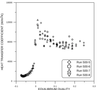
Run 500-5 Run 500-6 Run 500-7 Run 500-8
Figure 5. High inlet subcooling experimental runs (500 mbar exit pressure).
-0.1 0 0.1 0.2 0.3
EQUILIBRIUM QUALITY
0 2000 4000 6000 8000 10000
H
E
A
T
T
R
A
N
S
F
E
R
C
O
E
F
F
IC
IE
N
T
(
W
/m
2K
)
Run 1000-5 Run 1000-6 Run 1000-7 Run 1000-8
Figure 6. High inlet subcooling experimental runs (1000 mbar exit pressure).
Discussions
Following from a series of deductions and elimination of clues offered by the trends and experimental observations noted during these experimental runs, it is postulated that the most probable explanation of this intriguing phenomenon is the existence of localized thermal non-equilibrium instability as proposed and described by Jeglic and Grace (1965), and elaborated by Ishii (1982).
As stated in previous introductory section, Jeglic and Grace (1965) found that, for flow oscillations to occur, the rate of change in void fraction has to be high and abrupt subcooled flow boiling. Ishii (1982) extended on this postulation by stating that from the operating conditions Jeglic and Grace had employed, and because of poor nucleation and heat transfer, the liquid can become highly superheated. However, once a bubble is nucleated, it grows explosively due to the high liquid superheat. The consequences of this explosive like growth are a very rapid increase in void fraction, a sudden release of thermal energy stored in the superheated liquid into the bubble growth and the removal of heat from the wall,
causing a drop in wall temperature. Compounded together, these effects will cause the sudden rise in the value of heat transfer coefficient as shown in Figs. 4 to 6.
It should be noted here that one may argue that a drop in wall temperature is to be expected in all flow boiling experiments at the inception of nucleate boiling. However, in the present study, the key difference is that because of the higher specific volume of steam at low pressures, a given amount of heat released from the superheated liquid and the wall would create a much larger volume of vapour.
Although the findings of Jeglic and Grace (1965) cannot be quantitatively linked to the experimental results reported here, one can relate them through the following points and trends:
1. The heat transfer coefficient maxima at low qualities were found to be dependent of inlet subcooling. Its value is lower at low inlet subcooling. Jeglic and Grace (1965) argued that in their experimental results, when the inlet subcooling is small, the heat flux required for net vapour generation is lower than that for larger subcooling. Consequently, the rate of change of void fraction was expected to be less, resulting in a smoother transition from bubbly to annular flow. They suggest that for flow oscillations to occur, the transition must be abrupt, so that high inlet subcooling makes the system more susceptible to the instability. In the present experiments, however, the inlet subcooling is changed independently of heat flux. A possible explanation of the influence of subcooling is that, with low subcooling, nucleate boiling at the wall is initiated early in the test section and thus, prevents excessive superheats in the liquid. At higher inlet subcoolings, on the other hand, nucleate boiling does not occur immediately and its eventual occurrence may be associated with the instability phenomenon described above.
2. The heat transfer coefficient maxima were found to be dependent on exit pressure (i.e., system pressure). The higher the system pressure, the lower the value of heat transfer coefficient. In their study, Jeglic and Grace (1965) argued that for higher pressure systems, flow oscillations could not be obtained in the subcooled boiling region. They argued that the decrease in latent heat of vaporization with increasing pressure is much less than the corresponding decrease in liquid-vapour density ratio, see Tab. 2. Thus, according to them, the net effect of pressure increase would be a lower rate of change of void fraction, which in their studies, is unfavorable for flow oscillations, while the same arguments applied here would imply that the rapid heat removal associated with the rapid vaporization and void growth is reduced.
3. As can be seen from Tab. 2, the tendency for the liquid to superheat is much greater as the pressure decreases, since the latent heat of vaporization rises while the liquid thermal conductivity decreases. Both factors may account for a less efficient single-phase heat transfer across the liquid layer next to the heated wall into the bulk fluid core, resulting in a more superheated layer of liquid. This effect may explain the existence (even at high pressures) of the heat transfer coefficient maximum in freon refrigerant and hydrocarbon systems as reported by Thome (1995), Kandlbinder (1997) and Urso et al. (2002). The thermal conductivity of refrigerants and hydrocarbons is much less than that of water. The physical properties of typical refrigerants and light hydrocarbons are given in Tab. 3.
greater at lower pressures. Small pressure fluctuations were also observed and both these observations support the hypothesis (consistent with the suggestion of Jeglic and Grace, 1965) that localized thermally induced instabilities may have been taking place.
Table 2. Some key saturated water/steam physical properties at different pressures (extracted from REFPROP v. 7.0, Lemmon et al., 2002).
p
(mbara)
L ρ
(kg/m3)
G ρ
(kg/m3)
G L ρ ρ (-) v h ∆ (kJ/kg) L λ (W/m.K)
250 980.5 0.16 6082.3 2345.4 0.659
500 970.9 0.31 3145.9 2304.6 0.671
1000 958.6 0.59 1623.9 2257.4 0.679
Table 3. Some key saturated physical properties of selected refrigerants at 1000 mbara. (extracted from REFPROP v. 7.0, Lemmon et al., 2002).
Substance ρL (kg/m3)
G ρ
(kg/m3)
G L ρ ρ (-) v h ∆ (kJ/kg) L λ (W/m.K)
Isobutane 594.2 2.79 212.8 366.25 0.103
n-Pentane 610.2 3.00 203.4 358.20 0.107
R-134a 1377.5 5.19 265.3 217.16 0.104
R-141b 1221.0 4.79 254.7 223.09 0.089
Based on the observations presented above, the existence of localized thermally induced instabilities seems to be an explanation for the heat transfer coefficient maxima at high inlet subcoolings, low vapour qualities and low pressures as noted in the SAE experiments. It is noteworthy that visual manifestations of the instability were not observed in the viewing section at the end of the test section. However, the heat transfer coefficient maxima happened within the first 1 m (44 diameters) of the test section, and with another 3 m (130 diameters) of heated test section to go, any small flow instability may have been damped out as the flow moves into the churn and annular flow regimes as observed in the visualization section.
Modelling
Summary of the Model
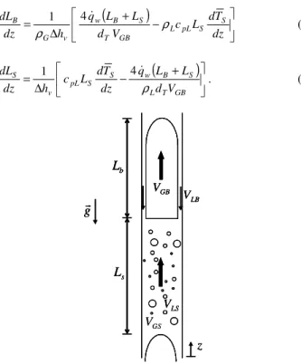
The non-equilibrium slug flow model (NESM) is described in full in Barbosa and Hewitt (2005) and only its main features will be described here. Its fundamental structure is a slug unit consisting of a Taylor bubble surrounded by a falling liquid film and a liquid slug, as seen in Fig. 7.
It is assumed that when the conditions are such that abrupt vapour growth takes place in the subcooled region (see Experimental Analysis), large Taylor bubbles are generated. As they are formed, the Taylor bubbles become separated by regions of subcooled liquid (subcooled slugs). The falling film surrounding the Taylor bubble is assumed saturated, i.e., a considerable portion of the energy associated with the high wall temperatures in the near-wall region is used up during the process of generation of the Taylor bubble. Phase change and gas hold-up within the liquid slug are assumed negligible. It is further hypothesized that the thickness of the liquid film surrounding the Taylor bubble is small compared with the pipe diameter, the mass of the liquid film is small compared with that of the slug, the densities do not vary strongly with time/distance and VGB>>dLB dt , then dt dz=1VGB. An energy balance over the slug unit gives (Barbosa and Hewitt, 2005)
(
)
− + ∆ = dz T d L c V d L L q h dz dL S S pL L GB T S B w v G B ρ ρ 4 1 (2)(
)
+ − ∆ = GB T L S B w S S pL v S V d L L q dz T d L c h dz dL ρ 4 1. (3)
b L s L GB V LB V LS V g z GS V b L s L GB V LB V LS V g z b L s L GB V LB V LS V g z GS V
Figure 7. A schematic representation of slug flow.
An energy balance within the liquid slug gives the average slug temperature variation as follows
(
sat S)
B S L G LS pL L w T S T T dz dL L V c q d dz T d − −
= 4 ρ ρρ 1 . (4)
In the thermal non-equilibrium region, i.e. TS
( )
z <Tsat, the liquid slug temperature gradient, the Taylor bubble growth rate and the liquid slug contraction rate are given by the simultaneous solution of Eqs. (2)-(4). A stepwise numerical integration of this system of equations gives local values of LB, LSand TSalong the thermal non-equilibrium slug region. The thermal non-equilibrium slug region is bounded by the onset of slug flow (calculated with the correlation of Saha and Zuber (1974) for the Point of Net Vapor Generation, NVG, and by the transition to saturated slug flow or by the break-up of non-equilibrium slug flow into churn flow, whichever happens first ― see flow chart in Fig. 8 below).Calculation of additional slug flow parameters such as the Taylor bubble length fraction, β, and the real quality (vapour mass fraction), xG , as well as the determination of boundary conditions for Eqs. (2)-(4) are performed exactly as in Barbosa and Hewitt (2005). In the slug flow regime, the time averaged wall temperature is given by (disregarding the thermal capacity of the heated wall),
(
)
(
)
wSf w S w ss f w sf sp t t t w t w sp w T T T t T t t dt T dt T t T ss sf sf sf , , , , 0 1 1 1 β
β + −
where the time averaged wall temperatures in the slug and falling film regions are determined using heat transfer superposition models (Chen, 1966) as follows,
(
wS S)
nbS(
wS sat)
S fc
w T T T T
q =α , , − +α , , − (6)
(
fcf nbf)(
wf sat)
w T T
q =α , +α , , − (7)
where the various heat transfer coefficients (for the nucleate boiling and forced convective mechanisms) are given by the correlations reported in Barbosa and Hewitt (2005).
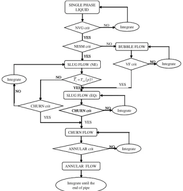
In addition to the slug flow heat transfer calculation, a methodology to compute the pressure drop along the channel was implemented. The methodology encompasses all flow regimes, from single-phase subcooled liquid to saturated annular flow. The various models for each flow pattern and criteria for the transitions between flow patterns are summarized in Fig. 8 and Tab. 4. The first transition criterion is the NVG correlation of Saha and Zuber (1974), implemented as described by Barbosa and Hewitt (2005). The non-equilibrium slug flow transition criterion (NESM criterion) yields two possible outcomes; in the first, flow conditions are such that non-equilibrium slug flow does not take place and there is a more usual succession of flow patterns (bubble, slug, churn and annular flow). The second outcome is associated with the transition to non-equilibrium slug flow and is expected to take place in sub-atmospheric boiling of water at high inlet subcoolings and in boiling of pure hydrocarbons (Kandlbinder, 1997). The transition from non-equilibrium to non-equilibrium slug flow is associated with the attainment of saturation in the liquid slug and the transition from non-equilibrium slug flow to churn flow is associated with the occurrence of flooding in the Taylor bubble region (Jayanti and Hewitt, 1992). Integration of the governing equations (mass, momentum and energy) is performed using a 4th order Runge-Kutta Method (Press et al., 1992).
SINGLE PHASE LIQUID
YES
NO Integrate
SLUG FLOW (NE)
BUBBLE FLOW NVG crit
NESM crit NO
YES
VF crit
( )p T Ts=sat
SLUG FLOW (EQ) ? NO
NO Integrate
YES YES
CHURN crit Integrate
NO
CHURN FLOW
CHURN crit NO
Integrate
YES YES
ANNULAR crit NO Integrate
ANNULAR FLOW
Integrate until the end of pipe SINGLE PHASE
LIQUID
YES
NO Integrate
SLUG FLOW (NE)
BUBBLE FLOW NVG crit
NESM crit NO
YES
VF crit
( )p T Ts=sat
SLUG FLOW (EQ) ? NO
NO Integrate
YES YES
CHURN crit Integrate
NO
CHURN FLOW
CHURN crit NO
Integrate
YES YES
ANNULAR crit NO Integrate
ANNULAR FLOW
Integrate until the end of pipe
Figure 8. A flow diagram of the two-phase flow calculations.
Table 4. Summary of the two-phase flow models utilized in the present study.
Flow regime
Transition criterion
Fric. pressure gradient
Void fraction Single-phase
liquid flow
―
Colebrook friction factor
(Potter and Wiggert, 2002)
―
Bubble
flow εG =0.25
Friedel (1979)
Zuber and Findlay (cf. Collier and
Thome, 1994)
Thermal Non-Equilibrium Slug flow
NVG Point associated with
explosive like bubble growth (Saha and Zuber, 1974)
De Cachard and Delhaye (1996)
De Cachard and Delhaye
(1996)
Thermal Equilibrium
Slug flow
:
( )
p T TS = satDe Cachard and Delhaye (1996)
De Cachard and Delhaye
(1996)
Churn flow
Jayanti and Hewitt (1992)
model
Sawai et al.
(2004)
Sawai et al.
(2004)
Annular flow
Wallis (1969) model
Hewitt and Whalley (1978) interfacial friction
factor.
Triangular relationship between film thickness, film
flow rate and pressure drop (Govan, 1990)
Results
Figures 9 to 11 illustrate the local heat transfer coefficient profiles as a function of quality together with curves indicating the difference between the equilibrium bulk temperature and the liquid slug temperature in the region between the NVG Point and the transition to churn flow (breakdown of slug flow), as calculated by the non-equilibrium slug flow model. The temperature difference increases sharply from zero up to a few degrees in all three cases and then decreases in the equilibrium saturated region (xeq>0), Curves of equilibrium quality as a function of distance are also shown. As observed in boiling of hydrocarbons (Barbosa and Hewitt, 2005), the temperature difference peaks coincide with those for the heat transfer coefficient in Figs. 9 and 10 (sub-atmospheric pressures). This is consistent with the observations of Jeglic and Grace (1965) in that once the large nucleated bubble fills the pipe cross-section, it continues to grow, increasing the fluid velocity and reducing the residence time in the channel of the liquid slugs between successive bubbles. Thus, slugs remain subcooled for distances longer than would be the case for equilibrium flow conditions. A consequence of this effect is that the wall temperature in the slug flow region is lower than that in the equilibrium case. As the heat transfer coefficient is defined in terms of an equilibrium relationship, the net result is an increase in the heat transfer coefficient. Figures 9 and 10 show that the decrease of the heat transfer coefficient back towards the classical behavior of forced convective boiling (i.e., absence of peaks) corresponds to the region of breakdown of slug flow into churn flow (S/C). Since this transition is related to the collapse of the slug unit, the mixing of the phases would result in attainment of thermodynamic equilibrium, thus eliminating remaining local subcooling effects.
with the Chen correlation (Chen, 1966; Butterworth and Shock, 1982). The NESM predictions are consistently higher than those provided by the Chen correlation in the slug flow region. For the lowest pressure case (250 mbar abs.) of Fig. 9, the NESM is not capable of predicting the exceedingly high peaks of nearly 20 kWm
-2
K-1. The predictions are, however, much more encouraging at intermediate pressures (500 mbar abs.) where the model performance is within a few percent of the experimental values (see Fig. 10).
-0.1 0 0.1 0.2 0.3
EQUILIBRIUM QUALITY 0 10000 20000 H E A T T R A N S F E R C O E F F IC IE N T ( W m -2K -1) 0 2 4 6 8 D IS T A N C E ( m ); T E M P E R A T U R E D IF F E R E N C E ( OC )
Heat transfer coefficient Distance
TBULK-TSLUG
Present work (NESM) Chen (1966)
S/C NVG
Figure 9. Difference between the equilibrium and slug temperatures as a function of distance. Comparison between experimental and calculated heat transfer coefficients in the region between the NVG Point and the Slug-to-Churn flow transition. Run 250-5.
-0.1 0 0.1 0.2 0.3
EQUILIBRIUM QUALITY 0 4000 8000 12000 H E A T T R A N S F E R C O E F F IC IE N T ( W m -2K -1) 0 2 4 6 8 D IS T A N C E ( m ); T E M P E R A T U R E D IF F E R E N C E ( OC )
Heat transfer coefficient Distance TBULK-TSLUG
Chen (1966) Present work (NESM) S/C
NVG
Figure 10. Difference between the equilibrium and slug temperatures as a function of distance. Comparison between experimental and calculated heat transfer coefficients in the region between the NVG point and the Slug-to-Churn flow transition. Run 500-6.
In Fig. 11, there are no distinct heat transfer peaks in the near-zero quality region. Since the exit pressure is nearly atmospheric, non-equilibrium slug flow is not expected to occur. Nevertheless, the NESM predictions are shown for the sake of comparison with the equilibrium formulation. In this case, despite somewhat under predicted, the heat transfer coefficient is better correlated by the Chen (1966) model. The trends of the heat transfer coefficient
predictions depicted in Figs. 9 to 11 are representative of all experimental runs conducted in the present work.
-0.1 0 0.1 0.2 0.3
EQUILIBRIUM QUALITY 0 4000 8000 12000 H E A T T R A N S F E R C O E F F IC IE N T ( W m -2K -1) 0 2 4 6 8 D IS T A N C E ( m ); T E M P E R A T U R E D IF F E R E N C E ( OC )
Heat transfer coefficient Distance
TBULK-TSLUG
Chen (1966) Present work (NESM)
NVG S/C
Figure 11. Difference between the equilibrium and slug temperatures as a function of distance. Comparison between experimental and calculated heat transfer coefficients in the region between the NVG Point and the Slug-to-Churn flow transition. Run 1000-5.
Figure 12 shows an overall comparison of heat transfer coefficients in the non-equilibrium slug flow region for the 250 mbar and 500 mbar runs. Although the NESM predictions show some improvement over existing equilibrium models (for example, the Chen correlation), the model does not predict the very high heat transfer peaks associated with the 250 mbar (250-7A and 250-7B) runs (under predictions lower than -40%). The six experimental data points over predicted by more than 40% correspond to the 250-1 and 250-3 runs; those in which no heat transfer peaks were observed and for which the inlet subcoolings were low.
0 10000 20000 30000 40000
EXPERIMENTAL HEAT TRANSFER COEFFICIENT (Wm-2K-1)
0 4000 8000 12000 C A L C U L A T E D H E A T T R A N S F E R C O E F F IC IE N T ( W m -2K -1)
Present model (NESM) Chen (1966)
-40% +40%
Figure 12. Comparison of local heat transfer predictions for the sub-atmospheric pressure runs (Runs 250-1, 6, 7A, 8A, 7B and 8B and Runs 500-5, 6, 7 and 8).
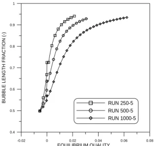
Taylor bubble growth rate is higher for the lower pressure as a result of the larger liquid-vapour density ratio.
-0.02 0 0.02 0.04 0.06 0.08
EQUILIBRIUM QUALITY
0.4 0.5 0.6 0.7 0.8 0.9 1
B
U
B
B
L
E
L
E
N
G
T
H
F
R
A
C
T
IO
N
(
-)
RUN 250-5 RUN 500-5 RUN 1000-5
Figure 13. Variation of bubble length fraction as a function of equilibrium quality typical sub-atmospheric pressure runs.
Figure 14 shows the overall pressure gradient predictions using the present model. The run number is shown together with the symbol. As can be seen, the majority of the predictions lie within ± 12.5% of the experimental values, reflecting the capability of the methodology in predicting the pressure drop data.
3000 4000 5000
EXPERIMENTAL PRESSURE GRADIENT (Nm-3)
3000 4000 5000
C
A
L
C
U
L
A
T
E
D
P
R
E
S
S
U
R
E
G
R
A
D
IE
N
T
(
N
m
-3)
250-1 250-3
250-5 250-6
250-7A
250-7B 250-8B
500-5 500-6
500-7
1000-5 1000-7
-12.5% +12.5%
Figure 14. Average pressure gradient predictions.
Conclusions
The following conclusions were drawn from the experimental and modelling studies carried out in the present paper:
1. The experiments were found to be nucleate boiling dominant for thermodynamic qualities less than 0.05; 2. Heat transfer coefficient maxima were observed at around
zero thermodynamic quality for the results at high liquid inlet subcoolings and low sub-atmospheric pressures. The localized thermal non-equilibrium instability hypothesis presented by Jeglic and Grace (1965) provided a possible explanation;
3. The system pressure and inlet subcoolings were shown to influence flow stability in accordance with the Jeglic and Grace (1965) hypothesis. However, it should be noted that the instrumentation used here were not specifically designed to investigate these unusual effects. They were observed and noted as having occurred during a program of study on the axial heat transfer coefficient variation of flow boiling at sub-atmospheric pressures. Consequently, it is recommended that further external and independent investigations be carried out to confirm the above mentioned effects.
4. It was shown that the heat transfer peaks agree with the liquid slug equilibrium sub-cooling peaks and higher heat transfer coefficients are predicted by the proposed modelling approach in the near zero equilibrium quality region. Although not particularly accurate (±40% error band), the model predictions are better than those given by an equilibrium formulation in cases where the occurrence of thermal non-equilibrium instabilities is expected. 5. In addition to the heat transfer coefficient comparison,
overall pressure gradients were predicted for a number of conditions as part of the two-phase flow calculation methodology and these were shown to be in very good agreement with the experimental data.
References
Barbosa, Jr., J.R. and Hewitt, G.F., 2005, “A thermal non-equilibrium slug flow model”, J. Heat Transfer, Vol. 127, No. 3, pp. 323-331.
Butterworth, D. andShock, R.A.W., 1982, “Flow boiling”, Proceedings of the 7th International Heat Transfer Conference, Vol. 1, Munich, Germany, pp. 11-30.
Carey, V.P., 1992, “Liquid-Vapor Phase Change Phenomena”, Hemisphere Publishing Co, Washington DC, 645 p.
Cheah, L.W., 1996, “Forced convective evaporation at sub-atmospheric pressure”, Ph.D. Thesis, Imperial College, London.
Chen, J.C., 1966, “A correlation for boiling heat transfer to saturated fluids in convective flow”. Ind. Eng. Chem.: Proc. Des. Develop., Vol. 5, No. 3, pp. 322-329.
Collier, J.G. and Thome, J.R., 1994, “Convective Boiling and Condensation”, Oxford University Press, 596 p.
De Cachard, F. and Delhaye, J.M., 1996, “A slug-churn flow model for small-diameter airlift pumps”, Int. J. Multiphase Flow, Vol. 22, No. 4, pp. 627-649.
Friedel, L., 1979, “Improved friction pressure drop correlations for horizontal and vertical two-phase pipe flow”, European Two-Phase Flow Group Meeting, Ispra, Italy, paper E2.
Govan, A.H., 1990, “Modelling of vertical annular and dispersed two-phase flow”, Ph.D. Thesis, Imperial College, London.
Hewitt, G.F. and Whalley, P.B., 1978, “The correlation of liquid entrained fraction and entrainment rate in annular two-phase flow”, UKAEA Technical Report AERE-9187.
Hewitt, G.F., 2001, “Deviations from classical behaviour in vertical channel convective boiling”, Multiphase Science and Technology, Vol. 13, No.3-4, pp. 161-190.
Ishii, M., 1982, “Wave Phenomena and Two-Phase Flow Instabilities”. In: Handbook of Multiphase Systems (Ed. G. Hetsroni), Hemisphere Publishing Co, Washington DC.
Jayanti, S. and Hewitt, G.F., 1992, “Prediction of the slug-to-churn transition in vertical two-phase flow”, Int. J. Multiphase Flow, Vol. 18, No. 6, pp. 847-860.
Jeglic, F.A. and Grace, T.M., 1965, “Onset of flow oscillations in forced flow subcooled boiiling”. NASA Technical Note TN D-2821, Lewis Research Center, Cleveland, Ohio, USA.
Kandlbinder, T.K., 1997, “Experimental investigation of forced convective boiling of hydrocarbons and hydrocarbon mixtures”, Ph. D. Thesis, Imperial College, London.
Kattan, N., Thome, J.R. and Favrat, D., 1995, “Development of boiling heat transfer and its applications”, 2nd International Conference on
Lemmon, E.L., McLinden, M.O., Huber, M.L.; 2002, “REFPROP 7.0 – Reference Fluid Thermodynamic and Transport Properties”, NIST, Boulder, CO.
Potter, M.C., Wiggert, D.C., Hondzo, M. and Shih, T.I.P., 2002, “Mechanics of Fluids”, 3rd Edition, Prentice-Hall.
Press, W.H., Teukolsky, S.A., Vetterling, W.T. and Flannery, B.P., 1992, “Numerical Recipes in FORTRAN – The Art of Scientic Computing”, Cambridge University Press, 2nd Edition.
Saha, P. & Zuber, N., 1974, “Point of net vapor generation and vapor void fraction in subcooled boiling”, 5th International Heat Transfer Conference, Tokyo, Japan, paper B4.7.
Sawai, T., Kaji, M., Kasugai, T., Nakashima, H. and Mori, T., 2004, “Gas–liquid interfacial structure and pressure drop characteristics of churn flow”, Exp. Therm. Fluid Sci., Vol. 28, No. 6, pp. 597-606.
Spindler, K., 1994, “Flow boiling”, 10th International Heat Transfer
Conference, Vol. 1, Brighton, UK, pp. 349-368.
Stone, J.R., 1971, “Subcooled and net boiling heat transfer to low-pressure water in electrically heated tubes” NASA Technical Note TN D-6402, Lewis Research Center, Cleveland, OH.
Thome, J.R., 1995, “Flow boiling in horizontal tubes: a critical assessment of current methodologies”, 1st Symposium on Two-Phase Flow
Modelling and Experimentation Conference, Vol. 1., 41-52.
Urso, M.E., Wadekar, V.V. and Hewitt, G.F., 2002, “Flow boiling at low mass flux”, 12th International Heat Transfer Conference, Grenoble, France, pp. 803-808.