746 Brazilian Journal of Physics, vol. 36, no. 3A, September, 2006
A New Method to Study Stochastic Growth Equations: Application
to the Edwards-Wilkinson Equation
T. G. Mattos, J. G. Moreira, and A. P. F. Atman Departamento de F´ısica, Instituto de Ciˆencias Exatas,
Universidade Federal de Minas Gerais, C.P. 702 30161-123, Belo Horizonte, MG - Brazil
Received on 30 September, 2005
In this work we introduce a method to study stochastic growth equations, which follows a dynamics based on cellular automata modeling. The method defines an interface growth process that depends on height differences between neighbors. The growth rules assign a probability pi(t)for siteito receive a particle at timet, where pi(t) =ρexp[κΓi(t)]. Hereρandκare two parameters andΓi(t)is a kernel that depends on heighthi(t)of site iand on heights of its neighbors, at timet. We specify the functional form of this kernel by the discretization of the deterministic part of the equation that describes some growth process. In particular, we study the Edwards-Wilkinson (EW) equation which describes growth processes where surface relaxation plays a major role. In this case we have a Laplacian term dominating in the growth equation andΓi(t) =hi+1(t) +hi−1(t)−2hi(t), which follows from the discretization of∇2h. By means of simulations and statistical analysis of the height
distributions of the profiles, we obtain the roughening exponents,β, αandz, whose values confirm that the processes defined by the method are indeed in the universality class of the original growth equation.
Keywords: Cellular Automata; Interface Growth; Dynamic Scaling
I. INTRODUCTION
In nature, as well as in physics laboratories and industrial applications, one can find a large sort of rough surfaces (or interfaces) and the interest in studying such structures has in-creased in the last decades[1–3]. In a computational approach, one can develop discrete growth models based on a set of sym-metries and conservation laws. Proceeding with simulations, one can obtain the scaling exponents and other quantities of interest.
On the other hand, one can write stochastic (continuum) growth equations in order to give an analytical approach to the problem of interface growth, obeying the same symme-tries and conservation laws considered in the definition of the mentioned discrete models. Obviously, the agreement of re-sults from both points of view, discrete and continuous, is of fundamental importance.
In the study of interface growth dynamics, one is mostly concerned about the temporal behavior of the interface rough-ness, which is a measure of the interface width. The most relevant information about the dynamical details of a growth process can be obtained from the temporal behavior of the roughness. In particular, for self-affine interfaces, it is known that the roughness grows with time as a power law, where we define thegrowth exponent,β. Actually, due to correlations, the roughness does not grow indefinitely with time; the inter-face eventually reaches a stationary regime where the rough-ness saturates. Both the saturation roughrough-ness and saturation time depend on the system size as a power law, for which we define theroughness exponent,α, and thedynamic exponent, z, respectively.
A set of values for these three roughening exponents, in a given dimension, defines an universality class. Thus, if two or more processes have the same exponents values, one can say that they belong to the same universality class, which means that their underlying dynamics obey the same symmetries and
conservation laws.
In this work we introduce a method[4] to study sto-chastic differential equations that describe interface growth processes. This method is based on a cellular automata dynamics[5], in a sense that we associate a particle deposition probability to each site, which depends on the local height profile, considering a synchronous update scheme. Other works that apply cellular automata models to study growth processes have also been done lately[6–8].
Our goal is to show that the method introduced provides the expected results for the universality class of the equation that we are interested in studying. In this paper we apply this method to the Edwards-Wilkinson (EW) equation, which is associated to the random deposition with surface relaxation. In section II we introduce the basic concepts and relevant quantities in the study of interface growth phenomena. In sec-tion III we introduce the method and discuss its main features. In section IV we present the simulations results obtained by the application of the method to the EW equation, showing that the method introduced indeed reproduces the expected results for this universality class. Finally, we draw some con-clusions and perspectives in section V.
II. DEFINITIONS
The discrete computational growth models we are consid-ering in this paper are defined in a one-dimensional lattice of size L, initially flat and with periodic boundary conditions. The deposition processes occur in discrete time steps and, in general, we define one time step as the deposition ofL parti-cles. The particles are all identical.
T. G. Mattos et al. 747
ω2(L,t) = 1
L
L
∑
i=1
£
hi(t)−h(L,t)¤
2
, (1)
where
h(L,t) =1
L
L
∑
i=1
hi(t) (2)
is the mean height of the interface.
The roughness provides a measure of the interface width and generally, in growth processes, we have a power law for its temporal behavior,
ω∼tβ, (3)
whereβis the growth exponent. For the simplest deposition model, the random deposition (RD), it is known[2] that the roughness grows indefinitely, withβ=1/2. The main char-acteristic of the RD model is that no correlations are present in the dynamics, hence the collums grow independently from each other.
For other deposition models, where there are correlations among the sites, it is known[2] that the roughness grows ini-tially as the power law (3) and then stabilizes in a value, the saturation roughnessωsat, after a saturation timetx, for which
we have
ωsat∼Lα, (4)
tx∼Lz, (5)
whereαis the roughness exponent andzis the dynamic expo-nent. The three exponents are not independent and, using the Family-Vicsek scaling law[9], it is possible to collapse curves
ω xt obtained for various system sizes onto a single curve f(u), called scaling function.
Consider for example the random deposition with surface relaxation model (RDSR)[10]. The particle is deposited in a random position in the lattice and is allowed to relax to the position of lowest height, considering the first neighbors. In this way, the particle flux is larger for local minimum than for local maximum positions. For this model the exponent values, ind=1, are[2, 10]
α=1
2 , β= 1
4 , z= 2.
In order to provide an analytical approach to the study of interface growth, one can construct a stochastic growth equa-tion based on the discrete model. However, there is no direct way to derive an equation from the discrete model. All one can do is write down an equation that respects the same sym-metries of the discrete model[2] and hope for the best. If the
analytical solutions match the previous results obtained from the simulations, one can say that the given equation can be correctly associated to the discrete model.
As we have seen, the particle flux in the RDSR model is larger for local minimum positions. So it is reasonable to say that the time derivative of the local height profile is propor-tional to the Laplacian. Thus, in order to associate a stochastic equation to this deposition model, we write
∂h(x,t)
∂t = ν∇
2h(x,t) +η(x,t), (6)
where in the left hand side we have the temporal variation of the height at position x, while in the right hand side we haveν>0 and η(x,t), which is a white noise (zero aver-age, δ-correlated in space and time). This is the Edwards-Wilkinson equation[11], or simply EW equation, which pro-vides the same exponent values obtained for the RDSR model and hence can be correctly associated to this model.
III. THE METHOD
Consider a one-dimensional lattice of sizeL, initially flat and with periodic boundary conditions. Each time step, all the sites aresimultaneouslyvisited so that siteireceives a particle at timetwith probabilitypi(t)given by
pi(t) =ρeκΓi(t). (7)
Here 0<ρ<1 andκ>0 are two parameters, fixed through-out the evolution of the interface, andΓi(t)is a kernel that
de-pends on the heights of siteiand its neighbors. The particular functional form ofΓi(t)will be given by the discretization of
the deterministic part of the growth equation we are intended to study. In the case of the EW equation (6), the kernel is given by the discretization of the Laplacian∇2h,
Γi(t) =hi+1(t) +hi−1(t)−2hi(t). (8)
In the way we have defined the method, we can eventually get pi(t)>1. In this situation, we impose the condition
pi(t)≥1 =⇒ pi(t) =1 =⇒ hi(t+1) =hi(t) +1 .
IV. SIMULATIONS RESULTS
748 Brazilian Journal of Physics, vol. 36, no. 3A, September, 2006
make sure of the value of the growth exponent, we show in the inset the roughness divided byt1/4as a function oft, for the same values of the parametersρandκ, but for larger systems (L=102, 103and 104). In this case, a horizontal line means
β=1/4 and as one can see, the larger the system size, the closer to 1/4 is the value of the growth exponent, and longer the system stays in this regime.
0 50 100 150 200 250 300 350 400 450 500 i
0 100 200 300 400
h
100 101 102 103 104 105 106
t
100
ω
t
ω / t1/4
y = x1/4
FIG. 1: In the top we show a typical profile forρ=0.5,κ=0.1 and L=500, where we change the color of the particles each 50 time steps and let the system evolve untilt=750. In the bottom, we have a log-log plot of the roughnessωas a function of timet, forρ=0.5,κ=0.1 andL=200, averaged over 200 samples. The traced line corresponds to the functiony=x1/4. In the inset we show the roughness divided byt1/4as a function oft, forL=102, 103and 104.
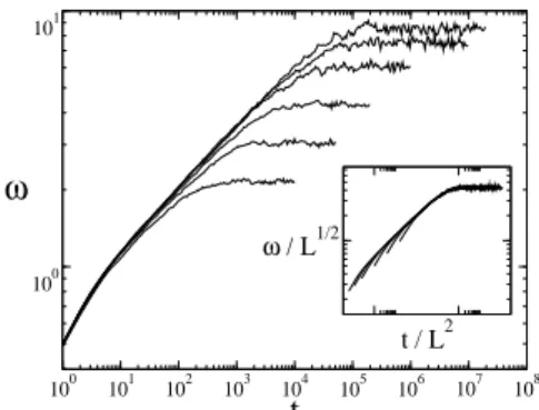
In order to obtain the values of the roughness and dynamic exponents, α and z, we let the system reach the saturation regime for some system sizes, betweenL=25 andL=400, still keepingρ=0.5 andκ=0.1, as one can see in figure 2. In the inset, we show that a good collapse, withα=1/2 and z=2, was obtained, confirming thus that the method, with the kernel given in equation (8), is indeed in the EW universality class.
We then proceed by showing the results obtained by varying the parameter κ. As one can see in the left of figure 3, we identified aκ-dependent crossover between the RD and the RDSR regimes. Initially we haveβ=1/2 and thenβ=1/4 and the crossover timetcincreases asκdecreases. In fact we
found a power law fortcas function ofκ,
tc∼κz
′
κ, (9)
withz′κ=−1.02(2), as one can see in the right of figure 3. Thus, for smallκ, the system will stay more time in a RD regime with deposition rateρ. In fact, the lower the value ofκ, the higher the value ofΓi(t)must be so thatpi(t)6=ρ, which
100 101 102 103 104 105 106 107 108
t
100 101
ω
t / L2
ω / L1/2
FIG. 2: Keepingρ=0.5 andκ=0.1, we varied the system size and plotted the roughnessωagainst timet, forL=25,50,100,200,300 and 400 - from bottom to top. In the inset we show the good collapse obtained withα=1/2 andz=2. These graphics are in a log-log scale.
100 101 102 103 104 105
106
107 108
t
100
101
102
ω
10-6
10-5
10-4 10-3 10-2 κ
102
104 106
tc
κ = 0.001
κ = 0.01
κ = 0.1 y ~ x1/2
y ~ x1/4
t
c~
κ
−1.02(2)FIG. 3: In the left we have log-log plot of the roughnessω as a function of timetforL=250,ρ=0.5 andκ=10−3,10−2and 10−1. This result is averaged over 40 samples. Initially we haveβ=1/2 and thenβ=1/4, as one can see by comparing with the traced and dotted lines, respectively. In the right, we show the crossover timetc as a function ofκ, forL=250 andρ=0.5. Forκ>0.02 it is hard to get precise values fortc.
means that the interface roughness must be large enough so that correlations can be seen in the system.
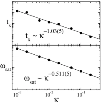
We also studied the dependence of the saturation roughness and saturation time,ωsatandtx, with the parameterκand we
found that
tx∼κzκ, (10)
ωsat∼κακ, (11)
withακ=−0.511(5) and zκ=−1.03(5), as one can see in
figure 4.
V. CONCLUSIONS AND PERSPECTIVES
T. G. Mattos et al. 749
tx
10-3 10-2 10-1
κ
ωsat
t
x~
κ
−1.03(5)ω
sat~
κ
−0.511(5)FIG. 4: Log-log plot of the saturation roughness and saturation time, ωsatandtx, as functions of the parameterκ. Hereρ=0.5,L=250;
the results are averaged over 25 samples. The straight lines are linear fits to the data.
proving that the method was successful in this application. We also found a crossover between the RD and RDSR classes when we varied the parameterκ. A power law behavior was found for the crossover timetc, the saturation roughnessωsat
and the saturation timetx, as functions ofκ. As perspectives
we are intended to apply this method in the study of other equations such as the Kardar-Parisi-Zhang equation[12] and the equation of growth with surface diffusion[13, 14]. We shall also apply this method to growth in two-dimensional substrates.
Acknowledgments
We thank R. Dickman for helpful criticism of the manu-script. This work is supported by Brazilian agency CNPq.
[1] F. Family and T. Vicsek,Dynamics of Fractal Surfaces, World Scientific, Singapore (1991)
[2] A.-L. Barab´asi and H.E. Stanley,Fractal Concepts in Surface Growth, Cambridge Univ. Press, Cambridge (1995)
[3] P. Meakin,Fractals, scaling and growth far from equilibrium, Cambridge Univ. Press, Cambridge (1998)
[4] T.G. Mattos, “Autˆomatos celulares e crescimento de interfaces rugosas”, Master thesys, UFMG (2005)
[5] S. Wolfram, Theory and Applications of Cellular Automata, World Scientific, Singapore (1986) ; Rev.Mod.Phys.55, 3, 601 (1983)
[6] A.P.F. Atman, R. Dickman, and J.G. Moreira, Phys.Rev.E66, 016113 (2002)
[7] A.P.F. Atman and J.G. Moreira, Eur.Phys.J. B 16 (3), 501 (2000)
[8] T.G. Mattos and J.G. Moreira, Brazilian Journal of Physics,34, 448 (2004)
[9] F. Family and T. Vicsek, J.Phys. A18, L75-L81 (1985) [10] F. Family, J.Phys. A19, L441 (1986)
[11] S.F. Edwards and D.R. Wilkinson, Proc.R.Soc.Lond. A381, 17-31 (1982)
[12] M. Kardar, G. Parisi, and Y.C. Zhang, Phys.Rev.Lett.56, 889 (1986)