0103 - 5053 $6.00+0.00
Article
*e-mail: [email protected]
Gaseous and Particulate Atmospheric Mercury Concentrations in the Campinas Metropolitan
Region (São Paulo State, Brazil)
Anne H. Fostier* and Paula A.M. Michelazzo
Instituto de Química, Universidade Estadual de Campinas, CP 6154, 13082-864 Campinas-SP, Brazil
As concentrações de Mercúrio Gasoso Total (MGT) e Mercúrio Particulado Total (MPT) foram monitoradas durante as estações seca e úmida de 2002-2003 em dois pontos (industrial e residencial) da Região Metropolitana de Campinas. Não foi observada diferença significativa entre as concentrações dos pontos de amostragem e as concentrações médias foram 7,0 ± 5,8 ng m-3 (MGT) e 0,4 ± 0,3 ng m-3 (MPT). A análise da variação nictemeral mostrou maior
concentração de MGT durante o dia, que poderia estar relacionada com maior atividade antrópica durante o dia. Processos de dispersão atmosférica também poderiam explicar algumas variações sazonais observadas na concentração de MGT. Para o MPT foi observada uma tendência de diminuição da concentração durante a estação úmida, o que poderia ser explicado pela remoção das partículas por deposição úmida. As concentrações de MGT e MPT encontradas neste estudo são da mesma ordem de magnitude das encontradas em regiões industrializadas do hemisfério norte. Estes resultados mostram que as emissões das regiões mais industrializadas do Brasil, e provavelmente de vários outros pais do hemisfério sul, deveriam também ser inventariadas e levadas em conta nos cálculos das emissões globais de mercúrio de origem antrópica.
The concentrations of Total Gaseous Mercury (TGM) and Total Particulate Mercury (TPM) were monitored during the 2002-2003 rainy and dry seasons at two sampling points (industrial and residential areas) of the Campinas Metropolitan Region. No significant difference was observed between the concentrations found at the two sampling areas and the mean values were 7.0 ± 5.8 ng m-3 (TGM) and 0.4 ± 0.3 ng m-3 (TPM). The analysis of the diel variability showed
higher TGM concentrations during the day, which could be related to more intense anthropogenic activity during the day. Atmospheric dispersion processes could also explain some seasonal variation observed in TGM concentrations. For TPM concentrations a decreasing trend was observed during the rainy season, which could be explained by the removal of particles by wet deposition. The concentrations of TGM and TPM found in this study were of the same order of magnitude of those recorded in some highly industrialized regions of the northern hemisphere. These data show that emissions from the most industrialized Brazilian regions, and probably from similar regions in other countries of the southern hemisphere, should also be assessed and integrated into the global anthropogenic mercury emission assessment.
Keywords: atmosphere, mercury speciation, anthropogenic emissions, Brazil
Introduction
Mercury is a toxic environmental pollutant which is among the most highly bioconcentrated trace metals in the human chain. Once emitted to the atmosphere, mercury may be deposited onto environmental surfaces. In aquatic systems it can be methylated, resulting in the most highly toxic Hg species (i.e. methylmercury
and dimethylmercury) and thus incorporated into microorganisms and bioaccumulated through the food
chain where human exposure occurs, commonly from ingestion of fish.1 The toxicity of mercury depends on
its chemical and physical forms. Organic forms can cause serious damage to the central nervous system. Some symptoms associated to toxicity from exposure to mercury are headache, tremor, visual disturbs, among others.2
Beyond its high toxicological potential, the most important characteristic of Hg, when compared with other elements, is its capacity to be emitted or reemitted to the atmosphere, mainly in its elemental form (Hg0), directly
properties (low reactivity, low solubility in water), Hg0
has a residence time of the order of 1 yr,3,4 thus supporting
the concept of mercury as a “global pollutant”.5
Among the anthropogenic sources of mercury to the atmosphere, and in a global aspect, fossil fuel combustion (coal and oil), waste combustion, non-ferrous metal production, iron and steel production and chlor-alkali production can be considered as the main sources of mercury to the atmosphere.6 In the atmosphere, mercury
exists in three different forms: elemental mercury vapor (Hg0), gaseous divalent compounds (Hg(II)) and mercury
associated with particulate matter (Hg(p)). In remote areas, where Hg(p) concentrations are generally low, gaseous mercury constitutes the main part (>99%) of atmospheric mercury,7 and is mainly composed of Hg0 (~97%);8 in
industrialized regions Hg(p) concentrations can reach 40% of the total mercury presented in the atmosphere.9
In the last few years, environmental contamination by mercury, as a result of anthropogenic Hg emissions and its consequent deposition at local, regional or long-range distances has roused the interest of the international scientific community and also worried an increasing number of governments. Also, a number of countries, especially in the northern hemisphere, have implemented national and international monitoring programs to obtain quantitative information on emissions, air transport and deposition of mercury. They also implemented initiatives and actions, including legislation, to manage and control releases and limit use and exposures of mercury within their territories.6,10-12
In the southern hemisphere, where most developing countries are located, mining activities (gold and silver) have been considered as the main sources of mercury, and data about other anthropogenic sources and atmospheric mercury concentrations are rare.6,13
Nevertheless, it must be considered that the productive capacities of many of these countries have increased significantly during the last decade, probably resulting in a significant enhancement of atmospheric mercury emissions in these countries. In Brazil, for example, although 41% of energy consumption originates from renewable sources, the total consumption of petroleum derivatives in 2002 was ~71 millions of tones of oil equivalent (toe), 46% more than in 1990.14 On the other
hand, in these countries there is a severe lack of quantitative information on Hg emissions, air transport and deposition of mercury. An important contribution to this information would be the measurement of atmospheric mercury species in order to evaluate the local, regional and global impact of anthropogenic Hg emissions.
The aim of this paper is to present the results of total gaseous mercury (TGM) and total particulate mercury (TPM) concentrations, measured in a residential area and in an industrial district of the Campinas Metropolitan Region (CMR), one of the most industrialized and populated regions in Brazil.
Experimental
Characteristics of the study area
The Campinas Metropolitan Region (CMR), consti-tuted of 19 municipalities, is located in São Paulo State (Brazil), covering an area of 3 348 km2 and with a
population of 2.3 millions of inhabitants. It is responsible for 9% of the Brazilian Gross Internal Product, being the third major industrial region of the country. In the last decade the population growth rate was 2.6% yr-1, a little
higher than the rate of 1.8% yr-1 reported for the entire
São Paulo State. During the same period, the energy consumption by industrial activities increased 3.9% yr-1,
and was also faster than the 1% observed for the São Paulo State.15 Among the 7328 industries installed in the CMR,
there are 1307 involved in metal production, 515 in non-metal production, 290 in chemical production, 298 in plastic and rubber production and 7 in petroleum refinery and coke production.15 All these are potential Hg emission
sources.6 The Paulínia municipality, located in the CMR,
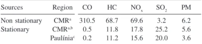
concentrates a very expressive industrial area with potential Hg emission sources, such as the largest Brazilian petroleum refinery, petrochemical and chemical industries, oil derivatives distributors, an Hg recycling industry, incinerators, etc. Table 1 presents some data about atmospheric pollution sources in the CMR.
The region presents a typical sub-tropical climate. In the studied area the monthly mean precipitation and monthly mean air temperature for the dry season (April to September) are 47 mm and 20.5 oC, respectively, with
191 mm and 24.4 oC for the rainy season (October to
March).16 During the dry period, strong anti cyclonic
situations lead to frequent atmospheric stability conditions which are more critical for pollutant dispersion.17
Table 1. Assessment of atmospheric pollutant source emission (1000 t
per year) in the Campinas Metropolitan Region in 2003 (CETESB, 2004)
Sources Region CO HC NOx SO2 PM
Non stationary CMRa 310.5 68.7 69.6 3.2 6.2 Stationary CMRa,b 0.5 11.8 17.8 25.2 5.6 Paulíniac 0.2 11.2 15.6 20.0 3.6
Sampling sites and campaigns
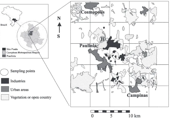
Two sampling points were selected according to the dominant wind direction, which in this region is from southeast to northwest. One point was located on the Campinas State University (Unicamp) campus, which is surrounded by a residential area, about 10 km southeast of the Paulínia industrial area (Figure 1). About 1 km to the south a highway with heavy traffic of cars and trucks is located. The second point was ~3 km east-northeast of the Paulínia industrial district, in a place that directly receives the atmospheric emissions from the industrial district.18
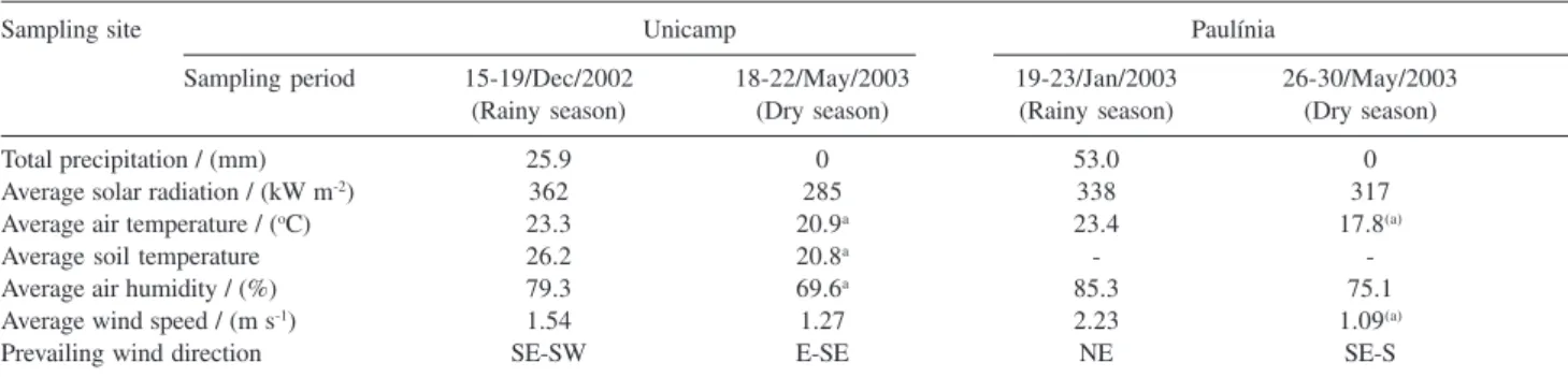
In order to study daily and seasonal variations, two five-days campaigns were performed at each site. The time schedule of each campaign is shown in Table 2. TGM and TPM were simultaneously measured at each site. Some meteorological parameters, such as solar radiation, wind speed, wind direction, air temperature and relative air humidity were obtained from the Unicamp meteorological station, located few hundred meters from the campus sampling point, and from CETESB (Companhia de Tecnologia de Saneamento Ambiental do Estado de São Paulo) station located in Paulínia ~ 2 km south of the sampling point and which also records atmospheric pollutant concentrations.
Sampling and analysis of Total Gaseous Mercury (TGM)
TGM sampling and analysis is based on gold trap amalgamation and subsequent analysis using Cold Vapor Atomic Fluorescence Spectrometry (CVAFS).19 Samples
were collected on 10 cm long traps consisting of a 7 mm (i.d.) quartz tube containing gold-coated quartz glass grains, held in place by quartz wool plugs. Everyday six gold traps were connected by a silicone tube (6 mm i.d.) to a sequential sampler (RAC – Research Appliance Company, mod. PV, serial 509), constituted of a diaphragm pump with air regulator orifice linked to a twelve channel selecting valve connected to a timer. According to the initial program, the timer switches the pumping on and directs the flow to a selected valve position. The inlet to the gold-trap was also connected by a 20 cm Teflon® tube
(7 mm i.d) to a 40 g soda-lime trap in order to protect the gold-trap from air humidity. Air was drawn through the quartz tube at a flow rate around 0.3 L min-1, measured
before and after sampling by a calibrated flowmeter for each sampling channel. The sampling time was 2 h, with 2 h separating two samplings, allowing collection of six samples in each 24 h period. In order to verify the potential passive amalgamation on the gold trap during the 2 h active sampling time, for every 24 h periods, two gold traps (field
blanks) were also connected to the sampling device but without pumping air. TGM traps were placed 1 m above the soil. TGM quantification was performed using an AFS (Brooks Rand – Mod III) after a second amalgamation stage on the analytical column; gold filtered argon was used as carrier gas. The standard curves were prepared daily for the analytical column using injections of known concentrations of Hg saturated air.20 A detection limit of
18 to 65 pg was typically observed.
Sampling and analysis of Total Particulate Mercury (TPM)
TPM was sampled according to the US.EPA method,21 by using a quartz glass filter (Pallflex®,
Tissuquartz®, 0.3 mm porosity and 47 mm diameter),
housed in an open Teflon® filter holder. The flow rate
was around 30 L min-1, and the total sampled volume
was measured by connecting a calibrated gas meter just after the pump outlet. Each sample was collected for 24 h. The filter holder was placed 1 m above the soil. Before use, sampling filters and filter holders were cleaned according to U.S. EPA recommendations.21
After sampling, filters were individually stored in Petri boxes sealed by Teflon ties. Filters were digested in 20 mL of 10% HNO3 with 0.5 mL of BrCl, in order to convert all forms of Hg into the inorganic form, Hg2+.
The remaining BrCl was reduced by NH2OH·HCl. To a 1.0 mL sample aliquot was added 0.5 mL of SnCl2 solution (containing 20% m/v of SnCl2 and 10% v/v concentrated HCl, bubbled with gold filtered argon for 15 min) in order to reduce Hg2+ to Hg0. This solution
was then purged by gold filtered argon to carry the Hg0
to the gold trap. Amalgamated Hg0 was then quantified
by AFS in the same manner as described for TGM. The standard curve was prepared by adding different volumes of a 2 ng mL-1 Hg(II) standard solution to
quartz glass filters, which were then digested and analyzed in the same way as the samples. A detection
limit of 48 pg was observed. Precision and accuracy were checked by the analysis of Certified Reference Material (San Joaquim Soil - NIST)/(CRM = 1.40 ± 0.08 µg g-1 Hg – value obtained 1.36 ± 0.05 µg g-1 Hg).
Statistical analyses
To avoid assuming a given statistical distribution of the values, the nonparametric Mann-Whitney U test was used to test for differences between two data sets and the relation between two variables was analyzed by Spearman rank correlation; the statistical significance was tested at a p-level of 0.05. The statistical software STATISTICA (99 edition) was used to perform these statistical analyses.
Results and Discussion
Total gaseous mercury concentrations
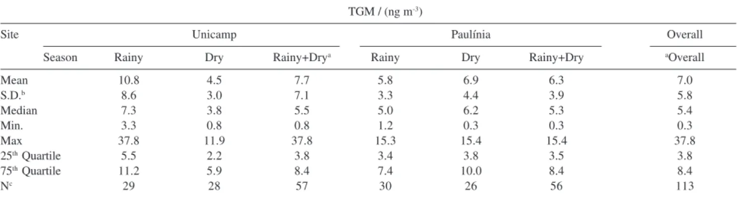
The TGM data obtained for both sampling sites and both seasons are shown in Table 3. The mean TGM concentration ± 1 S.D. calculated for the total period of measurements at both sites was 7.0 ± 5.8 ng m-3. When
considering each sampling site, the mean concentrations were 7.7 ± 7.1 ng m-3 and 6.3 ± 3.9 ng m-3, at Unicamp
and Paulínia, respectively, and no significant difference was found between the two sites. Although one concentration of 90.8 ng m-3 was found at Paulínia during
the dry period, this value was considered an outlier. Thus, the highest concentrations were 37.8 and 15.4 ng m-3,at
Unicamp and Paulínia, respectively.
In a global scale, the concentrations of TGM found in non-contaminated areas vary over a range of 1 to 5 ng m-3.22,23 In Brazil, for measurements performed in the
Negro River Basin (Amazonian region), Fadini and Jardim24
found a median TGM concentration of 1.3 ng m-3 and Magarelli and Fostier25 reported values between
0.4 and 1.4 ng m-3. Artaxo et al.26 reported concentrations
Table 2. Time schedule of each campaign and main atmospheric conditions at Unicamp and Paulínia, during the sampling periods
Sampling site Unicamp Paulínia
Sampling period 15-19/Dec/2002 18-22/May/2003 19-23/Jan/2003 26-30/May/2003 (Rainy season) (Dry season) (Rainy season) (Dry season)
Total precipitation / (mm) 25.9 0 53.0 0
Average solar radiation / (kW m-2) 362 285 338 317
Average air temperature / (oC) 23.3 20.9a 23.4 17.8(a)
Average soil temperature 26.2 20.8a -
-Average air humidity / (%) 79.3 69.6a 85.3 75.1
Average wind speed / (m s-1) 1.54 1.27 2.23 1.09(a)
Prevailing wind direction SE-SW E-SE NE SE-S
from 0.5 to 2 ng m-3 for the Amazonian region. Nevertheless,
as far as we known there is no available data for Brazilian industrialized regions, nor for industrial areas of other South American countries. In contrast, several monitoring campaigns have been carried out in the rest of the world, mainly in the northern hemisphere and the results showed that the proximity of the emitting sources causes a great variability in the TGM concentrations. Poissant,27 for
example, in measurements carried out in agricultural locations around Montreal, generally found low concen-trations, with some points of high concentration (i.e. mean
of 1.79 ng m-3 with a maximum of 57.86 ng m-3). Also with
the proximity of anthropogenic sources, higher TGM concentrations are expected. Dommergue et al.,28 in a
monitoring campaign carried out near (~ 4 km) a chlor-alkali plant found a mean TGM concentration of 3.4 ng m–3,with many peaks above 10.0 ng m–3, and a maximum
of 45.9 ng m–3.Ebinghaus and Krüger,29 in measurements
performed at the perimeter of a chlor-alkali plant, have detected values that ranged from 10 to 530 ng m-3; the
highest concentrations were found at the center of the mercury plume. High values (average ~10 ng m–3)have also
been observed by Kim and Kim30 in Seoul (Korea). Our
data showed that TGM concentrations higher than 10 ng m-3 accounted for 17.5% and 19.6% of the total
measure-ments at Unicamp and Paulínia, respectively. From these results one can conclude that the mean concentrations and the frequency of high values clearly indicate the influence of significant anthropogenic sources of mercury in the Campinas Metropolitan Region.
Diel and seasonal variations of TGM
At Unicamp, TGM concentrations were significantly higher (Mann-Whitney, p < 0.05) during the rainy season while at Paulínia TGM concentrations were not significantly different between the two seasons (Table
3), showing that seasonal variations may be due to the variation of local parameters. Several studies carried out in the northern hemisphere have pointed out seasonal variation in TGM concentrations, some finding a winter maximum and others a summer maximum, but there is no agreement about which season has the highest concentration.31 On the other hand, as far as
we know, TGM seasonal variation has never been studied in a sub-tropical region from the southern hemisphere, with meteorological conditions similar to those found in our study.
Some meteorological parameters were analyzed in order to verify their potential relationship with seasonal TGM concentration variations. In this way, seasonal differences were tested (Mann-Whitney U test, 95%) for wind speed, air temperature, air humidity and solar radiation; prevailing wind direction at each season was also analyzed. As shown in Table 2, the only meteoro-logical parameters that presented a significant difference between the dry and the rainy season at Unicamp were air temperature, air humidity and wind direction, therefore these parameters could be related to the seasonal TGM concentration variations observed at Unicamp. No significant difference was observed for solar radiation. Although solar intensity is typically higher during the summer (rainy season), the lack of significant difference for the solar radiation between the two seasons can probably be explained by the high nebulosity during the rainy season. Air temperature presented a significant difference at Unicamp and at Paulínia, but at Paulínia TGM concentrations were not significantly different between both seasons. For this reason, air temperature could not itself explain the seasonal TGM variation in concentration at Unicamp. Air humidity was also significantly higher during the rainy season. Nevertheless, no correlation was found between air humidity and TGM concentration at Unicamp. Therefore, at Unicamp, wind
Table 3. Summary of TGM data at Unicamp andPaulínia
TGM / (ng m-3)
Site Unicamp Paulínia Overall
Season Rainy Dry Rainy+Drya Rainy Dry Rainy+Dry aOverall
Mean 10.8 4.5 7.7 5.8 6.9 6.3 7.0
S.D.b 8.6 3.0 7.1 3.3 4.4 3.9 5.8
Median 7.3 3.8 5.5 5.0 6.2 5.3 5.4
Min. 3.3 0.8 0.8 1.2 0.3 0.3 0.3
Max 37.8 11.9 37.8 15.3 15.4 15.4 37.8
25th Quartile 5.5 2.2 3.8 3.4 3.8 3.5 3.8
75th Quartile 11.2 5.9 8.4 7.4 10.0 8.4 8.4
Nc 29 28 57 30 26 56 113
direction appears to be the parameter that better explains the TGM seasonal variation. As shown in Figure 2, during the dry season (lower TGM concentrations) wind mainly originated from the east where vegetation and open country dominate (Figure 1). On the other hand, during the rainy season the dominant wind direction was from south where, at about 2 km, a highway with heavy traffic of cars and trucks is located and also where Campinas city is located (Figure 1). No data are available about sources of mercury emissions in the city of Campinas, nor about air quality parameters, however, the higher TGM concentrations observed during the rainy season at Unicamp could be mainly related to the wind trajectory.
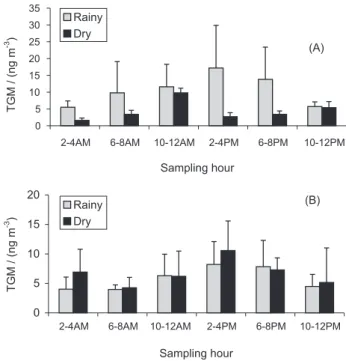
The diel variability of TGM concentration at Unicamp and Paulínia is presented in Figure 3. The highest concentrations of TGM were generally reached during daytime, mainly during the rainy season. Diurnal variations of TGM have already been observed in a number of studies29,32-35 and, in all cases, this pattern is associated with
sites close to TGM emission sources, since the TGM present in air masses from medium and long distances is dissipated. Increases in TGM concentrations during the day could be associated to different factors such as: increase of the anthropogenic emissions, increase of soil degassing, and differences of atmospheric turbulence between day and night. A Spearman matrix correlation was built (Table 4) in order to better understand the possible relationship between
meteorological conditions and TGM concentrations and O3 and TGM concentrations.
As could be expected from the trend of the diurnal variation of TGM concentrations, high correlations (positive or negative) were generally observed with solar radiation and with other parameters that depend on solar radiation, such as air temperature, air humidity and O3. It has already been shown that increases in air temperature and mainly soil temperature can enhance TGM emissions from soils.25,35,36 At Unicamp, the correlation between
TGM concentration and soil temperature (rainy season) was higher than with air temperature, first suggesting that soil emission could be responsible for increasing atmospheric TGM concentration during the day. As far as we know, a direct relationship between soil emission and increase of atmospheric TGM concentration during the day has only been shown by Feng et al.,35 in two suburban
Figure 2. Wind direction frequency at Unicamp and Paulínia during the sampling periods.
Table 4. Sperman correlation coefficients between 2-hour Hg concentra-tions and meteorological parameters and Hg concentration and O3
Unicamp Paulínia
Rainy Dry Rainy Dry
Solar radiation 0.40a 0.20 0.55a 0.26 Air temperature 0.37a -0.13 0.53a 0.44a
Soil temperature 0.58a -0.26 -
-Air humidity 0.06 0.09 -0.68a -0.33
Wind speed 0.02 -0.24 0.46a 0.36
Wind direction 0.23 0.02 0.41 0.24
O3 - - 0.54a 0.43a
aIndicates significant correlation (p<0.05).
areas where soil Hg concentrations were on the order of 220-250 ng g-1,resulting in average TGM concentrations
on the order of 8 ng m-3. Unfortunately, soil Hg
concentrations were not determined in our study. Nevertheless, if one accepts soil degassing as being responsible for diel TGM variations at Unicamp, the lack of correlation during the dry season and also the low atmospheric TGM concentrations could be explained by lower soil temperatures. In their study, Feng et al.35 did
not observe correlations between soil emission and TGM concentrations in two urban areas, although TGM concentrations and soil emissions were of the same order as in the suburban areas. This lack of correlation was attributed to the direct influence of anthropogenic emissions in the urban areas. To sum up, it appears that at Unicamp the diel and seasonal variations could be related to soil emission or to anthropogenic emissions coupled to atmospheric dispersion processes. Nevertheless, the lack of more consistent data, such as Hg concentration in soil and soil Hg emission, do not allow deciding which of these sources could be responsible for the high TGM concentrations observed during the rainy season at Unicamp. On the other hand, diel TGM variations were always observed at Paulínia, which could probably be related to the intense anthropogenic activity (urban and industrial) in this area. The analysis of some atmospheric pollutant concentration data would probably be very helpful in order to verify this hypothesis. Nevertheless, the available data were recorded in Paulínia at a place located ~ 2 km south of the sampling point and perhaps do not integrate the same emission sources as those influencing our sampling point. For this reason, it would not make sense to build a correlation matrix between this data and TGM concentrations. Nevertheless, in order to give an idea about atmospheric quality in Paulínia, the concentrations of O3, NO2, SO2, CO and MP10 were analyzed in view of the Brazilian regulations. It appeared that during the monitored periods these pollutants were always lower than the concentrations defined as giving a low-level health effect.
Total Particulate Mercury concentrations
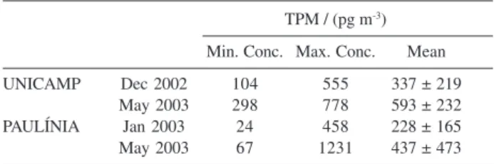
The TPM concentration data obtained during the sampling campaigns are shown in Table 5. The mean TPM concentration calculated for the total period of sampling was 465 (± 252) pg m-3 at Unicamp and 332 (± 351) pg m-3
at Paulínia. These values are of the same order of magnitude as those found by Fang et al.37 in an industrial
district of China (22 pg m-3 to 1984 pg m–3), and also
comparable to the TPM concentrations in urban/
industrialized areas of the United States, which ranged from 15 pg m-3 to 1200 pg m-3.38 According to Keeler et al. 38 background values for TPM concentrations typically
vary from 1 pg m-3 to 86 pg m-3. In the north of the Europe,
the highest TPM concentrations found by Wängberg et al.12 ranged from 5 pg m-3 to 200 pg m-3. According to
theses authors, these areas receive influences from anthropogenic sources of Europe, since particulate mercury can be carried on regional scale to distances from 500 to 800 km.
Although TPM concentrations were not significantly different between seasons, probably due to the high variability of the data, the highest TPM values were detected during the dry period at both sites (778 at Unicamp and 1231 pg m-3 at Paulínia). These could be
related with the pluvial index: 25.9 mm (being 9.9 mm on the first day of sampling) at Unicamp and 53.0 mm at Paulínia during the wet period and 0 mm at both Unicamp and Paulínia during the dry period. Rain drags the existing particulate material in air to the ground (wet deposition), contributing to the removal of these particles from the atmosphere.
In this work, the percentage of TPM in relation to total atmospheric mercury was calculated, assuming that total atmospheric mercury is given by the sum of TGM and TPM. The calculated percentage of TPM was 4.5% (wet) and 12.2% (dry) at Unicamp and 3.3% (wet) and 4.9% (dry) at Paulínia. These results may be compared with those expected for TPM/TGM concentrations in industrialized regions, where TPM can constitute up to 40% of the total atmospheric mercury, while in remote areas TPM contributes less than 1% of the total atmospheric mercury.7,9
Conclusions
In Brazil some measurements of atmospheric mercury concentrations have been performed in the Amazonian region, but as far as we know, our results are the first reported about atmospheric mercury concentrations in a highly industrialized Brazilian region. The data clearly showed that TGM and TPM
Table 5. TPM concentration data for the sampling campaigns
TPM / (pg m-3)
Min. Conc. Max. Conc. Mean
UNICAMP Dec 2002 104 555 337 ± 219
May 2003 298 778 593 ± 232
PAULÍNIA Jan 2003 24 458 228 ± 165
concentrations are on the same order of magnitude as those found in industrialized regions in the northern hemisphere. Although in Brazil, as in many other developing countries, gold mining activities have been considered as the main sources of mercury emission, our results showed that other anthropogenic sources, such as fossil fuel combustion, can also significantly enhance atmospheric mercury concentrations. Nevertheless, probably due to the limited quantity of our data, it was not possible to point to a main mercury emission source, and our study also shows the need for further research about soil emission. Our study points out the need for more monitoring campaigns and also the need for assessment of anthropogenic mercury emission sources in Brazilian industrial regions. Our data also show that emissions from the most industria-lized Brazilian regions, and probably from similar regions in other countries of the southern hemisphere, should be assessed and integrated into the global anthropogenic mercury emission assessment.
Acknowledgments
The authors would like to acknowledge FAPESP for financial support (FAPESP N02000/11508-5), CNPq and
FAEP for a MSc thesis grant (CNPq No 131632-2001-9; FAEP No 665/03), CETESB for sampling orientation and
the loan of sequential sampler and Dr. Carol H. Collins for English revision.
References
1. Bisinoti, M. C.; Jardim, W. F; Quim. Nova2004, 27, 593.
2. WHO (World Health Organization); Air Quality Guidedlines,
2nd ed., 2000.
3. Slemr, F.; Schuster, G.; Seiler, W.; J. Atmos. Chem.1985, 3,
407.
4. Lindqvist, O.; Rodhe, H.; Tellus1985, 37B, 136.
5. Schroeder, W. H.; Munthe, J.; Atmos. Environ.1998, 32, 809.
6. UNEP (United Nations Environmental Programme); Global
Mercury Assessment, Geneva, Suíça, 2002.
7. Munthe, J.; Wängberg, I.; Pirrone, N.; Iyerfeldt, Å.; Ferrara, R.; Ebinghaus, R.; Feng, X.; Gårdfeldt; Keeler, G.; Lanzillotta; Lindberg, S. E.; Lu, J.; Mamane, Y.; Prestbo, E.; Schmolke, S.; Schroeder, W. H.; Sommar, J.; Sprovieri, F.; Stevens, R. K.; Stratton, W.; Tuncel, G.; Urba, A.; Atmos. Environ.2001, 35,
3007.
8. Munthe J.; McElroy W. J.; Atmos. Environ.1992, 26, 553.
9. Lin, C-J.; Pehkonen, S. O.; Atmos. Environ.1999, 33, 2067.
10. Pilgrim, W.; Poissant, L.; Trip, L.; Sci. Total Environ.2000,
261, 177.
11. Pilgrim, W.; Schroeder, W.; Porcella, D.B.; Santos-Burgoa, C.; Montgomery, S.; Hamilton, A.; Trip, L.; Sci. Total Environ.
2000, 261, 185.
12. Wängberg, I.; Munthe, J.; Pirrone, N.; Iverfeldt, Å.; Bahlman, E.; Costa, P.; Ebinghaus, R.; Feng, X.; Ferrara, R.; Gårdfeldt, K.; Kock, H.; Lancillota, E.; Mamane, Y.; Mas, F.; Melamed, E.; Osnat, Y.; Prestbo, E.; Sommar, J.; Schmolke, S.; Spain, G.; Sprovieri, F.; Tuncel, G.; Atmos. Environ.2001, 35, 3019.
13. Ramel, C. In Global and Regional Mercury Cycles, NATO
Advanced Science Institute Serie; Ebinghaus, R.; Bayens, W.;
Vasiliev, O., eds.; Kluwer: Dordrecht, 1996, p. 505.
14. Brazil, 2003: Brazilian Energy Balance, Secretariat for Energy,
Ministry of Mines and Energy: Brasilia, 2003, p. 168. 15. Emplasa (Empresa Paulista de Planejamento Metropolitana);
Sumário de Dados da Região Metropolitana de Campinas
(CD-ROM), Emplasa: Campinas, 2002.
16. Cepagri, 2004. http://www.cpa.unicamp.br, accessed in September 2004.
17. CETESB (Companhia de Tecnologia de Saneamento Ambiental); Relatório de Qualidade do Ar do Estado de São
Paulo 2003, São Paulo, 2004, p. 137.
18. Tomaz, E.; Clemente, D. A.; Proceedings of the Sixth International Conference on Technologies and Combustion for
a Clean Environment - CLEANAIR 2001, Oporto. CLEANAIR,
2001, vol. 3, p. 1529.
19. Bloom, N. S., Fitzgerald, W. F.; Anal. Chim. Acta1998, 209,
151.
20. Dumarey, R.; Temmerman, E.; Dams, R.; Hoste, J.; Anal. Chim. Acta1985, 170, 337.
21. U.S.EPA; Sampling and Analysis for Atmospheric Mercury,
EPA/625/R-96/010a, 1999.
22. Lee, D. S.; Dollard, G. J.; Pepler, S.; Atmos. Environ.1998, 32,
855.
23. Ebinghaus, R.; Jennings, S. G.; Schroeder, W.; Berg, T.; Donahy, T.; Guentzel, J.; Kenny, C.; Kock, H. H.; Kvietkus, K.; Landing, W.; Mühleck, T.; Munthe, J.; Prestbo, E. M.; Schneeberger, D.; Slemr, F.; Sommar, J.; Urba, A.; Wallschläger, D.; Xiao, Z.;
Atmos. Environ.1999, 33, 3063.
24. Fadini, P.; Jardim, W. F.; Sci. Total Environ.2001, 275, 71.
25. Magarelli, G., Fostier A. H.; Atmos. Environ.2005, 39, 7518.
26. Artaxo, P.; de Campos, R. C.; Fernandes, E. D.; Martins, J. V.; Xiao, Z.; Lindqvist Å; Fernandez-Jimenez, M. T.; Maenhaut,
W; Atmos. Environ.2000, 34, 4085.
27. Poissant, L.; Sci. Total Environ. 2000, 259, 191.
28. Dommergue, A.; Ferrari, C. P.; Planchon, F. A. M.; Bouton, C. F.; 2002. Sci. Total Environ.2002, 297, 203.
29. Ebinghaus, R.; Krüger, O. In Global and Regional Mercury
Cycles, NATO Advanced Science Institute Serie; Ebinghaus,
R.; Bayens, W.; Vasiliev, O., eds.; Kluwer: Dordrecht, 1996, p. 135.
31. Han, Y-J.; Holsen, T. M.; Lai, S-O.; Hopke, P. K.; Yi, S-M.; Liu, W.; Pagano, J.; Falanga, L.; Milligan, M.; Andolina, C.;
Atmos. Environ.2004, 38, 6431.
32. Kvietkus, K.; Sakalys, J. In Mercury Pollution: Integration and
Synthesis; Watras, C.J.; Huckabee, J.W., eds., CRC Press : Boca
Raton, 1994.
33. Schmolke S. R.; Schroeder W. H.; Kock H. H.; Schneeberger D.; Munthe J.; Ebinghaus R.; Atmos. Environ.1999, 33, 1725.
34. Kim, K. H.; Kim, M. Y.; Atmos. Environ. 2002,36, 4914.
35. Feng, X.; Wang, S.; Qiu, G.; Hou, Y.; Tang, S.; J. Geophys. Res.2005, 110, D14, D14306.
36. Lindberg, S. E.; Kim, K. H.; Meyers, T. P.; Owens, J. G.;
Environ. Sci. Technol.1995, 29, 126.
37. Fang, F.; Wang, Q.; Liu, R.; Ma, Z.; Hao, Q.; Atmos. Environ.
2001, 35, 4265.
38. Keeler, G. J.; Glinsorn, G.; Pirrone, N.; Water Air Soil Pollut.
1995, 80, 159.
Received: January 24, 2006 Published on the web: June 20, 2006