Appendix A
Option Valuation Formulas
A.1
Discrete Average Price Asian Call
It is possible to value asian options using regular BS model’s option pricing formulas if we assume the average priceSavg to have a log-normal distribution just like a regular
price series. A geometric price average however does follow a log-normal distribution, while an arithmetic average follows a log-normal distribution approximately.
If that is the case and we take the average price series to be log-normal, there is an adjustment [10] that can be made to the Black-Scholes futures option pricing formula in (A.3), which yields the price of a continuously average price asian option. However in this case, since we are only considering close price series in testing simulations, we are interested to choose the time instants at which the average is calculated. There is a formula to do it, however an extra step is required since we are valuing the options with passed averaging observations that will contribute as well to the final option payoff. This is possible by adjusting the strike according to the price average ¯Sverified in the periodt1
that have passed [11], as in:
K∗=t1+t2 t2
K−t1 t2
¯
S (A.1)
where K is the actual strike of the asian option and t2 is the period of time left until
maturity. According to the value of K∗ different pricing formulas (A.2) and (A.3) are used:
CK∗≤0= t2 t1+t2
(M1−K∗)e−rt2 (A.2) CK∗>0= [F0N(d1)−K∗N(d2)]e−rt2 (A.3)
These formulas require the variable adjustments described below:
F0=M1 , M1=
1
m m
∑
i=1
Fi , Fi=Ste(r− δt)Ti
A.1. DISCRETE AVERAGE PRICE ASIAN CALL
the current priceSt to nextith observation. d1=
ln
F0
K∗
+σ22t2
σ√t2 , d2=d1−σt2 , σ
2= 1 Tln
M2 M12
M2= 1 m2
m
∑
i=1
Fi2eσi2Ti+2 m
∑
j=1 j−1
∑
i=1
FiFjeσi2Ti
!
A.1.1
Vanilla Call
C=Se−δTN(d1)−Ke−rTN(d2) (A.4)
d1=
ln KS+r−δ+σ2
2
T
σ√T , d2=d1−σ
√ T
A.1.2
Binary Call
The binary call formula is just the discountedCoupontimes the probabilityN(d2)of being paid.
C=Coupon×e−rTN(d2) (A.5)
A.1.3
Up-and-In Call
As one could tell by looking at Fig.(3.1) the european Up-and-In option used in this work has can be thought as composed by a OTM binary option plus a OTM vanilla call option with strikeH >K. Since the BS model assumes constant volatility, the volatility used can be the same as the one used for the ATM vanilla and binary call. Normally when pricing OTM or ITM options one would have to increase volatility due to the volatility smile.
C=Se−δTN(d1)−He−rTN(d2) + (H−K)e−rTN(d2) =Se−δTN(d1)−Ke−rTN(d2)
(A.6)
d1=
ln HS+r−δ+σ2
2
T
σ√T , d2=d1−σ
Appendix B
Experimental Results Figures
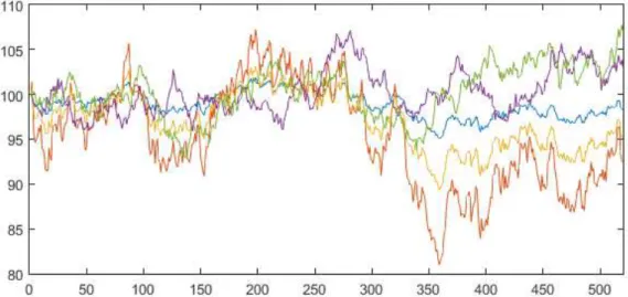
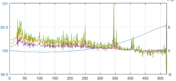
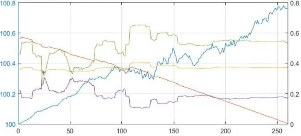
The following graphs support chapter 4. All graphs units in thex-axis are expressed in days, and iny-axis expressed in absolute values, unless stated otherwise. As for the price series a generic price of 100 was chosen forS0, as one can tell by looking at the graphs.
Some graphs will contain twoy series, which although having different scales share the same unit. Apart from the caption, below each graph one also can find the reference to the table containing the information for that particular test, if there is one, as well as the parameters used for the test, which if absent were set to zero.
Figure B.2: Average daily price and Delta Hedging PnL w/σ =10% andr=−0.5%
Price(Left Axis);Asian;Vanilla;Binary;UpAndIn(Right Axis); Table (C.2)
Figure B.3: Average daily price and Delta Hedging PnL w/σ =25% andr=1.0%
Price(Left Axis);Asian;Vanilla;Binary;UpAndIn(Right Axis); Table (C.3)
Figure B.4: Average daily deltas w/σ=25% andr=1.0%
Figure B.5: Average option and underlying price w/σ =20%,r=1.0% andδ =4.0%
Price(Left Axis);Asian;Vanilla;Binary;UpAndIn(Right Axis); Table (C.4)
Figure B.6: Real Annual Interest Rate that would be used in a 2 year Option started at 02/01/2014.yvalues in percentage points.
Figure B.7: Average price and Hedging PnL w/σ =10%,r=real
Figure B.8: Average price and Hedging PnL w/σ =10%,rinverse trend of real
Price(Left Axis);Asian;Vanilla;Binary;UpAndIn(Right Axis); Table (C.6)
Figure B.9: Average price and Hedging PnL w/σ =10%,rinverse trend of real
Price(Left Axis);Asian;Vanilla;Binary;UpAndIn(Right Axis); Table (C.7)
Figure B.10: Volatility series and Hedging PnL w/σ=real,r=1%
Figure B.11: Average Price and Delta series w/σ =real,r=1%
Price(Left Axis);Asian;Vanilla;Binary;UpAndInDeltas (Right Axis); Table (C.8)
Figure B.12: Close up of Fig.(B.10)
Volatility(Left Axis);Asian;Vanilla;Binary;UpAndIn(Right Axis);
Figure B.13: t-distributionwith 5 degrees of freedom;
Appendix C
Experimental Results Tables
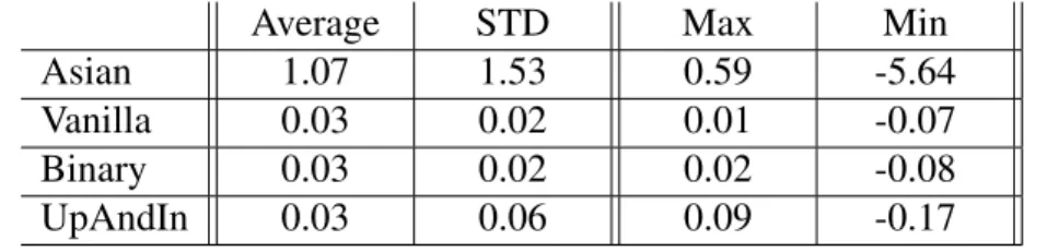
The following tables support chapter 4. The tables mostly contain figures regarding averages, annualised standard deviations, maximum and minimum values expressed in basis points, unless stated otherwise. Values for Kurtosis and Skewness are unitless.
Average STD Max Min Asian 1.07 1.53 0.59 -5.64 Vanilla 0.03 0.02 0.01 -0.07 Binary 0.03 0.02 0.02 -0.08 UpAndIn 0.03 0.06 0.09 -0.17
Table C.1: Option princing difference between Closed Formula and Monte Carlo.
σ =10%,r=−0.5% andT =520
Average STD Kurtosis Skewness Max Min Asian 0.18 10.79 60.09 4.45 9.25 -0.56 Vanilla 0.22 11.70 22.62 3.34 9.93 -0.55 Binary 0.14 12.12 25.11 1.79 11.97 -10.05 UpAndIn 0.28 31.98 38.66 4.26 36.88 -12.40
Table C.2: Delta Hedging PnL.
σ =10%,r=−0.5% andT =520
Average STD Kurtosis Skewness Max Min Asian 0.48 44.91 31.53 3.82 36.68 -2.58 Vanilla 0.59 48.65 21.02 3.31 39.01 -2.45 Binary 0.38 44.74 25.89 2.23 42.05 -33.72 UpAndIn 0.76 131.29 37.80 4.24 141.99 -40.22
Table C.3: Delta Hedging PnL.
Dividends 4 2 Asian 40.38 37.96 Vanilla 50.63 37.55 Binary 29.30 22.09 UpAndIn 66.62 49.08
Table C.4: Average Delta Hedging PnL without and with dividend cuts.
σ=20%,r=1.0%,T =260,δ =4.0%
Average STD Kurtosis Skewness Max Min Asian 0.00 10.63 69.26 4.76 8.93 -0.77 Vanilla 0.02 11.28 22.59 3.30 9.28 -0.77 Binary 0.02 12.42 26.81 1.45 12.13 -11.12 UpAndIn 0.02 34.32 37.76 4.04 39.00 -14.84
Table C.5: Delta Hedging PnL.
σ=10%,T =520, andr=real
Average STD Kurtosis Skewness Max Min Asian 0.11 10.63 66.08 4.80 9.11 -0.65 Vanilla 0.11 11.49 23.15 3.36 9.63 -0.66 Binary 0.07 12.11 26.08 1.55 11.81 -10.72 UpAndIn 0.14 33.04 36.46 4.03 36.98 -13.44
Table C.6: Delta Hedging PnL.
σ =10%,T =520, andrequal to the inverse trend of real
Average STD Kurtosis Skewness Max Min Asian -0.95 18.71 11.60 -1.33 7.86 -8.13 Vanilla -0.94 19.74 6.60 -0.38 8.46 -8.19 Binary -0.79 23.13 7.23 -1.09 10.21 -14.39 UpAndIn -2.12 62.71 8.56 -1.00 32.18 -35.08
Table C.7: Delta Hedging PnL with 1 basis point bid-ask spread.
σ =10%,T =520, andrequal to the inverse trend of real
Average STD Kurtosis Skewness Max Min Asian 5.27 271.28 32.24 3.57 223.63 -17.26 Vanilla 6.59 325.70 26.80 3.07 289.33 -22.12 Binary 1.95 365.60 12.23 1.15 124.66 -87.21 UpAndIn 10.34 892.03 30.64 2.81 645.78 -151.61
Table C.8: Delta Hedging PnL with real volatility series.
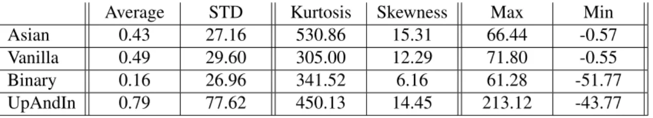
Average STD Kurtosis Skewness Max Min Asian 0.43 27.16 530.86 15.31 66.44 -0.57 Vanilla 0.49 29.60 305.00 12.29 71.80 -0.55 Binary 0.16 26.96 341.52 6.16 61.28 -51.77 UpAndIn 0.79 77.62 450.13 14.45 213.12 -43.77
Table C.9: Delta Hedging PnL with t-distributed returns.
σ =10%,r=−0.5% andT =520
Average STD Kurtosis Skewness Max Min Asian -37.13 681.85 32.27 3.79 36.71 -283.39 Vanilla -58.09 926.47 20.22 3.22 39.18 -446.19 Binary -31.07 323.94 25.99 2.11 41.71 -85.97 UpAndIn -81.59 1974.38 34.88 4.08 148.37 -804.57
Table C.10: Delta Hedging PnL with a negative price shock.