Georgeto SM et al. / Comparison between T1 GRE and T1 IR GRE MRI sequences
Radiol Bras. 2016 Nov/Dez;49(6):382–388 382
Original Article
T1-weighted gradient-echo imaging, with and without
inversion recovery, in the identification of anatomical
structures on the lateral surface of the brain
*
T1 GRE e T1 IR GRE na identificação das estruturas anatômicas da face lateral do cérebro
Georgeto SM, Zicarelli CAM, Gariba MA, Aguiar LR. T1-weighted gradient-echo imaging, with and without inversion recovery, in the identification of anatomical structures on the lateral surface of the brain. Radiol Bras. 2016 Nov/Dez;49(6):382–388.
Abstract
R e s u m o
Objective: To compare brain structures using volumetric magnetic resonance imaging with isotropic resolution, in T1-weighted gradient-echo (GRE) acquisition, with and without inversion recovery (IR).
Materials and Methods: From 30 individuals, we evaluated 120 blocks of images of the left and right cerebral hemispheres being acquired by T1 GRE and by T1 IR GRE. On the basis of the Naidich et al. method for localization of anatomical landmarks, 27 anatomical structures were divided into two categories: identifiable and inconclusive. Those two categories were used in the analyses of repeatability (intraobserver agreement) and reproducibility (interobserver agreement). McNemar’s test was used in order to compare the T1 GRE and T1 IR GRE techniques.
Results: There was good agreement in the intraobserver and interobserver analyses (mean kappa > 0.60). McNemar’s test showed that the frequency of identifiable anatomical landmarks was slightly higher when the T1 IR GRE technique was employed than when the T1 GRE technique was employed. The difference between the two techniques was statistically significant.
Conclusion: In the identification of anatomical landmarks, the T1 IR GRE technique appears to perform slightly better than does the T1 GRE technique.
Keywords: Magnetic resonance imaging; Brain/anatomy & histology; Reproducibility of results.
Objetivo: Comparar os resultados de identificação de estruturas cerebrais utilizando imagens volumétricas isotrópicas por ressonância magnética, nas aquisições T1 GRE e T1 IR GRE.
Materiais e Métodos: Foram avaliados 120 blocos de imagens, de 30 indivíduos, com imagens extraídas dos hemisférios cerebrais esquerdo e direito, pelos dois métodos de aquisição: T1 GRE e T1 IR GRE. Com base no método de Naidich et al. para localização dos referenciais anatômicos, 27 estruturas anatômicas foram classificadas em duas categorias – identificável versus deixam dúvidas quanto à identificação somadas às não identificáveis – para análises de repetitividade (intraobservador) e reprodutibilidade (interobservadores). Foi utilizado o teste de McNemar para a avaliação do desempenho entre os dois métodos.
Resultados: Após confirmação de ter havido boa concordância na análise intraobservador e interobservadores (kappa médio > 0,60), a avaliação das imagens de cada referencial anatômico, testada entre T1 GRE e T1 IR GRE pelo teste de McNemar, indicou maior frequência de referenciais identificáveis pelo método T1 IR GRE do que pelo método T1 GRE.
Conclusão: O método de imagem T1 IR GRE apresentou desempenho levemente superior, porém estatisticamente significante, em relação ao método T1 GRE, na identificação dos referenciais anatômicos cerebrais.
Unitermos: Ressonância magnética; Estruturas anatômicas cerebrais; Anatomia por imagens de ressonância magnética.
* Study conducted at the Pontifícia Universidade Católica do Paraná (PUCPR), Curitiba, PR, Brazil.
1. Neurosurgeon at the Irmandade da Santa Casa de Londrina and in the De-partment of Neurosurgery at the Universidade Estadual de Londrina (UEL), Londrina, PR, Brazil.
2. Professor in the Graduate Program in Health Technology at the Pontifícia Universidade Católica do Paraná (PUCPR), Curitiba, PR, Brazil.
Mailing address: Dr. Sergio Murilo Georgeto. Avenida Bandeirantes, 476, Vila Ipiranga. Curitiba, PR, Brasil, 86010-020. E-mail: [email protected].
Received March 4, 2015. Accepted after revision December 17, 2015.
netic resonance imaging (MRI). The new CT scanners, with multiple detectors, have good spatial resolution and make it possible to draw correlations with craniometric points. The disadvantages of those CT scanners are the higher dose of radiation emitted and the lower resolution of images of the cortical mantle(1). Studies comparing CT and MRI in terms of their ability to discern the anatomical structures of the lateral surface of the brain have shown that T1-weighted, spin-echo MRI sequences are superior to CT scans for the iden-tification of predetermined structures(2).
Because there are no suitable bone landmarks to facili-tate the MRI localization of the elements of the lateral sur-face of the brain, a system of identifying sulci and gyri was
Sergio Murilo Georgeto1, Carlos Alexandre Martins Zicarelli1, Munir Antônio Gariba2, Luiz Roberto Aguiar2
INTRODUCTION
mag-developed in order to study normal anatomical relationships. The use of a sagittal section of the lateral fissure at its deep-est extent, together with the application of the method for identification of sulci and gyri on the lateral surface, has been found to be particularly successful in the characterization of preselected anatomical elements in T1- and T2-weighted spin-echo MRI sequences(3).
Recent advances in techniques of acquisition and post-processing of images have allowed the acquisition of T1-weighted gradient-echo and T1-T1-weighted gradient-echo with inversion recovery (T1 GRE and T1 IR GRE, respectively) pulse sequences to be employed in routine exams, the cap-ture times no longer representing a financial hindrance to their use. With the improvement in coils and image post-processing methods, it became possible to obtain images from three-dimensional matrices of isotropic voxels, which im-proved the quality of reconstructions in any orthogonal plane. These images are referred to as volumetric sequences with isotropic resolution(4).
The images obtained by T1 GRE have routinely been used in order to demonstrate changes in the cortical topog-raphy in most MRI studies. However, the T1 IR GRE im-ages provide better contrast between gray and white matter, allowing greater accuracy in the identification of anatomi-cal landmarks(5).
The present study aimed to evaluate the identification of anatomical landmarks, using MRI scans of the lateral sur-face of the brain, with pulse sequences that can currently be used for topographic localization. The T1 GRE and T1 IR GRE weightings were selected because the former is routinely used in most MRI scans and the latter is not usually indi-cated for the evaluation of structures of the cortical mantle. If the T1 IR GRE technique could be shown to be superior to that of T1 GRE, it would be a useful finding, because anatomical topography studies of the sulci and gyri that com-prise the cerebral cortex are of interest not only for profes-sionals involved in the diagnosis and treatment of diseases affecting these areas, in terms of the practical aspect of their daily routine(6), but also for neuroscientists who draw ana-tomical and functional correlations between cortical patterns and the development of diseases(7).
The objective of this study was to analyze the perfor-mance of pulse sequences obtained with the T1 GRE and T1 IR GRE techniques. To that end, it was necessary to as-sess, initially, the reliability of the techniques for the method chosen, through analysis of intraobserver and interobserver agreement, and subsequently to compare the performance of the two techniques in order to show which might be more capable of identifying the anatomical landmarks of the lat-eral surface of the brain.
MATERIALS AND METHODS
The study was approved by the Research Ethics Com-mittee of the Pontifícia Universidade Católica do Paraná. All participating subjects gave written informed consent. In
an initial interview, potentially eligible participants com-pleted a questionnaire that included a hand dominance in-ventory (the Edinburgh handedness inin-ventory).
Subjects who showed any neurological changes were ex-cluded, as were those with any other clinical conditions that would preclude the examination. After the initial interview, eligible individuals were referred for MRI at a scheduled day and time. The sample consisted of 30 young adults, with a mean age of 25.3 years; 16 (53.3%) were female, and 14 (46.7%) were male.
The MRI scans were obtained in a 1.5 T scanner (Mag-netom Symphony; Siemens, Erlangen, Germany), with 12-channel coil. The volumetric sequences with isotropic reso-lution were obtained with T1 GRE and T1 IR GRE sequences. For the T1 GRE sequence, we used sagittal gradient-echo volumetric acquisition, with a 256 × 256 matrix, isotropic voxel (1 × 1 × 1 mm), repetition time/echo time (TR/TE) of 1910/3.09 ms, field of view (FOV) of 256 mm, slice thick-ness of 1 mm, no intervals between slices, and a flip angle of 15°. For the T1 IR GRE sequence, we used coronal volu-metric acquisition, with a 256 × 256 matrix, isotropic voxel (1 × 1 × 1 mm), TR/TE of 4000/373 ms, FOV of 260 mm, slice thickness of 1 mm, no intervals between slices, and an inversion time of 350 ms. The Magnetom Symphony scan-ner is equipped with a Quantum gradient (30 mT/m), with a slew rate of 150 mT/ms. A flip angle of 15° was chosen on the basis of data in the literature(8). The remaining param-eters have been used routinely at the radiology clinic where the images were obtained and were in accordance with the manufacturer’s recommendations.
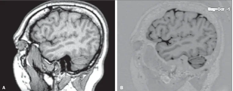
An experienced radiologist analyzed the scans, with the goal of excluding images with motion artifacts or that were inappropriate for evaluation, as well as identifying pathologi-cal findings. The files for all 30 T1 and T1 IR GRE-weighted MRIs of the brain were transferred to OsiriX M.D. software, version 5.7.1, 64-bit (Pixmeo SARL, Bernex, Swit-zerland). Thus, 60 image blocks were formed, and the right and left hemispheres were analyzed separately, resulting in a total of 120 blocks. The images obtained in each of the sequences can be seen in Figure 1.
The anatomy of the lateral surface of the brain was as-sessed qualitatively as to the identification of the major ana-tomical structures, and the method described by Naidich et al.(3), which consists in the description of 15 steps (or signs) for the identification of 27 anatomical structures that com-pose the lateral surface of the brain on MRI slices obtained in the sagittal plane, was used as a reference.
the brain, as described in the most recent study conducted by Naidich et al.(3). For the identification of structures, three categories were considered (Table 1): easily identifiable; inconclusive; and unidentifiable.
Observer 1 analyzed the repeatability of the 120 image blocks in triplicate, with a minimum interval between ob-servations of 10 days, and the observation sequences of the groups of 120 images were randomly recoded at each time Figure 1. Sagittal images of the lateral fissure at its deepest extent, obtained with the T1 GRE (A) and T1 IR GRE (B) techniques.
A B
Table 1—Anatomical landmarks to be identified on the lateral surface of the brain.
Anatomical structures
1. The lateral convexity (sagittal view) in the segment where the deepest extent of the lateral fissure can be seen
2. Lateral fissure
2.1. Posterior horizontal ramus 2.2. Anterior horizontal ramus 2.3. Anterior ascending ramus 2.4. Posterior ascending ramus 2.5. Posterior descending ramus 2.6. Anterior subcentral sulcus 2.7. Posterior subcentral sulcus 2.8. Transverse temporal sulcus 2.9. Anterior sylvian point 3. Inferior frontal gyrus
3.1. Orbital part 3.2. Triangular part 3.3. Opercular part 4. Inferior frontal gyrus
5. Connection between the middle frontal and precentral gyrus 6. Precentral sulcus
7. Precentral gyrus 8. Central sulcus 9. Postcentral gyrus 10. Postcentral sulcus
11. Posterior ascending ramus of the lateral fissure/supramarginal gyrus 12. Superior temporal sulcus
13. Angular gyrus 14. Intraparietal sulcus 15. Superior parietal lobe
Easily
identifiable Inconclusive Unidentifiable
Step 1
Step 2
Step 3
Step 4 Step 5 Step 6 Step 7 Step 8 Step 9 Step 10 Step 11 Step 12 Step 13 Step 14 Step 15
point. That resulted in 360 observations (30 individuals × 2 cerebral hemispheres × 2 imaging techniques × 3 evalua-tions) for the intraobserver analysis.
Two other evaluators (observers 2 and 3) analyzed the anatomical structures. The observers were practicing neurosurgeons and were invited to participate because of their familiarity with the anatomy and corresponding images of the region in question. Those procedures resulted in 240 additional observations (30 individuals × 2 cerebral hemi-spheres × 2 imaging techniques × 2 observers). However, in the reproducibility analysis, we also used the first assess-ment of the researcher, resulting in another 120 comassess-ments. Therefore, a total of 360 observations were used in the interobserver analysis.
All of the observers received an instruction manual with relevant information about the variables to be assessed, an explanation of its use, and tables in which to note their find-ings. The image sequences were all displayed in an standard-ized manner on an Apple MacBook Pro notebook with a 15" screen with retina display, 2880 horizontal pixels, 1800 ver-tical pixels, and 220 ppi resolution. The sequence of 120 image blocks was randomly reordered in three different modes, and each observer had access only to their own data sequence.
The performance of the T1 GRE and T1 IR GRE imag-ing techniques was assessed in two stages: we initially ascer-tained whether the two techniques led the observers to simi-lar results, as determined by analysis of agreement based on the kappa index, and subsequently established the agreement of results between the observers. We then attempted to de-termine whether either technique was able to identify the anatomical structures more easily than was the other. To that end, we used McNemar’s nonparametric test. For the im-age processing in the second stim-age, six different scenarios were taken into account.
RESULTS
In the analysis of intraobserver and interobserver agree-ment, weighted kappa statistics were estimated for each of the three categories: easily identifiable; inconclusive; and uni-dentifiable. Of the 216 potential kappa statistics—for 27 ana-tomical structures, in duplicate (right and left sides); for T1 GRE and T1 IR GRE sequences; and for the intraobserver and interobserver analyses—it was possible to estimate 115: 58 from the intraobserver analysis and 57 from the interob-server analysis.
In general, all kappa statistics were significant at the 1% level, indicating that the agreement among virtually all evaluations was positive and different from zero. Only one kappa statistic—for the interobserver analysis of the perfor-mance of the T1 GRE technique in identifying the anterior subcentral sulcus on the right side—was less than statisti-cally significant (0.04). The mean of the kappa statistics calculated was 0.62 ± 0.02, which is considered indicative of good agreement(9).
According to the criteria established by Byrt et al.(9), only 24.3% of our kappa statistics were classified as poor (< 0.2) or weak (< 0.4). There were no statistical differences be-tween the intraobserver and interobserver analyses: the mean kappa was 0.60 ± 0.03 for the intraobserver analysis and 0.63 ± 0.04 for the interobserver analysis.
After good intraobserver and interobserver agreement had been confirmed, McNemar’s test was carried out in or-der to determine whether either technique was superior to the other in its ability to identify the anatomical structures under study. In conducting McNemar’s test, we assumed that each evaluation of an image of an anatomical structure was independent of the other. Our hypothesis that the evaluations were independent can be considered strong because of the characteristics of the study data, such as individual evalua-tors, individual images, and different time points, which could indicate dependency among the cases. However, if the re-sults remain stable in the various simulations, one could conclude, on the basis of the evidence, in favor of the find-ings obtained.
Theoretically, there would have been 16,200 observa-tions: 8,100 for the T1 GRE technique and 8,100 for the T1 IR GRE technique. That is because the observations col-lected—3 (from observer 1) + 1 (from observer 2) + 1 (from observer 3) = 5 × 120 image blocks = 600—were multiplied by the number of anatomical structures analyzed (27 × 600 = 16,200) and divided by the number of techniques evalu-ated (16,200 / 2 = 8,100). However, two anatomical land-marks—the lateral convexity and the sylvian fissure—were excluded from the results because they presented 100% agree-ment in the intraobserver and interobserver analyses. That was done so as not to overestimate the frequencies of identi-fiable images, given that those two structures are easily iden-tifiable with any technique. Consequently, only 15,000 ob-servations (7,500 each for the T1 GRE and T1 IR GRE tech-niques) were evaluated.
Those observations were submitted to McNemar’s test in six scenarios: 1) all observations (n = 15,000); 2) only
the observations considered in the intraobserver analysis (n
= 9,000); 3) only the observations considered in the interob-server analysis (n = 9,000); 4) only the first observations made
by observer 1 (n = 3,000); 5) only the observations made by
observer 2 (n = 3,000); and 6) only the observations made
by observer 3 (n = 3,000).
T1 IR GRE techniques, in six different scenarios. It should be borne in mind that the unidentified group is the sum of the frequencies of structures categorized as (identification) inconclusive and of those categorized as unidentifiable. Those frequencies are summarized in Table 2.
Of the identifiable images in all observations, 91% were identifiable with the T1 IR GRE technique and 88.8% were identifiable with the T1 GRE technique (McNemar’s χ2
= 77.51; p = 0.000), indicating that the T1 IR GRE technique
features significantly (albeit only slightly) better performance than does the T1 GRE technique.
The evidence of superior performance of the T1 IR GRE technique remained robust across all of the scenarios con-sidered. In all six scenarios, McNemar’s test showed at least
5% statistical significance. In the first evaluation of the re-searcher, for example, the difference between the T1 GRE and T1 IR GRE techniques in terms of the frequency of iden-tifiable structures was 3.5%, which is highly significant. If all of the independent evaluations are considered, as typi-cally occurs in the evaluation of MRI scans, it can be con-cluded that the T1 IR GRE technique performs slightly bet-ter than does the T1 GRE technique.
DISCUSSION
There is no established MRI technique for the assess-ment of the eleassess-ments that compose the cortical mantle. Vari-ous types of pulse sequences have been described in the lit-erature: T1 GRE(10); T2 GRE(11); spoiled gradient-recalled
Table 2—Absolute and relative frequencies of images in which the target structures were identified (easily identifiable) or unidentified (unidentifiable + inconclusive) with the T1 GRE and T1 IR GRE techniques, in six different scenarios.
Scenario
1) All observations (n = 15,000)
2) Intraobserver analysis (n = 9,000)
3) Interobserver analysis (n = 9,000)
4) First evaluation of observer 1 (n = 3,000)
5) Evaluation of observer 2 (n = 3,000)
6) Evaluation of observer 3 (n = 3,000)
T1 IR GRE
Unidentifiable + inconclusive
Identifiable
Total
Unidentifiable + inconclusive
Identifiable
Total
Unidentifiable + inconclusive
Identifiable
Total
Unidentifiable + inconclusive
Identifiable
Total
Unidentifiable + inconclusive
Identifiable
Total
Unidentifiable + inconclusive
Identifiable Total n % n % n % n % n % n % n % n % n % n % n % n % n % n % n % n % n % n %
Unidentifiable + inconclusive
582 7.8% 256 3.4% 838 11.2% 374 8.3% 176 3.9% 550 12.2% 341 7.6% 145 3.2% 486 10.8% 133 8.9% 65 4.3% 198 13.2% 103 6.9% 48 3.2% 151 10.1% 105 7.0% 32 2.1% 137 9.1% Identifiable 90 1.2% 6,571 87.6% 6,662 88.8% 53 1.2% 3,897 86.6% 3,950 87.8% 51 1.1% 3,963 88.1% 4,014 89.2% 13 0.9% 1,289 85.9% 1,302 86.8% 23 1.5% 1,326 88.4% 1,349 89.9% 15 1.0% 1,348 89.9% 1,363 90.9% Total 673 9.0% 6,827 91.0% 7,500 100.0% 427 9.5% 4,073 90.5% 4,500 100.0% 392 8.7% 4,108 91.3% 4,500 100.0% 146 9.7% 1,354 90.3% 1,500 100.0% 126 8.4% 1,374 91.6% 1,500 100.0% 120 8.0% 1,380 92.0% 1,500 100.0% T1 GRE
n, absolute frequency; %, relative frequency. Scenario 1 (McNemar: χ2 = 77.51; p-value = 0.000); Scenario 2 (McNemar: χ2 = 64.97; p-value = 0.000); Scenario
3 (McNemar: χ2 = 44.12; p-value = 0.000); Scenario 4 (McNemar: χ2 = 33.35; p-value = 0.000); Scenario 5 (McNemar: χ2 = 8.11; p-value = 0.003); Scenario
acquisition in steady state(12); spoiled GRE(13); and T1 IR GRE(14). GRE-weighted images, obtained by matrices of iso-tropic voxels enable high resolution in any of the orthogo-nal planes selected for reconstruction(5).
Acquisitions in T1 IR GRE provide better contrast be-tween gray and white matter in the convolutions of the gyri, because the water contained within the cortical region, which is concentrated mainly in the cytoplasm of neurons and glial cells, presents greater signal strength when inversion recov-ery is used in order to form the signal that will produce the image(15). That enables multiple relevant clinical applica-tions, such as better visualization of cryptogenic neocortical lesions and areas of atrophy in the hippocampus, both of which are associated with temporal lobe epilepsy(16). The T1 IR GRE technique has also been shown to be useful for the detection of cortical inflammatory lesions in patients with multiple sclerosis(14).
The contrast that the T1 IR GRE technique creates be-tween the white and gray matter in the cerebral cortex makes it possible to discriminate between the structure and the cere-brospinal fluid in an efficacious manner, which would fa-cilitate the process of segmentation for volumetric studies(17). In a meta-analysis of factors that influence the volumetric analysis of the amygdala by MRI, it was demonstrated that the main factor responsible for volume differences was a lack of precision in the definition of the anatomical region(18). Therefore, a technique that precisely delineates the borders of the chosen landmark in volumetric anatomical studies can facilitate its correct description, making the results more consistent across studies.
Given those expectations, the present study aimed to assess whether, in practical terms, the T1 IR GRE technique features better performance in identifying the 27 anatomi-cal structures that compose the lateral surface of the brain, based on the method described by Naidich et al.(3), than does the T1 GRE technique. On the basis of the materials and methods adopted, primarily the use of five evaluations of 30 MRI scans of the brain with each of the techniques and of both cerebral hemispheres, we can conclude that the perfor-mance of the T1 IR GRE technique was statistically better than was that of the T1 GRE technique, despite the fact that the differences were slight.
Nevertheless, this study has limitations that must be taken into consideration. The choice of sequences was based on their routine use for the identification of anatomical land-marks of the cortical mantle, their quality being evidenced by daily use. The comparison of the T1 GRE and T1 IR GRE protocols in order to characterize the signal-to-noise ratio and contrast-to-noise ratio (quantitative analysis) and the inclusion of visual quality criteria (qualitative analysis) would have made the results more robust. Despite the fact that the difference between the techniques was statistically significant, the performance of the T1 IR GRE technique was only slightly superior to that of the T1 GRE technique. Studies using
different scanners and including a larger sample are needed in order to corroborate our findings.
CONCLUSION
We have confirmed that the T1 GRE and T1 IR GRE techniques have good reliability, as evidenced by the weighted kappa statistics for intraobserver and interobserver agree-ment, in the evaluation of 27 anatomical structures of the brain. McNemar’s test showed that the T1 IR GRE technique allows those anatomical structures to be identified more easily than does the T1 GRE technique. For the statistical tests, it was necessary to assume that the evaluation of the images of each of the 27 anatomical references were independent of each other. That hypothesis is not present in the context of the study, because, in essence, it was the same observer, the same image, and the same individual. However, the results remained stable in six simulated scenarios, providing evi-dence to support the findings obtained. Despite the limita-tions of the study, the statistical evidence of superior perfor-mance of the T1 IR GRE technique over the T1 GRE tech-nique should also be evaluated in practical terms (i.e., cost
versus benefit), given that, in one of the simulated scenarios,
the T1 IR GRE technique performed only 1.1% better than did the T1 GRE technique. In large samples, as in the case of the use of all of the images for the application of McNemar’s test, statistical significance can stand out even without evidence of significant practical differences.
REFERENCES
1. Kopp AF, Schroeder S, Baumbach A, et al. Non-invasive charac-terisation of coronary lesion morphology and composition by multislice CT: first results in comparison with intracoronary ultra-sound. Eur Radiol. 2001;11:1607–11.
2. Naidich TP, Brightbill TC. Systems for localizing fronto-parietal gyri and sulci on axial CT and MRI. Int J Neuroradiol. 1996;2:313– 38.
3. Naidich TP, Valavanis AG, Kubik S, et al. Anatomic relationships along the low-middle convexity: Part II: lesion localization. Int J Neuroradiol. 1997;3:393–409.
4. Bushong SC, Clarke G. Magnetic resonance imaging: physical and biological principles: St Louis, MO: Elsevier Mosby; 2013. 5. Hashemi RH, Bradley WG Jr, Lisanti CJ. MRI – The basics.
Phila-delphia, PA: Lippincott Williams & Wilkins; 2010.
6. Ribas GC, Yasuda A, Ribas EC, et al. Surgical anatomy of micro-neurosurgical sulcal key points. Neurosurgery. 2006;59(4 Suppl 2):ONS177–210.
7. Robichon F, Levrier O, Farnarier P, et al. Developmental dyslexia: atypical cortical asymmetries and functional significance. Eur J Neurol. 2000;7:35–46.
8. Wetzel SG, Johnson G, Tan AG, et al. Three-dimensional, T1-weighted gradient-echo imaging of the brain with a volumetric in-terpolated examination. AJNR Am J Neuroradiol. 2002;23:995– 1002.
9. Byrt T, Bishop J, Carlin JB. Bias, prevalence and kappa. J Clin Epidemiol. 1993;46:423–9.
10. Clark MM, Plante E. Morphology of the inferior frontal gyrus in developmentally language-disordered adults. Brain Lang. 1998;61: 288–303.
core. In: Tamraz JC, Comair YG, editors. Atlas of regional anatomy of the brain using MRI: with functional correlations. Berlin Heidel-berg: Springer-Verlag; 2006. p. 51–160.
12. Foundas AL, Weisberg A, Browning CA, et al. Morphology of the frontal operculum: a volumetric magnetic resonance imaging study of the pars triangularis. J Neuroimaging. 2001;11:153–9. 13. Keller SS, Highley JR, Garcia-Finana M, et al. Sulcal variability,
stereological measurement and asymmetry of Broca’s area on MR images. J Anat. 2007;211:534–55.
14. Calabrese M, De Stefano N, Atzori M, et al. Detection of cortical inflammatory lesions by double inversion recovery magnetic reso-nance imaging in patients with multiple sclerosis. Arch Neurol. 2007;64:1416–22.
15. Malek AM, Higashida RT, Phatouros CC, et al. Treatment of pos-terior circulation ischemia with extracranial percutaneous balloon angioplasty and stent placement. Stroke. 1999;30:2073–85. 16. Achten E, Boon P, De Poorter J, et al. An MR protocol for presurgical
evaluation of patients with complex partial seizures of temporal lobe origin. AJNR Am J Neuroradiol. 1995;16:1201–13.
17. Pham DL, Xu C, Prince JL. Current methods in medical image seg-mentation. Annu Rev Biomed Eng. 2000;2:315–37.