www.copernicus.org/EGU/hess/hess/9/481/ SRef-ID: 1607-7938/hess/2005-9-481 European Geosciences Union
Earth System
Sciences
A fast TDR-inversion technique for the reconstruction of spatial soil
moisture content
S. Schlaeger1,2
1Soil Moisture Group (SMG), University of Karlsruhe, Germany
2SCHLAEGER – mathematical solutions & engineering, Karlsruhe, Germany
Received: 2 May 2005 – Published in Hydrology and Earth System Sciences Discussions: 13 June 2005 Revised: 6 September 2005 – Accepted: 23 September 2005 – Published: 13 October 2005
Abstract. Spatial moisture distribution in natural soil or other material is a valuably information for many applica-tions. Standard measurement techniques give only mean or punctual results. Therefore a new inversion algorithm has been developed to derive moisture profiles along sin-gle TDR sensor-probes. The algorithm uses the full infor-mation content of TDR reflection data measured from one or both sides of an embedded probe. The system consist-ing of sensor probe and surrounded soil can be interpreted as a nonuniform transmission-line. The algorithm is based on the telegraph equations for nonuniform transmission-lines and an optimization approach to reconstruct the distribu-tion of the capacitance and effective conductance along the transmission-line with high spatial resolution. The capaci-tance distribution can be converted into permittivity and wa-ter content by means of a capacitance model and dielectric mixing rules. Numerical investigations have been carried out to verify the accuracy of the inversion algorithm. Single- and double-sided time-domain reflection data were used to deter-mine the capacitance and effective conductance profiles of lossless and lossy materials. The results show that single-sided reflection data are sufficient for lossless (or low-loss) cases. In case of lossy material two independent reflection measurements are required to reconstruct a reliable capaci-tance profile. The inclusion of an additional effective con-ductivity profile leads to an improved capacitance profile. The algorithm converges very fast and yields a capacitance profile within a sufficiently short time. The additional trans-formation to the water content requires no significant calcu-lation time.
Correspondence to:S. Schlaeger ([email protected])
1 Introduction
The water content of soils and other porous materials is one of the most important parameters in hydrology, agriculture and civil engineering. Standard methods such as oven-drying are very time-consuming and destructive, neutron modera-tion or gamma attenuamodera-tion measurements make use of critical radioactive sources. The determination of moisture content with time-domain reflectometry (TDR) technology is based on measurements of travel-time of an electromagnetic pulse on a transmission-line of known length. A review about TDR techniques for the measurement of permittivity and bulk electrical conductivity, but also for probe design and probe construction is given in Robinson et al. (2003). For ho-mogeneous materials the travel-time is directly related to the permittivity, which is in common porous materials mainly a function of water content (Brichak et al., 1974; Topp et al., 1980, 1982a, b; Topp and Davis, 1985; Dasberg and Dalton, 1985).
One type of TDR transmission-line commonly used in many soil moisture relevant applications is an unshielded metallic fork, which is inserted into the material under test. The maximum length is limited, because the electromagnetic pulse is attenuated and disappears on longer lines. For longer transmission-line sensors insulated probes are more capa-ble. The use of automation and multiplexing capability (i.e. Heimovaara and Bouten, 1990) increases the ability to mon-itor the dynamics and spatial distribution of water content.
Rdx Ldx
Gdx Cdx
I+¶ /¶I x dx
U+¶U/¶x dx U
I
dx
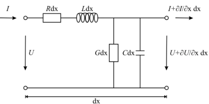
Fig. 1.Equivalent circuit of an infinitesimal section of a transverse electromagnetic (TEM) transmission-line.
inversion techniques: Pereira, 1997; Todoroff et al., 1998; Oswald, 2000; Heimovaara et al., 2004). A high spatial res-olution can be achieved by exploiting the full information content in the reflected electromagnetic signals of the sen-sor line (Lundstedt and He, 1996; Norgren and He, 1996). A new reconstruction algorithm has been developed which uses the full information of the TDR signals measured on one or both sides of the line. It is based on the telegraph equation for nonuniform transmission-lines and an optimiza-tion approach to reconstruct simultaneously one or two line parameters with high spatial resolution (Schlaeger, 2001). In comparison with other full wave inversion techniques (e.g. generic algorithms, Oswald, 2000) it needs clearly less com-putation expenditure. The optimization algorithm uses the conjugate-gradient-technique and fast simplex or complex methods.
Using laboratory tests it is shown that TDR reflection data from both sides of a buried flat-ribbon-cable sensor are suit-able for simultaneous reconstruction of capacitance and ef-fective conductance profiles. During an investigation of the transport of volatile organic compounds in medium grained sand (grain size 0.2 to 1 mm) the moisture profile under irrigation has been measured. In the steady state the vol-umetric water content varies along the vertically arranged transmission-line sensor of 71.7 cm between 0.5 and 44%. The changes in water content could be reconstructed with a high spatial accuracy and an average uncertainty of±2.3% compared to oven-drying measurements (Schlaeger et al., 2005)1.
To determine moisture profiles, appropriate TDR-devices (short pulse rise time, high sampling rate) and sensitive test-ing probes (well known electric parameters) are required. The mathematical model has to be chosen to describe the physical process during the measurement in a very accurate and computable way. The inversion algorithm starts with an initial guess of the electric parameter distribution. Us-ing this parameter distribution an associated TDR-signal can be calculated. The difference between the measurement and
1Schlaeger, S., H¨ubner, C., and Weber, K.: Moisture profile
de-termination with TDR, in preparation, 2005.
this simulation leads to a rough deformation-instruction for the given parameter distribution. During one optimization-step a new parameter distribution will be generated by de-forming the old distribution according to the deformation-instruction. In the next step the comparison between mea-surement and simulation leads to an improved deformation-instruction. The optimization will be continued until a mini-mum difference is reached. The resulting electric parameter distribution can be easily transformed into water content pro-files. The whole process is called Spatial-TDR.
The Soil Moisture Group (SMG) at the University of Karl-sruhe has tested this Spatial-TDR technology in many ap-plications. A monitoring system to measure the spatial soil water distribution on a full-scale levee model has been suc-cessfully implemented with transmission-lines up to 3 m and leads to significant specifications for drainage models (Scheuermann et al., 2001). The technology is also being used for flood warning systems, and snow moisture measure-ments (Becker et al., 2002; Stacheder et al., 2005), and for the determination of the water content of technical barriers in waste disposal sites (Becker et al., 2003).
2 Basic equations
The propagation of electromagnetic waves on insulated and non insulated transmission-lines can be described by the tele-graph equations. These equations were developed by Heavi-side in 1886. In this model the transmission-line is character-ized by four electrical parameters: the inductanceL, capaci-tanceC, series resistanceR, and shunt conductanceG. The equivalent electric circuit of an infinitesimal transmission-line section is given in Fig. 1. It is seen that the inductance and resistance are series elements that cause a voltage drop along the line, whereas the capacitance and conductance are shunt elements that provide a current path between the con-ductors.
From a circuit theory approach it is a simple matter to de-rive the telegraph equations that describe the variation of the voltageU (x, t )and the currentI (x, t )in the time along the transmission-line due to the influence of the electric param-eters of the line and the surrounding media. By applying Kirchhoff’s voltage and current laws to the equivalent circuit in Fig. 1, one obtains
∂
∂xU (x, t )= −R(x)I (x, t )−L(x) ∂
∂tI (x, t ) , (1) ∂
∂xI (x, t )= −G(x)U (x, t )−C(x) ∂
∂tU (x, t ) . (2)
UsuallyR andLare constant for the probe whereasC and
~ Zi
xa x1 x2
Ua L ,Ca a
L=L , C=C(x)0
R=0, G=G(x)
Fig. 2. Schematic representation of a sensitive transmission-line, situated betweenx1and x2, which is connected to a TDR-device on one side using a lossless uniform coaxial-cable with impedance Z=(La/Ca)0.5.
higher conductivity than sands. The capacitanceC is inti-mately connected with the permittivity and therefore the wa-ter content of the surrounding medium. The dewa-termination of the spatial distribution ofC(x)is the key component of the presented reconstruction of the soil water content.
The solution of Eqs. (1) and (2) describes the propagation in time and space of a supplied pulse to the whole measure-ment system. When the solution is restricted to one spatial point it represents a simulated measurement in this point. To calculate the solution initial and boundary conditions for the partial differential equations (PDE) are needed. It is also im-portant to consider the connection between TDR-device and testing probe. Usually they are connected with a lossless and uniform coaxial-cable (R=0,G=0,C=const, andL=const). Assume that there is no energy on the line at the beginning of the measurement. So the initial conditions can be set to
U (x, t )t≤0=0, I (x, t )t≤0=0, for allx . (3)
Than the Eqs. (1) and (2) can be transformed to one single PDE of second order
"
LC∂ 2
∂t2 +LG ∂ ∂t +
∂L∂x
L ∂ ∂x −
∂2 ∂x2
#
U (x, t )=0. (4) The derivative ofLhas to be considered in Eq. (4) because the inductance of the coaxial-cable and the testing probe are constant but may be different in general. The initial condi-tions (Eq. 3) can be transformed to
U (x, t )|t≤0=0, ∂
∂t U (x, t )|t≤0=0, for allx . (5)
To define the boundary conditions for the PDE (Eq. 4) the whole measurement configuration has to be considered. The sensitive transmission-line has to be inserted into the soil and must be connected to a TDR-device in order to excite an elec-tric pulse.
Figure 2 describes the experimental setup to receive the re-flection data from one side of the sensitive transmission-line. Therefore reflection measurements must be realized with an external currentFex=δ(x−x)a ·f (t ) atx=xa. The back-traveling wave is absorbed by the matched impedance Zi
Zi
xa x2
Ua
L ,Ca a
L=L , C=C(x)0
R=0, G=G(x)
~ ~
L ,Ce e
Zi
Ue
x1 xe
Fig. 3. The nonuniform transmission-line, situated between x1 andx2, is connected to two lossless uniform coaxial-cables with matched impedancesZiat their endpoints.
inside the TDR-device if it is equal to the impedanceZ of the coaxial-cable. This absorbing boundary condition for the lossless wave equation can be numerically implemented in the coaxial-cable using (Engquist and Majda, 1977):
∂ ∂x−
p LaCa
∂ ∂t
U (xa, t )=La ∂
∂tFex(xa, t ), t ≥0. (6)
The boundary conditions at the end of the sensitive line at
x=x2depends on its physical implementation. In case of an open-circuit the boundary condition will be
∂
∂tU (x2, t )=0, t ≥0. (7)
If there is a short-circuit atx=x2the boundary condition will
beU (x2, t )=0, fort≥0.
In order to reconstruct two parameters, two independent measurements are needed. Consequently, the problem is di-vided into two parts, the first dealing with an incident wave from the left and the second with an incident wave from the right side of the system under test.
Figure 3 describes the experimental setup to receive the re-flection data from both sides of the unknown material. There-fore two separate measurements must be realized with the ex-ternal currentFex1=δ(x−xa)·f (t )andFex2=δ(x−xe)·f (t ), respectively. U1(x, t )andU2(x, t )are the solutions of both separate forward problems. The setup of Fig. 3 can be trans-formed to the setup in Fig. 2 for each single-sided measure-ment using sensor switches (Becker and H¨ubner, 2003). In this case the solution ofU1(x, t )can be calculated according
toU (x, t )by using Eqs. (4)–(7). If there is a coaxial-cable permanently attached atx=xean absorbing boundary condi-tion has to be used instead of Eq. (7):
∂ ∂x +
p LeCe
∂ ∂t
U1(xe, t )=0, t ≥0. (8) For the other initial-boundary-value-problem (IBVP) forU2
with external current Fex2 the boundary conditions are ex-changed.
Before the reconstruction procedure can be started all nec-essary parameters (La, Ca, Le, Ce, L0)have to be measured
The inverse method presented in the next section is based on an iterative search for the electrical parameters of the nonuni-form transmission-line with the full wave solution of the di-rect problem. The solution of the line needs to be calculated repetitively. It is therefore important to use a technique for the determination of this solution that is computationally ef-ficient to guarantee low calculating time.
3 Optimization approach
The aim of the investigation is the determination of the un-known distribution ofC(x)with measurements of input and output data. The input dataf (t ), which describes the inci-dent pulse, can be easily determined from the reflection mea-surementsUa(xa, t )of the coaxial-cable betweenxaandx1
with an open-circuit atx=x1. The output dataλ(t )is the
re-flected signal based on the associated input signal at one side of the sensor line.
The cost functionJ (C)defines the squared difference (in
L2-norm) between the solution of the direct problem (Eqs. 4–
7) restricted tox=x1corresponding to one given parameter
distributionCand the measured reflectionsλ(t )atx=x1,
J (C)= kU (x1, t;C)−λ(t )k22= 2T Z
0
[U (x1, t;C)−λ(t )]2dt(9)
with T=τ (x1, x2), where τ (x1, x2) is the travel-time
be-tweenx1andx2. The cost function refers to the error in the
solution for single-sided incidence measurements. The con-cept of the method is to find the parameter distribution that minimize the cost functionalJ. If the problem has a solution the theoretical minimum ofJ is zero. One important reason for choosing theL2-norm is the possibility to derive exact expressions for the gradient ofJ.
3.1 Exact expression of the gradient of the cost function In the following section the gradient of the cost function will be determined for single-sided and double-sided reflection data, respectively. For one single measurement it is only pos-sible to calculate one parameter distributionC(x) or G(x)
while the other one is known (He et al., 1993). Assum-ing that the capacitance and conductance are connected by a transfer function then it is possible to calculate both pa-rameter distributions from one single reflection measurement using an empirical G(C)-relationship (Hakansson, 1997). This relationship depends not only on the water content but also on the electrolyte imbalance of the pore water. The determination of this relation may be very time intensive (Becker, 2004; Becker and Schlaeger, 2005). If both param-eter distributions are to be calculated simultaneously with-out thisG(C)-relationship, two independent measurements have to be carried out, e.g. double-sided reflection measure-ments (He et al., 1994). In the first case the gradient for
J (α)=J (C)orJ (α)=J (G), in the second case the gradient forJ (α)=J (C, G)is calculated. In both cases the gradient ∇J (α)can be calculated using the standard finite difference formulation forδα→0:
J (α+δα)−J (α)= hδα,∇J (α)i = ∞
Z
−∞
δα(x)· ∇J (α)(x)dx . (10)
3.1.1 Single-sided reflection data
In the case of only one single-sided reflection data-set it is reasonable to reconstruct the capacitance profileC(x)to de-termine the water content. Therefore the information about the gradient ∇J (C) has to be generated. According to Eq. (9), Eq. (10) can be transferred to
J (C+δC)−J (C) (11)
=
2T R
0
[U (x1, t;C+δC)−λ(t )]2−[U (x1, t;C)−λ(t )]2dt
=
2T R
0
U2(x1, t;C+δC)−U2(x1, t;C)
−2λ(t )[U (x1, t;C+δC)−U (x1, t;C)] dt
=
2T R
0
[U (x1, t;C+δC)+U (x1, t;C)]
| {z }
≈2U (x1,t;C)
·
[U (x1, t;C+δC)−U (x1, t;C)]
| {z }
=:δU (x1,t;C)
−2λ(t )·[U (x1, t;C+δC)−U (x1, t;C)]
| {z }
=:δU (x1,t;C)
dt
≈
2T R
0
2δU (x1, t;C)·[U (x1, t;C)−λ(t )]dt
=
2T R
0 ∞ R
−∞
δU (x, t;C)·2δ (x−x1)[U (x, t;C)−λ(t )] dx dt.
In Eq. (11) δ(x) represents the Dirac delta-function with ∫δ(x−x0)f (x)=f (x0)for all f. The difference between
two solutions according to a difference between C and
C+δC is defined byδU (C)=U (C+δC)−U (C). For small discrepancies inC the difference δU (C)is assumed to be also small andU (C+δC)+U (C)≈2U (C). To make further transformations of Eq. (11) the advantages of adjoint oper-ators will be used. Therefore a linear operatorLis defined analog to Eq. (4):
LU≡
"
LC∂ 2
∂t2 +LG ∂ ∂t +
∂L∂x
L ∂ ∂x −
∂2 ∂x2
#
U (12)
The definition of the adjoint operatorL∗is that he will fulfil the following equation for everyU (x, t )andV (x, t )
using the inner product
(U|V )=
2T Z 0 ∞ Z −∞
U (x, t )V (x, t ) dx dt . (14)
Now the PDE for the adjoint operatorL∗ has to be deter-mined. The left side of Eq. (13) can be transformed using Eqs. (12) and (14). Each of the double-integrals will be trans-formed to isolate U (x, t )using integration by parts in ev-ery addend. The auxiliary terms resulting from this isolation must be eliminated now, as the initial and boundary condi-tions forV are appropriate selected. The notationUtandUt t in the following equation is an abbreviation for the partial differential derivative∂U/∂tand∂2U/∂t2, respectively.
(LU|V ) (15)
= 2T R 0 ∞ R −∞
LCUt tV dxdt + 2T R 0 ∞ R −∞
LGUtV dxdt
+ 2T R 0 ∞ R −∞ Lx
LUxV dxdt− 2T R 0 ∞ R −∞
UxxV dxdt
= ∞ R
−∞
LC [UtV]tt==02T − [U Vt]tt==20T + 2T R
0
U Vt tdt ! dx + ∞ R −∞
LG [U V]tt==20T −
2T R
0 U Vtdt
! dx + 2T R 0
[ULx
LV] x=∞ x=−∞−
∞ R −∞ U Lx L
xV dx− ∞ R
−∞ ULx
LVxdx ! dt − 2T R 0
[UxV]xx=∞=−∞− [U Vx]xx=∞=−∞+ ∞ R
−∞
U Vxxdx ! dt #1 = 2T R 0 ∞ R −∞
LCVt tU dxdt− 2T R 0 ∞ R −∞
LGVtU dxdt
− 2T R 0 ∞ R −∞ Lx
LVxU dxdt− 2T R 0 ∞ R −∞
VxxU dxdt
#2
= U|L∗V
To make sure that transformation #1 in Eq. (15) is correct the initial and boundary conditions forV (x, t )have to be set as follows
V (x,2T )=0, ∂
∂tV (x,2T )=0,−∞< x <∞, (16) V (−∞, t )=0, ∂
∂tV (∞, t )=0,0≤t≤2T . (17)
The initial condition results to a backward propagation in time from 2T to zero. When the operatorL∗is defined by
L∗V ≡
"
LC∂ 2
∂t2 −LG ∂ ∂t −
∂L∂x
L ∂ ∂x − ∂2 ∂x2 # V (18)
then equivalence #2 in Eq. (15) will also be fulfilled. Now the adjoint operatorL∗that accomplishes Eq. (13) is found with its corresponding PDE (Eq. 18) and initial and boundary conditions (Eqs. 16–17). The solution V of this PDE can only be different from zero if a non vanishing right side is assigned toL∗V. Looking back to Eq. (11) one can equate
L∗V =2δ (x−x1)[U (x, t;α)−λ(t )] (19) to continue the transformations of Eq. (11) and use the prop-erty ofL∗ being the adjoint operator toLaccording to the inner product (Eq. 14).
J (C+δC)−J (C) (20)
= 2T R 0 ∞ R −∞
δU· L∗Vdx dt
= 2T R 0 ∞ R −∞
(LδU )·V dx dt
= 2T R 0 ∞ R −∞ V h
LδCUt t +LCδUt t+LGδUt+LLxδUx−δUxx i dx dt = ∞ R −∞ δC 2T R 0
V LUt tdt dx
+ 2T Z 0 ∞ Z −∞ V
LCδUt t+LGδUt + Lx
LδUx−δUxx
dxdt
| {z }
→0f orkδCk→0
From Eqs. (20) and (10) it follows that
∇J (C)=
2T Z
0 LV ∂
2
∂t2U dt = − 2T Z 0 L∂ ∂tV ∂
∂tU dt. (21)
This gradient can be calculated by solving two IBVP: One forward problem for the direct wave (Eqs. 4–7) and one back-ward problem for the adjoint wave (Eqs. 16–19).
3.1.2 Double-sided reflection data
For the simultaneous reconstruction ofC(x)andG(x)it is necessary to take two independent measurements. As shown in the previous section one choice will be the two reflection measurements from both sides of the sensor:
λ1(t )=Ua(x1, t ), λ2(t )=Ue(x2, t ) (22)
It is also necessary to choose another cost function in order to minimize the error between the simulation and the mea-surements simultaneously. ChoosingJ (α)=J (C, G)as
J (α)=
2 X
i=1 2T Z
0
Initial parameter distributiona(0)
P(0) J( =-Ñ a )(0)
k=0 k=k+1
Iterative search forg(k)with g =(k) a +g(k) (k)
min J( P )
g
New parameter distribution P a(k+1)=a +g(k) (k) (k)
||a(k+1)-a || < e(k)
Final parameter distribution a(k+1)
Yes
No
||Ñ aJ( (k+1))||2 ||Ñ aJ( (k)) ||2 P(k+1) J( (k+1)) P(k)
=-Ñ a + New search direction Initial search direction
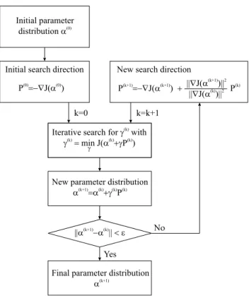
Fig. 4. Flow chart of the Fletcher-Reeves conjugate gradient method.
The determination of the two gradients is very similar to the transformations above. It leads to the same adjoint PDE for
L∗as in Eq. (18). But two different backward problems have to be calculated according to the two different forward solu-tionsU1andU2. The right sides of the adjoint problems are
given by
L∗Vi =2δ (x−xi)[Ui(x, t;α)−λi(t )], i=1,2 (24) and the initial and boundary conditions have to be chosen to fulfil
Vi(x,2T )=0, ∂
∂tVi(x,2T )=0,−∞<x<∞, i=1,2, (25) Vi(−∞, t )=0,
∂
∂tVi(∞, t )=0,0≤t≤2T , i=1,2. (26)
For each givenα=(C(x), G(x))one can solve the forward problems forU1(x, t )andU2(x, t )and the backward prob-lems forV1(x, t )andV2(x, t )and calculate the gradients of
J (α)with respect toCandG, respectively:
∇CJ (α)= −
2 X
i=1 2T Z
0 L∂
∂tVi ∂
∂tUidt (27)
∇GJ (α)=
2 X
i=1 2T Z
0 LVi
∂
∂tUidt (28)
3.2 Reconstruction of the parameter distribution
To determine the distribution ofα=C(x)a conjugate gradi-ent (cg) method is appropriate if the gradigradi-ent of the func-tion to be minimized can be calculated explicitly and very easily. Starting with a parameter distribution α(0) the first search direction is given by the direction of steepest decent
P(0)=−∇J (α(0)). The next parameter distribution can be calculated by
α(k+1)=α(k)+γ(k)P(k) (29)
whereγ(k)is the optimal step-size to minimize the cost func-tion based on the former parameter distribufunc-tionα(k)and the search-directionP(k):
γ(k)=min γ J
α(k)+γ ·P(k)
. (30)
The main effort of computation in this minimization is due to the large number of cost function analysis. Therefore an effective numerical algorithm concerning minimum function calls is the core of a fast reconstruction algorithm. In com-parison to conventional cg-methods the following search di-rectionP(k+1)is not only the direction of steepest decent at
α(k+1)but also a combination of former search-directions.
P(k+1)= −∇Jα(k+1)+
∇J α(k+1)2
2
∇J α(k)2
2
·P(k) (31)
This leads to a faster convergence and less calculation effort. The cg-method was chosen according to Fletcher and Reeves (1964) – similar results were carried out by using the cg-method according to Polak and Ribi`ere (1969).
During simultaneous reconstruction ofC(x)andG(x)the minimum search in Eq. (30) will be extended to a two-dimensional search:
γ(k), η(k)
=min γ ,η J
C(k)+γ ·PC(k), G(k)+η·PG(k)
(32)
Especially in this two-dimensional search the choice of an algorithm with as few function calls as possible is of cru-cial importance. The simplex method developed by Nelder and Mead (1965) and the complex method by Box (1965) lead to fast optimization algorithms even in the simultane-ous reconstruction of two parameter functions. At one- and two-parameter optimization the conjugate gradient algorithm terminates if there is no significant change in the value of two consecutive cost functions. Figure 4 shows the flow chart of the preferred cg-method.
Fig. 5.Insulated flat-ribbon-cable (short section with bare conduc-tors to visualize the geometry and the electrical connection of the cable) with a sensor switch between coaxial cable and flat-ribbon-cable.
Table 1.Cable parameters for the sensor cable in Fig. 5.
Circuit element C1 C2 C3 L0
(pF/m) (pF/m) (pF/m) (nH/m)
Measured value 3.4 323 14.8 756
Calculate value 4.0 308 13.7 785
4 Determination of the water content
The capacitance profileC(x)describes the electrical proper-ties of the whole medium around the conductors of the sen-sitive transmission-line. But strictly speaking, the capaci-tance at any point of the profile is not independent on the frequency. For simplification, we assume that there may be a constant value forCfor the used TDR frequency range de-pending on feeding cable properties and length. If the sensor is not insulatedC(x)can be easily transformed into the rel-ative permittivity of the mediumεm(x)=L0c02C(x), where L0specifies the inductance of the sensor andc0the speed of
light in vacuum. If the sensor is insulated with some dielec-tric material the total capacitanceC(x)represents the com-bination of insulation and soil. Therefore a sensor specific transformation fromC to the relative permittivity ε of the soil is necessary.
The flat-ribbon-cable used for many applications of the SMG is shown in Fig. 5. It has been developed and patented by the Institute of Meteorology and Climate Research at the Forschungszentrum Karlsruhe (Brandelik et al., 1998). The cable consists of three flat copper wires covered with polyethylene. The electrical field is concentrated around the conductors and defines the sensitive area of 3 to 5 cm around the cable depending on the permittivity. The electric prop-erties of the flat-ribbon-cable used in this work can be
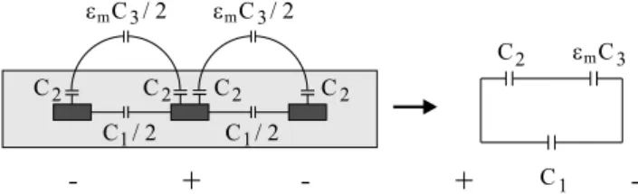
mea-Fig. 6. Capacitance model of the insulated flat-ribbon-cable from Fig. 5.
sured and calculated (cf. Fig. 6 and Table 1).
According to the equivalent circuit of Fig. 6 the total ca-pacitanceCcan be expressed by three capacitancesC1,C2,
andεmC3and can be transformed into a direct relation
be-tween the relative permittivityεmof the surrounding soil and the total capacitance:
C=C1+ C2εmC3
C2+εmC3
(33) The three unknown capacitances C1, C2, and C3 were de-rived from calibration measurements of three different ma-terials with well known dielectric properties, e.g. air, oil, and water. The inductance was determined by measuring the wave impedance with a variable resistor at the end of the ca-ble adjusted for minimum reflection. The values for the caca-ble of Fig. 5 are given below (H¨ubner, 1999).
The permittivity of the soil can now be transformed to the volumetric water content by standard transformations for ar-bitrary soils (e.g. Topp et al., 1980) or soil specific calibration functions determined from laboratory test series. The accu-racy of the water content distribution depends highly on the accuracy of this transformation. The deviation due to insuffi-cient knowledge of the material can easily exceed the errors of the reconstruction of the capacitance profileC(x).
The total conductanceG(x)describes the conductivity of the material between the copper wires, i.e. the system of polyethylene insulation and the surrounding material. The determination of the water content distribution of the sur-rounding material does not require the knowledge of the con-ductivity distribution of the material, but it cannot be ne-glected during the reconstruction ofC(x).
5 Numerical results
Table 2.Electrical properties of the test materials to represent loss-less and lossy material.
Position (m)
0.0–0.3 0.3–1.3 1.3–1.7 1.7–2.0
Lossless C (pF/m) 20 40 80 20
G (mS/m) 0 0 0 0
Lossy C (pF/m) 20 40 80 20
G (mS/m) 0 4 8 0
changes of this synthetic example natural soil profiles show smooth transients in the water content (related to the chosen spatial discretization step).
These parameter distributions lead to left- and right-sided reflection data for the lossless and lossy material (H¨ubner et al., 2005), see Fig. 7.
The initial capacitanceC0=τ2(x1, x2)/(L0(x2−x1)2)can
be easily determined by simple travel-time measurements along the cable sensor (Heimovaara and Bouten, 1990). To ensure the invariance of this sensor travel-time during the conjugate gradient algorithm one has find a constant shiftCγ for every givenγ during the optimization to fulfil
p
C0(x2−x1)=
Z x2
x1 q
C(x)+γ PC+Cγdx (34) This shift correction guarantees that all determined capac-itance profiles lead to the same total travel-time along the cable sensor. It means that the mean moisture content re-mains invariant during the optimization. Therefore the sin-gle roundtrip travel-timeτ (x1, x2)has to be determined as accurate as possible. Equation (29) has to be modified to get the advanced consecutive capacitance profile in the cg-algorithm:
C(k+1) =C(k)+γ(k)P(k)+Cγ(k) (35) with
γ(k)=min γ J
C(k)+γ ·P(k)+Cγ
. (36)
5.1 One-parameter reconstruction
Compared to lossy materials the reconstruction of the true capacitance profile in lossless soil (G(x)=0)is rather sim-ple. Only one unknown parameter distributionC(x)has to be determined. Therefore one single reflection measurement is sufficient to derive the final capacitance profile.
To calculate the wave propagation the cable sensor is sepa-rated into 400 equally spaced sections of 5 mm. For this dis-cretization the single-sided reconstruction algorithm needs about 15 min on a standard PC to calculate 20 iteration steps. The similar reconstruction using right-sided reflection data leads to comparable results.
0 5 10 15 20
0 0.5 1
travel time [ ns ]
reflection data [ − ]
lossless medium (left−sided reflection) lossless medium (right−sided reflection)
0 5 10 15 20
0 0.5 1
travel time [ ns ]
reflection data [ − ]
lossy medium (left−sided reflection) lossy medium (right−sided reflection)
Fig. 7.Left- and right-sided reflection data for the lossless (above) and lossy (below) soil profile, both with main reflections at 22.3 ns as a result of an open-circuit at the end of the cable sensor.
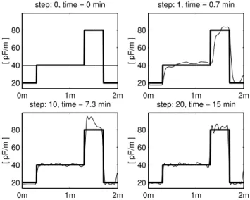
Figure 8 shows several intermediate results during the con-jugate gradient optimization. The search direction leads to a good approximation of the capacitance profile very fast. Af-ter the first iAf-teration the main features are mapped very well. The following iterations lead to smaller corrections of rather fine structures.
In the case of lossy material with an unknown effective conductance profileG(x)a first approach is to reconstruct
C(x)using single-sided reflection data and assumeG(x)to be equal to zero over the whole area. Figure 9 show the re-sults of this reconstruction. The capacitance is overestimated due to the effect of the non vanishing conductivity. Further-more the optimization stops after three iteration steps, be-cause the calculated search direction could not improve the value of the cost function (Eq. 9).
This distortion is reduced if the mean value of the conduc-tance will be used which can also be determined from the time domain reflection. A mean value ofG(x) = 4 mS/m was chosen to estimate the effect of the conductivity. Fig-ure 10 shows the reconstruction of the capacitance using this assumption.
The results of the capacitance reconstruction presented in Figs. 9 and 10, do not satisfy the expectations on a reliable solution of the soil moisture determination. To get better re-sults it is necessary to use additional information to recon-struct the capacitanceC(x)and the conductanceG(x) simul-taneously.
5.2 Two-parameter reconstruction
0m 1m 2m 20
40 60 80
step: 0, time = 0 min
[ pF/m ]
0m 1m 2m
20 40 60 80
step: 1, time = 0.7 min
[ pF/m ]
0m 1m 2m
20 40 60 80
step: 10, time = 7.3 min
[ pF/m ]
0m 1m 2m
20 40 60 80
step: 20, time = 15 min
[ pF/m ]
Fig. 8. Capacitance profiles C(x) during the reconstruction from left-sided reflection data (thin line) for lossless material (G(x)≡0 mS/m) compared to the true profile (bold line).
0m 1m 2m
20 40 60 80 100
step: 0, time = 0 min
[ pF/m ]
0m 1m 2m
20 40 60 80 100
step: 3, time = 10.4 min
[ pF/m ]
Fig. 9. Capacitance profilesC(x)during the reconstruction from left-sided reflection data (thin line) for lossy material (wrong as-sumption ofG(x)≡0 mS/m during reconstruction) compared to the true profile (bold line).
sides of the cable sensor are used. The minimization of Eq. (23) requires the determination of the solution of two in-dependent IBVP. In addition to this duplication of the calcu-lation effort the conjugate gradient method is more complex. To find the optimal step sizes for each search direction a two-dimensional search has to be treated. This causes a much larger calculation time for every iteration step. To keep the total calculation time acceptable, the terminating condition to exit the conjugate gradient method has to be less strict.
Figure 11 shows the result of the optimization during sev-eral iteration steps. The algorithm terminates after 8 iteration steps although the approximation to the true profile is not as good as for the single-sided reflection data. But in addition to the capacitance profile the algorithm leads to a conductivity profile (see Fig. 12).
This conductivity profile represents the total conductance of the composite of insulation and surrounding soil. A trans-formation fromG(x)to the soil conductivityσ (x)is not re-quired because it gives no further information to the water content. But further investigations may close this gap.
0m 1m 2m
20 40 60 80 100
step: 0, time = 0 min
[ pF/m ]
0m 1m 2m
20 40 60 80 100
step: 1, time = 1.4 min
[ pF/m ]
0m 1m 2m
20 40 60 80 100
step: 10, time = 12.6 min
[ pF/m ]
0m 1m 2m
20 40 60 80 100
step: 20, time = 24.1 min
[ pF/m ]
Fig. 10. Capacitance profilesC(x)during the reconstruction from left-sided reflection data (thin line) for lossy material (assumption of constantG(x)≡4 mS/m during reconstruction) compared to the true profile (bold line).
0m 1m 2m
20 40 60 80
step: 0, time = 0 min
[ pF/m ]
0m 1m 2m
20 40 60 80
step: 1, time = 17.4 min
[ pF/m ]
0m 1m 2m
20 40 60 80
step: 4, time = 61.4 min
[ pF/m ]
0m 1m 2m
20 40 60 80
step: 8, time = 118.1 min
[ pF/m ]
Fig. 11. Capacitance profilesC(x)during the reconstruction from double-sided reflection data (thin line) for lossy material compared to the true profile (bold line).
Finally the iteration speed and the total calculation time of the presented numerical examples were investigated. The results are presented in Fig. 13.
0m 1m 2m 0
5 10
step: 0, time = 0 min
[ mS/m ]
0m 1m 2m
0 5 10
step: 1, time = 17.4 min
[ mS/m ]
0m 1m 2m
0 5 10
step: 4, time = 61.4 min
[ mS/m ]
0m 1m 2m
0 5 10
step: 8, time = 118.1 min
[ mS/m ]
Fig. 12.Conductance profilesG(x)during the reconstruction from double-sided reflection data (thin line) for lossy material compared to the true profile (bold line).
in mind the logarithmic scale of the y-axis in the upper dia-gram of Fig. 13).
The calculation effort stays constant in every iteration step and is nearly equal for the compared one-parameter recon-structions. It increases rapidly when using the two-parameter reconstruction due to the two-dimensional step size opti-mization. But this calculation time is almost fast enough for many applications and surely contributes to the further spreading of this method.
The software for this reconstruction algorithm has been developed using MATLAB®. It has been employed to many applications of the SMG for different transmission lines be-tween 0.3 and 20 m in length. Progress is intended to con-tinue and the relevant software can be available shortly.
6 Conclusions
A fast inversion technique is presented that derives capaci-tance profiles in high spatial resolution from single TDR re-flection measurements. The algorithm is based on an opti-mization approach to minimize the difference between the measurement and simulated TDR reflection data depending on a given parameter distribution. The optimization is done with conjugate gradients due to the fact that the gradient can be calculated explicitly. This gradient can be deter-mined very fast by solving only two initial-boundary-value-problems instead of several hundred when using standard Hessian matrix inversion techniques. The algorithm iterates very fast and leads to reliable soil moisture profiles which can be derived from the capacitance profiles by standard transfor-mations.
0 5 10 15 20 25 30 35 40
10−12 10−10 10−8
Number of iterations
cost functional [ − ]
1−parameter: lossless (G=0 mS/m) 1−parameter: lossy (guess G=0 mS/m) 1−parameter: lossy (guess G=4 mS/m) 2−parameter: lossy
0 5 10 15 20 25 30 35 40
0 50 100
Number of iterations
Total time [ min ]
1−parameter: lossless (G=0 mS/m) 1−parameter: lossy (guess G=0 mS/m) 1−parameter: lossy (guess G=4 mS/m) 2−parameter: lossy
Fig. 13.Results of the cost function (above) and the total calculation time (below) after each iteration step of the cg-method.
The results of this study of this new inversion technique for time domain reflectometry data show that single-sided reflection data are capable for the reconstruction of the soil moisture profile for lossless (or low-loss) soils. The full in-formation content of one single travel-time roundtrip can be used to determine the capacitance profileC(x)and the as-sociated volumetric water content on a standard PC in rea-sonable time. In the case of lossy soils more information is required. The knowledge of the conductance profile G(x)
or an experimental determined relationship between capaci-tance and conduccapaci-tance for the used sensor and soil can im-prove the determination of moisture profiles using only one single measurement. If none of this knowledge is available one more independent reflection measurement is required.
The presented inversion technique is also suitable for the simultaneous reconstruction of capacitance and conductance profile using double-sided reflection data. The resulting profiles are more reliable than single-sided reconstructions with standard assumptions to the conductivity (e.g. constant conductivity distributions). The simultaneous reconstruction of C(x) and G(x) and the associated volumetric water content can also be done within a reasonable time.
Edited by: N. Romano
References
Becker, R.: Spatial time domain reflectometry for monitoring tran-sient soil moisture profiles, Ph.D. thesis, Institut f¨ur Wasser und Gew¨asserentwicklung – Bereich Wasserwirtschaft und Kul-turtechnik, Mitteilungen Heft 228, Universit¨at Karlsruhe, 2004. Becker, R. and H¨ubner, C.: Messger¨ateentwicklungen der Soil
Feuchtemessung in Forschung und Praxis”, Karlsruhe, Germany, 3–4 July 2003.
Becker, R. and Schlaeger, S.: Spatial time domain reflectometry with rod probes, Proceedings of the 6th Conference on “Electro-magnetic Wave Interaction with Water and Moist Substances”, ISEMA 2005, Weimar, Germany, 20 May–1 June 2005. Becker, R., Bieberstein, A., H¨ubner, C., N¨uesch, R., Sch¨adel, W.,
Scheuermann, A., Schlaeger, S., and Schuhmann, R.: Nonde-structive in situ and online measurements of soilphysical param-eters, in Soil and Rock America 2003, 12th Panamerican Confer-ence on Soil Mechanics and Geotechnical Engineering, 39th US Rock Mechanics Symposium, Cambridge, 22–26 June, 2003. Becker, R., Brandelik, A., H¨ubner, C., Sch¨adel, W., Scheuermann,
A., and Schlaeger, S.: Soil and snow moisture measurement sys-tem with subsurface transmission lines for remote sensing and environmental applications – Results of the Soil Moisture Group of the University of Karlsruhe, in Proceedings of the Open Sym-posium on Propagation and Remote Sensing, URSI Commission-F, Garmisch-Partenkirchen, Germany, 12–14 February 2002. Birchak, J. R., Gardner, C. G., Hipp, M. E., and Victor, J. M.: High
dielectric constant microwave probes for sensing soil moisture, Proceedings of the IEEE, 62, 93–98, 1974.
Brandelik, A., Huebner, C., and Schuhmann, R.: Moisture sen-sor for large area layers (German patent no. 4432687, European patent no. 0804724, US patent no. 5942904), 16 June 1998. Box, M. J.: A new method of constraint optimization and a
com-parison with other methods, The Computer Journal, 8, 43–52, 1965.
Chambarel, A., Ferry, E., Chanzy, A., Laurent, J.-P., Todoroff, P., and Ferrari: P.: TDR signal modeling using the electric line approach: model validation and signal inversion to retrieve soil moisture profile, TDR 2001, Evanston, Illinois, 5–7 September 2001.
Dasberg, S. and Dalton, F. N.: Time domain reflectometry field measurements of soil water content and electrical conductivity, Soil Sci. Soc. Am. J., 49, 293–297, 1985.
Engquist, B. and Majda, A.: Absorbing boundary conditions for the numerical simulation of waves, Mathematics of Computa-tion, 31, 629–651, 1997.
Feng, W., Lin, C. P., Deschamps, R. J., and Drnevic, V. P.: Theo-retical model of a multisection time domain reflectometry mea-surement system, Water Resources Research, 35, 8, 2321–2331, 1999.
Fletcher, R. and Reeves, C. M.: Function minimization by conju-gate gradients, The Computer Journal, 7, 149–154, 1964. Hakansson, G: Reconstruction of soil moisture profile using
time-domain reflectometer measurements, Master thesis, Royal In-stitute of Technology, Department of Electromagnetic Theory, Stockholm, 1997.
He, S., Kabanikhin, S. I., Romanov, V. G., and Str¨om, S.: Analy-sis of the Green’s function approach to one-dimensional inverse problems, Part I: One parameter reconstruction, J. Math. Phys., 34, 5724–5746, 1993.
He, S., Romanov, V. G., and Str¨om, S.: Analysis of the Green’s function approach to one-dimensional inverse problems, Part II: Simultaneous reconstruction of two parameters, J. Math. Phys., 35, 2315–2335, 1994.
Heimovaara, T. J. and Bouten, W.: A computer-controlled 36-channel time domain reflectometry system for monitoring soil
water content, Water Resources Research, 26, 2311–2316, 1990. Heimovaara, T. J., Huismann, J. A., Vrugt, J. A., and Bouten, W.: Obtaining the spatial distribution of water content along a TDR probe using the SCEM-UA Bayesian inverse modelling scheme, Vadose Zone Journal, 3, 1128–1145, 2004.
Hook, W. R., Livingston, N. J., Sun, Z. J., and Hook, P. B.: Remote diode shorting improves measurement of soil water by time do-main reflectometry, Soil Sci. Soc. Am. J., 56, 1384–1391, 1992. H¨ubner, C.: Entwicklung hochfrequenter Messverfahren zur Boden- und Schneefeuchtebestimmung, Ph.D. thesis, 199 pp., Forschungszentrum Karlsruhe, Institute for Meteorology and Climate Research, Scientific Report FZKA 6329, Karlsruhe, 1999.
H¨ubner, C., Schlaeger, S., Becker, R., Scheuermann, A., Brandelik, A., Sch¨adel, W., and Schuhmann, R.: Advanced measurement methods in time domain reflectometry for soil moisture determi-nation, in: Electromagnetic Aquametry, edited by: Kupfer, K., Springer, Berlin, Heidelberg, New York, 2005.
Lundstedt, J. and He, S.: A time-domain optimization technique for the simultaneous reconstruction of the characteristic impedance, resistance and conductance of a transmission line, J. Electro-magn. Waves and Appl., 10, 581–602, 1996.
Nelder, J. A. and Mead, R.: A simplex method for function mini-mization, The Computer Journal, 7, 308–313, 1965.
Norgren, M. and He, S.: An Optimization approach for the frequency-domain inverse problem for a nonuniform LCRG transmission line, IEEE Transaction on Microwave Theory and Technique, 44, 1503–1507, 1996.
Oswald, B.: Full wave solution of inverse electromagnetic prob-lems, Ph.D. thesis Swiss Federal Institute of Technology, Z¨urich, 2000.
Pereira, D. S.: D´eveloppement d’une nouvelle m´ethode de d´etermination des profils de teneur en eau dans les sols par in-version d’un signal TDR, Ph.D. thesis, Lab. D’Etude des Transf. En Hydrol. Et Environ., (LTHE), Univ. Joseph Fourier-Grenoble I, Grenoble, France, 1997.
Polak, E. and Ribi`ere, G.: Note sur la convergence de methodes de directions conjugees, Revue Franc¸aise d’Informatique et de Recherche Operationelle, Serie Rouge, 3, 35–43, 1969. Robinson, D. A., Jones, S. B., Wraith, J. M., Or, D., and
Fried-man, S. P.: A review of advances in dielectric and electrical con-ductivity measurement in soils using time domain reflectometry, Vadose Zone Journal, 2, 444–475, 2003.
Scheuermann, A., Schlaeger, S., H¨ubner, C., Brandelik, A., and Brauns, J.: Monitoring of the spatial soil water distribution on a full-scale dike model, in Proceedings of the Fourth International Conference on Electromagnetic Wave Interaction with Water and Moist Substances, Weimar, MFPA, 343–350, 2001.
Schlaeger, S.: Inversion von TDR-Messungen zur Rekonstruktion r¨aumlich verteilter bodenphysikalischer Parameter, Ph.D. the-sis, Ver¨offentlichungen des Institutes f¨ur Bodenmechanik und Felsmechanik der Universit¨at Fridericiana in Karlsruhe, vol. 156, 189 pp., Karlsruhe, Germany, 2002.
Todoroff, P., Lorion, R., and Lan Sun Luk, J. D.: L’utilisation des algorithmes g´en´etiques pour l’identification de profil hydriques de sol a partir de courbes r´eflectrom´etriques, C.R. Acad. Sci. Ser. IIa, Sci. Terre Planetes, 327, 607–610, 1998.
Todoroff, P. and Lan Sun Luk, J. D.: Calculation of in situ soil water content profiles from TDR signal traces, Measurement Science and Technology, 12, 27–36, 2001.
Topp, G. C. and Davis, J. L.: Measurement of soil water content using time-domain reflectometry (TDR): A field evaluation, Soil Sci. Soc. Am. J., 49, 19–24, 1985.
Topp, G. C., Davis, J. L., and Annan, A. P.: Electromagnetic deter-mination of soil water content. Measurements in coaxial trans-mission lines, Water Resources Research, 16, 574–582, 1980.
Topp, G. C., Davis, J. L., and Annan, A. P.: Electromagnetic de-termination of soil water content using TDR: I Applications to wetting fronts and steep gradients, Soil Sci. Soc. Am. J., 46, 672– 678, 1982a.
Topp, G. C., Davis, J. L., and Annan, A. P.: Electromagnetic de-termination of soil water content using TDR: II Evaluation of installation and configuration of parallel transmission lines, Soil Sci. Soc. Am. J., 46, 678–684, 1982b.