Light Field Imaging Based Accurate Image
Specular Highlight Removal
Haoqian Wang1, Chenxue Xu1, Xingzheng Wang1*, Yongbing Zhang1, Bo Peng2
1Shenzhen Key Laboratory of Broadband Network & Multimedia, Graduate School at Shenzhen, Tsinghua University, Shenzhen, China,2Department of Software Engineering, Southwest Jiaotong University, Chengdu, China
Abstract
Specular reflection removal is indispensable to many computer vision tasks. However, most existing methods fail or degrade in complex real scenarios for their individual drawbacks. Benefiting from the light field imaging technology, this paper proposes a novel and accurate approach to remove specularity and improve image quality. We first capture images with specularity by the light field camera (Lytro ILLUM). After accurately estimating the image depth, a simple and concise threshold strategy is adopted to cluster the specular pixels into “unsaturated”and“saturated”category. Finally, a color variance analysis of multiple views and a local color refinement are individually conducted on the two categories to recover dif-fuse color information. Experimental evaluation by comparison with existed methods based on our light field dataset together with Stanford light field archive verifies the effectiveness of our proposed algorithm.
Introduction
Image specular reflection has long been problematic in computer vision tasks [1]. They appear as surface features, but in fact they are artifacts caused by illumination changes from different viewing angles [2]. Most algorithms in computer vision such as segmentation [3] (which typi-cally assumes the intensity changes uniformly or smoothly across a surface), or stereo matching [4], recognition [5–9], image analysis [10–14]and tracking [15] (they attempt to match images taken from various conditions, i.e., viewing angle, illumination or distance, so they need a con-sistent surface of an object in different images) ignore the presence of specular pixels and work under the assumption of perfect diffuse surfaces. However, a vast majority of materials contain both diffuse and specular reflections in the real world. As a result, processing images with spec-ular reflections using these algorithms can lead to significant inaccuracies [1,16].
In recent years, various techniques try to handle the problem of specular reflections. Based on the number of input images, these methods could be divided into two main categories: mul-tiple-image based and single-image based [1]. Mulmul-tiple-image based approaches involve an image sequence of the same scene taken either from different viewpoints [16], with different illumination [17] or utilizing an additional polarizing filter. Nevertheless, obtaining such an
a11111
OPEN ACCESS
Citation:Wang H, Xu C, Wang X, Zhang Y, Peng B (2016) Light Field Imaging Based Accurate Image Specular Highlight Removal. PLoS ONE 11(6): e0156173. doi:10.1371/journal.pone.0156173
Editor:You Yang, Huazhong University of Science and Technology, CHINA
Received:November 22, 2015
Accepted:May 10, 2016
Published:June 2, 2016
Copyright:© 2016 Wang et al. This is an open access article distributed under the terms of the
Creative Commons Attribution License, which permits unrestricted use, distribution, and reproduction in any medium, provided the original author and source are credited.
Data Availability Statement:All relevant data are available on Figshare (https://figshare.com/articles/ Light_Field_Imaging_Based_Accurate_Image_ Specular_Highlight_Removal/3384112).
image sequence is difficult, time-consuming or even impractical [18–23]. Single-image based approaches require color or texture analysis [23–25]. They achieve acceptable results in some images, but they are unstable when the analyzed image has complicated textures and extreme specularities [23].
Benefiting from computational photography [26] and light field (LF) imaging technologies [27,28], we propose an accurate and novel framework that uses LF cameras to remove specu-larity. A handheld LF camera mounts an array of microlens in front of the sensor, which could record the full 4D rays to describe the scene, so one can refocus the image after a passive sin-gle–shot capture and shift viewpoints within sub-apertures of the main lens. With a LF camera to capture multiple views of the scene in a LF image, we could avoid the implementation com-plexity of conventional multiple-image based specular removal methods. In our algorithm, by exploiting the LF image to extract perspectives and modify focus, specular pixels could be detected and classified into“unsaturated”and“saturated”types, then replaced by their diffuse color via a color variance analysis of multiple views and a local color refinement. Thus, specular reflections could be substantially eliminated while the color consistency is well maintained in the rest part of the image. Moreover, the proposed algorithm can handle images which contain non-chromatic (i.e. R = G = B) and saturated specular pixels. It’s tested on various databases: the indoor and outdoor LF images taken by our Lytro ILLUM camera and the LF images from the Stanford light field archive [29]. It’s compared against three competitive methods: Tan et al. [24], Shen et al. [30] and Yang et al. [23].
The remainder of this paper is organized as follows. Section II introduces a brief review of the previous work related to highlight removal. Section III presents the basic knowledge of light field data, physical properties of reflection and dichromatic reflection model. In Section IV, we elaborate our algorithm in detail. We provide experimental results for real images in Section V. Lastly, concluded remarks are made in Section VI.
Related work
Multiple-image based highlight removal methods
This category utilizes a sequence of images, taking advantage of the different behaviors which these two reflections possess under specific conditions. Nayar et al. [31] achieved separation by incorporating polarization and color to obtain constraints on reflection components of each scene point, so the algorithm could work for textured surfaces. Unfortunately, obvious errors occur in the specular component on region boundaries due to chromatic aberration effects and mis-registration between polarization images. Later, Sato and Ikeuchi [32] examined a series of color images in a four-dimensional space and constructed a temporal-color space, which could describe the color change under the illumination densely varying with time. Lin and Shum [33] also changed the light direction to produce two color photometric images and estimated specu-lar intensity from a linear model of surface reflectance, but when the surface color is simispecu-lar to the illumination color, some specularity would be lost. In addition to that, light sources of the real world are usually fixed, especially in the outdoor scenes where light is not always controlla-ble. These approaches have produced good results, but the need for polarization or changing light direction greatly restricts their applicability.
Consequently, a number of researchers tried to fix the illumination and vary viewpoints to make the decomposition. Their basic ideas mainly utilize the fact that when viewing from vari-ous directions, the color of diffuse reflection doesn’t change, but that of specular reflection or a mixture of the two does. Using multi-view color images, Lee and Bajcsy [34] proposed a spec-tral differencing algorithm to seek specularities. Later, Lin et al. [16] integrated this work with multi-baseline stereo to yield good separation; nevertheless, large baseline would lead to severe
and analysis, decision to publish, or preparation of the manuscript.
occlusions which might be mislabeled as specularity. Criminisi [35] looked into the Epipolar plane image (EPI) strips to detect specular pixels, but some artifacts showed up because of incorrect EPI-strip selection. Furthermore, configuring and adjusting the required cameramay not be easy.
Single-image based highlight removal methods
In the last few years, considerable effort has been devoted to this category. For multi-colored images, many single-image based methods involve explicit color segmentation [36,37] which is often non-robust for complex textures and specularities, or require user assistance for high-light detection [2]. Shafer [38], who introduced the dichromatic reflection model, proposed a method based on a simple knowledge: by spectral projection in color space, points on a single surface must lie within a parallelogram and be bounded by diffuse and specular colors. Klinker [37] classified color pixels as matte (diffuse reflection only), highlight (specular and diffuse reflections) and clipped (highlight that exceeds the camera dynamic range), then produced a skewed T shape color distribution. However, it may cause serious inaccuracies on textured sur-faces whose distributions are not T shaped.
Avoiding segmentation, Tan and Ikeuchi [24] iteratively compared the intensity logarithmic differentiation of the input normalized image and the specular-free (SF) image to determine whether the normalized image contains only diffuse pixels. Shen et al. [30,39] introduced a new modified SF image by adding a constant or pixel-dependent offset for each pixel. These SF image based methods can attain pleasing results on some images, but they require the input image has chromatic (R6¼G6¼B) surfaces because they heavily rely on color analysis [24]. They also need the specular component be pure white, or prior knowledge of illumination chroma-ticity which sometimes is not available. In addition, even the specular components are removed correctly, the original surface color may not be well preserved and produce dark diffuse images or noises. Yang et al. [23] proposed a real-time method by applying bilateral filtering to remove specularity. Although this method works robustly for many textured surfaces, it still cause arti-facts at non-chromatic areas. Unlike many methods under an iterative framework, Nguyen et al. [40] provided a non-iterative solution by adopting tensor voting to get the reflectance dis-tribution of an input image and removing specular and noise pixels as small tensors.
Light field imaging
As an important branch of computational photography, light field imaging has been a fairly hot research topic in computer vision community, which offers new possibilities for many computer vision tasks. Modern LF rendering is firstly proposed by Levoy and Hanrahan [27] and Gortler et al.[28]. Early LF imaging systems use a camera array to capture the full scene, which is usually heavy and impractical for daily use. Ng [41] inserted a microlens array between the sensor and main lens, creating a portable plenoptic camera which enables consum-ers to conduct some basic post-capture applications, such as refocusing and altering view-points. Despite of its primary capabilities, LF cameras can be applied to various tasks, such as depth estimation [42,43], saliency detection [44], matting [45] and super-resolution [46]. In this paper, we will explain how LF imaging is employed to specularity removal.
Priori Conceptions
Light field structure
such as the two-plane parameterization, sphere-sphere and sphere-plane parameterizations. In our paper, we represent the light field using the popular two-plane model, which records the intensity of a light ray passing through two parallel planes. For better understanding, it could be considered as a set of pinhole views from several viewpoints parallel to a common image plane in 3D space, as illustrated inFig 1(a). The 2D plane∏contains the locations of
view-points, which represents the angular domain and is parametrized by the coordinates (u,v), while the image planeΛstands for the spatial domain and is parametrized by the coordinates (x,y). Hence, a 4D LF can be mapped by:
I:LP!R; ðx;y;u;vÞ !Iðx;y;u;vÞ ð1Þ
By extracting the spatial pixels of the same viewpoints, we obtain multiple pinhole images where each represents an image captured from a slightly different perspective, as shown in Fig 1(b).
With a LF image, [41] clearly specifies how to achieve refocusing by shearing. Focusing at different depths is equivalent to changing the distance between the lens and the film plane, giv-ing rise to a sheargiv-ing of the light ray trace on the ray-space. By similar triangles and ray-space coordinates transforming, we can establish a 4D shear of the light field that enables refocusing at different depths below:
Iaðx;y;u;vÞ ¼I0 xþu 1 1
a
;yþv 1 1
a
;u;v
ð2Þ
where the shear valueαis the depth ratio of the syntheticfilm plane to the actualfilm plane,I0
Fig 1. (a) Two-plane representation of a LF image. (b) The multiple pinhole images of a LF image after decoding.This LF image was taken by [43].
denotes the input LF image andIαdenotes the sheared LF image byα. In this paper,αis used
to substitute depth of the scene for that they have a positive linear correlation with each other. Furthermore, when the lightfield is rearranged to focus at a scene point, all pixels of the same scene point from available views are obtained.
Physical properties of reflection
To determine and separate two typical types of reflections: diffuse and specular, we first present a brief account of the formation process and the main differences between these two reflec-tions. Theoretically, when light strikes an inhomogeneous opaque surface, it first passes through the interface between the air and the surface medium. Some light will promptly reflect back into the air producing specular reflection. The rest of light will penetrate through the body, undergo scattering from the colorant, and eventually be transmitted through the mate-rial, absorbed by the colorant, or re-emitted through the same interface by which it entered producing diffuse reflection. Therefore, the observed highlights on glossy surfaces are combi-nations of these two reflections.
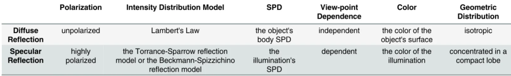
Basically, there are three characteristic differences between diffuse and specular reflections (Table 1). First, they have different degrees of polarization (the percentage of the light being polarized), which is often used in separation methods involving polarization [31,38]. Second, their intensity distributions follow different models, which are directly applied to describe and approximate these two components [24]. Third, for most inhomogeneous surfaces, the specu-lar reflection takes the illumination color because it has the relative spectral power distribution (SPD) of the illuminant. In contrast, the color of the diffuse reflection is equal to the surface color since the SPD of the diffuse reflection is altered by the object’s body SPD (resulted from interactions with colorant particles) [37,38]. This is the most common basis in reflection sepa-ration algorithms. Caused by the fundamental characteristics above, the two reflections also hold some other distinct properties, such as view-point dependence, color and geometric distri-bution, also shown inTable 1.
Dichromatic reflection model
The dichromatic reflection model [38] is a simple reflectance model to determine the linear combinations of diffuse and specular reflection components from a standard color image. The total radianceLof inhomogeneous objects is the sum of two independent terms: the radiance
Ldof the light reflected from the surface body and the radianceLsof the light reflected at the interface:
Lðl;l;v;nÞ ¼Ldðl;l;v;nÞ þLsðl;l;v;nÞ ð3Þ
whereλis the light wavelength,landvare the light source and camera viewpoint directions
Table 1. Differences of diffuse and specular reflections.
Polarization Intensity Distribution Model SPD View-point Dependence
Color Geometric
Distribution
Diffuse Reflection
unpolarized Lambert's Law the object's
body SPD
independent the color of the object's surface
isotropic
Specular Reflection
highly polarized
the Torrance-Sparrow reflection model or the Beckmann-Spizzichino
reflection model
the illumination's
SPD
dependent the color of the illumination
concentrated in a compact lobe
respectively, andnis the surface normal. Each component is decomposed into two parts:
Lðl;l;v;nÞ ¼wdðl;v;nÞcdðlÞ þwsðl;v;nÞcsðlÞ ð4Þ
The magnitude termwis a geometric scale factor which only depends on geometry shapes, while the composition termcis a relative SPD which only depends on wavelength.
Note that the diffuse magnitudewdonly depends onnandl, whereas the specular magni-tudewsalso changes with the camera viewpoint, resulting in the color intensity view angle dependent. For the sake of simplicity, we drop thelandnterms and project the scene by a digi-tal camera. Therefore, a pixelpof the image is written as:
LðpÞ ¼wdðpÞcdðpÞ þwsðpÞcsðpÞ ð5Þ
whereBandGindicate the color of the diffuse and specular reflection in the RGB channel.
Proposed Method
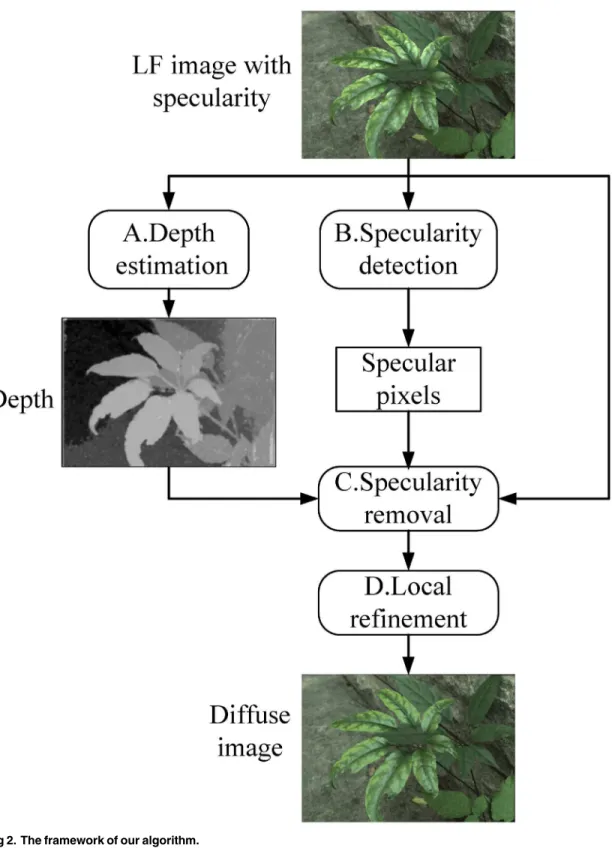
As illustrated inFig 2, our algorithm consists of four parts as depth estimation, specularity detection, specularity removal and local refinement.
Light field image depth estimation
To achieve refocusing, a robust and accurate depth map of the LF image is required. Here we utilize the dense depth estimation algorithm by integrating both defocus and correspondence cues [42]. We firstly exploit the 4D epipolar image (EPI) derived from the LF data and make shears to operate refocusing. Then we present a simple contrast-based approach to compute the responses of two cues. With both local estimated cues, we combine them with a confidence measure and compute a global depth estimation using MRFs to get the final results.
Defocus cue: Depth from defocus has been actively investigated either through using several images exposures or a complicated device to capture the data in one exposure [47]. Employing a LF camera allows us to reduce the image acquisition requirements and record multiple angu-lar information of the scene for estimating depth from defocus. Defocus measures the sharp-ness, or contrast within a patch. If a patch on a textured surface is refocused at the correct depth, it commonly provides the strongest contrast. A contrast-based measure is adopted here to find the optimalαwith the highest contrast at each pixel. By taking the sheared EPI, the average value of pixel {x,y} is calculated:
Iaðx;yÞ ¼
1
Nðu;vÞ
X
ðu0;v0ÞIaðx;y;u 0;
v0Þ ð6Þ
whereIaðx;yÞis the sheared image,N
(u,v)is the number of angular pixels (u,v). By considering
the spatial variance, the defocus cue is defined as:
Daðx;yÞ ¼ 1 jWDj
X
ðx0;y0Þ2WDjD
Iaðx0;y0Þj ð7Þ
whereWDis the window size of the current pixel andΔis the spatial Laplacian operator using the full patch. Accordingly, we obtain a defocus response for every pixel in the image at eachα.
Fig 2. The framework of our algorithm.
shearα, the matching cost for each spatial pixel is computed as the angular variance:
saðx;yÞ ¼
ffiffiffiffiffiffiffiffiffiffiffiffiffiffiffiffiffiffiffiffiffiffiffiffiffiffiffiffiffiffiffiffiffiffiffiffiffiffiffiffiffiffiffiffiffiffiffiffiffiffiffiffiffiffiffiffiffiffiffiffiffiffiffiffiffiffiffiffiffiffiffiffiffiffiffi
1
Nðu;vÞ
X
ðu0;v0ÞðIaðx;y;u
0;v0Þ Iaðx;yÞÞ2
s
ð8Þ
In an ideal case, if the matching cost for a spatial pixelpatα0is zero, it means all the angular pixels corresponding topstand for viewpoints that converge on a single point on the scene, so α0corresponds to the optimal depth. However, due to noises, occlusions and specularities, it’s rather hard to find the ideal depth, so we search for the minima of the cost. For robustness, the variance is averaged in a small windowWC:
Caðx;yÞ ¼
1
jWCj X
ðx0;y0Þ2WC
saðx
0;y0Þ ð9Þ
For each pixel, both defocus and correspondence cues are obtained at different shear values. We maximize the spatial contrast for defocus and minimize the angular variance for corre-spondence across shears to find their optimal shear valuesa
Danda
C:
a
Dðx;yÞ ¼
arg max
a Daðx;yÞ
a
Cðx;yÞ ¼
arg max
a Caðx;yÞ
ð10Þ
Since the two cues may not reach their optimal values at the sameα, their confidence are measured using Peak Ratio:
Dconfðx;yÞ ¼Da
Dðx;yÞ=DaDðx;yÞ Cconfðx;yÞ ¼Ca
Dðx;yÞ=CaDðx;yÞ
ð11Þ
whereαis the next optimalαof defocus or correspondence cue. It produces higher confi -dence when the optimalαis significantly higher or lower than others, implying the estimation is more precise.
Defocus cue operates better at occlusions, repeating patterns and noise, so it produces con-sistent but blurry depth maps. Meanwhile, correspondence cue performs more robustly at bright or dark features of the image and preserves more defined depth results at edges, but is inconsistent in noisy regions. Fortunately, confidence measures enable us to combine the reli-able region from each cue and acquire a globally optimized depthα.
Specularity detection
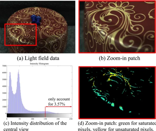
Specularity detection is essential to our algorithm. Specular pixels only account for a small per-centage for most natural images, operating removal process on all pixels wastes massive time and storage. From observation, a glossy surface often exhibits color with higher intensities than a diffuse surface of the same color. In some extreme cases, the color and intensity of illumina-tion dominate the appearance of highlights. If the light source color is uniform in every chan-nel, the highlight pixels may tend to look white. Since many state-of-the-art specularity removal methods [24,30] assume white illumination, they regard non-chromatic areas to be highlight and fail to separate specular and diffuse components in these areas.
classify specular points into“unsaturated”and“saturated”types: a saturated scene point dis-plays highlight in all (u,v) views, while an unsaturated point presents various combinations of diffuse and specular color in different views. This strategy works like this: In the central-view image, a pixelpwhose intensity is higher than a given thresholdhthresis labelled as“specular candidate”.hthrescan be adjusted within [0,255] according to the lowest intensity of specular pixels. Then, the pixels of the same candidate under all views are located by refocusing to its estimated depth and their variance are assessed. If the variance exceeds a given threshold
varthres,pis accepted as“unsaturated”. Otherwise,pis“saturated”or it reflects non-chromatic diffuse color. In implementation, we set 0.002 forvarthresand 150 forhthres.Fig 3shows an example of specularity detection.
Specularity removal
This section deals with“unsaturated”specular pixels to recover their original diffuse color. The depth map that was generated before is applied to refocus and create multiple views. For an
“unsaturated”pixel {x,y} in the central view, we remap the original LF imageI0at its depthα
(x,y) to obtain the same scene points in all (u,v) views according toEq 1. Then, conduct color analysis withinu,vof eachx,y: we use k-means clustering to classify them into two clusters in Fig 3. Specularity detection.(a) displays a LF image with the specular area (red patch) zoomed in (b). (c) shows specular candidates only take a tiny proportion of image. The detection results on the red patch are shown in (d).
HSI color space and record their centroids. We denote the cluster whose centroid has a higher intensity asdiffuse+specularset with the centroid colorM1, and the other cluster asdiffuse only
set with the centroid colorM2. Based on the dichromatic reflection model, if the magnitudewd
andwsare set to 1, the two centroids are written as:
M1¼BþG
M2¼B
ð12Þ
whereBandGrepresent the color of diffuse and specular components. With knownM1and
M2,Gcould be determined by simply subtracting the two equations.
We also offer a confidence metric to measure the accuracy for each unsaturated pixel. Assuming that higher confidence occurs at the pixel with higherM1intensity and larger
two-centroid distance, the metric is constructed as:
conf ¼expð b0
jM1j
b1
jM1 M2j
þb2
RÞ ð13Þ
whereRis the average intra-cluster distance,β0,β1,β2are constant parameters. In our
imple-mentation, bothβ0,β1are set to 0.5,β2is set to 1.
For each pixel labeled as“unsaturated”, we subtract the specular termGto restore their orig-inal diffuse color. By looking through a small window aroundx,y,u,v, we compute a weighted
Gby favouring higher confidence and smaller difference betweenI0(x,y,u,v) and its
neigh-bor’sM1. The specular component is removed by:
Idðx;y;u;vÞ ¼Iðx;y;u;vÞ hw jM1ðx
0;y0Þ M
2ðx
0;y0Þji
w¼expf g=ðConfðx0;y0Þ jIðx;y;u;vÞ M
1ðx
0;y0ÞjÞg ð14Þ
wherex0,y0are within the search window aroundx,y,u,v, andh.irepresents the expected value. We use a 15 × 15 window and 1 forγin implementation.
Local refinement
Due to the small baseline, a scene point at specular regions which is saturated in all viewpoints is common. Angularly saturated pixels exhibit the strongest intensity of the light source color and totally lose their diffuse terms. Removing specularities in the former step only takes effect on unsaturated pixels, so it may create highlight holes in the middle of the specular area where saturated pixels always occur. To remove specularities entirely, we apply a local color refine-ment to fill these holes and gain a final diffuse image. We assume that the color and texture of a point vary smoothly in its local area, which holds true for most specular images. Consequently, the color information of saturated pixels could be remedied with the color information of its neighbors.
We implement this by using K nearest neighbors. For a particular saturated pixel, we find k nearest points that are non-specular around it and assign weight to constrain the nearer neighbors contribute more to the average than more distant ones. Then, the corresponding pixels of the saturated point {x,y} in all (u,v) views are replaced by averaging its neighbors {xi,yi|i= 1,. . .k}.
Irðx;y;u;vÞ ¼ X
i¼1;...k
1
wi I0ðx
i;yi;u;vÞ; iffx;ygis saturated;
I0ðx;y;u;vÞ; others:
8 <
:
ð15Þ
Experiments & Comparisons
To validate the effectiveness of our proposed approach, we test it on multiple images with multi-color and highly textured surfaces captured by Lytro ILLUM, together with the LF images which are captured by a commercial Canon Digital camera fixed on a moving Lego Mindstorms gantry from the Stanford light field archive. For Lytro ILLUM, indoor scenarios are taken under controlled illumination condition (incandescents) and outdoor scenarios are under uncontrolled wild environment (sunlight). The camera parameters: exposure: ISO: auto, focal length: 9.5–77.8 mm (30–250 mm equivalent), lens aperture: Constantf/2.0. Considering views on the borders of the main lens do not capture light as much as the views on the center, only the central 7 × 7 views are used to construct the LF image.
We compare our work against three currently popular single-image based algorithms: Tan et al. [24], Shen et al. 30] and Yang et al. [23]. Their source code is freely available on the authors’websites [48–50]. We only make comparisons with the single-image based algorithms because the existing multiple-image based techniques require images taken under various con-ditions or have large baselines, making it impracticable to compare with them in the same set-ting. To acquire a single image input, the original LF data is refocused to the specular area. Then the diffuse output is generated under the authors’default settings. We also refocus our refined LF image at the same depth for comparison.
Qualitative analysis
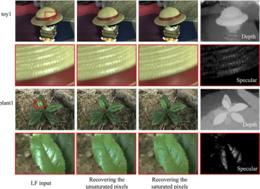
Recovering the LF diffuse image. Fig 4illustrates one indoor and one outdoor example of our proposed method. The displayed images are the 4D LF images which contains cropped
Fig 4. Two processing examples of the proposed method.The first and third rows (from left to right) display the LF input image, LF image after recovering unsaturated pixels, LF image after recovering saturated pixels, and the estimated depth of the central view. The specular area is marked by a red patch. The second and fourth rows show the zoom-in specular areas of the upper corresponding LF images, and specular components.
microlens-images, except that the depth map is from the central pinhole image. By zooming in the specular area on the hat and the leaf, we easily observe that unsaturated and saturated pixels are correctly restored to their original diffuse color in two steps. The close-up patch of specular component is also provided. Note that the color of specular components have been enhanced for easier visibility throughout this paper.
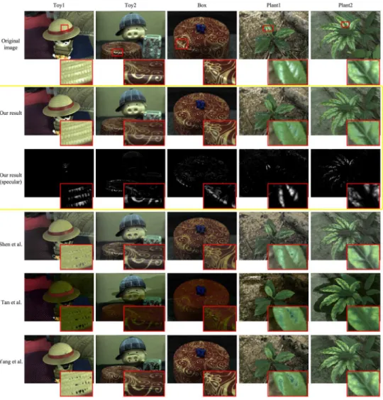
Diffuse results for Lytro ILLUM images. InFig 5, the indoor and outdoor objects have glossy surfaces which are marked by red rectangles. Our approach correctly weakens the specu-lar intensity, successfully recovers diffuse color, and well preserves the consistency of other regions, while Shen, Tan and Yang can cause obvious mistakes, particularly at white and tex-tured areas. In detail, Shen’s method creates black holes on the non-chromatic area (the eyes in Toy1 and nose in Toy2) and the highlight in Plant1 is not removed completely yet. Besides, the color of diffuse areas slightly differs to the original image (the hat in Toy1, the face in Toy2). Anyway, it produces good results on five images. About the color information, Tan’s results are significantly darker than the original images and bring easy-to-see errors, e.g. losing color
Fig 5. Diffuse results for Lytro ILLUM images.The first row shows the refocused original images and their corresponding zoom-in specular areas. The second and third rows are diffuse and specular images of our proposed method. The other three rows are the diffuse images of Shen et.al. [30], Tan et.al. [24] and Yang et. al. [23].
consistency, losing texture information and creating inexistent edges. Yang produces compara-tive results in Plant2 and Box, but gives rise to black holes in Toy1 and Toy2 and inconsistent color in Plant1. Non-specular areas have been ruined to different degrees in these methods, which largely reduce image quality. The results show our algorithm outperforms them.
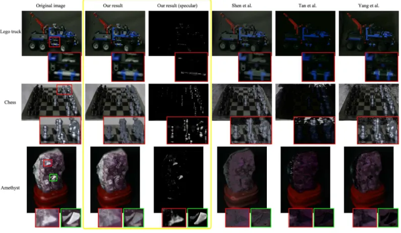
Diffuse results for Stanford light field archive images. Fig 6illustrates three challenging images from the Stanford light field archive. The first image is a Lego Technic truck which has very complex geometry. Our proposed method properly reduces the highlight on the wheels without damaging its geometry and brightness. The second image is a chess board with pieces, which have specular reflections of various intensities. Compared to our diffuse result, Tan loses almost all the information of the image while Shen and Yang destroy the color constancy of background. The last is a chunk of amethyst with interesting specularities and some translu-cency. After the processing steps for unsaturated and saturated pixels, strong highlights in red and green rectangles are removed acceptably. However, the rest methods fail at it.
Quantitative analysis
Subjective evaluation metrics. To evaluate our approach in a quantized way, we invite 50 volunteers from different gender and age to score the specular removal results of all methods. Given an image with specular items, human’s brain can automatically fix the specular parts and illustrate the diffuse version of this image. Since it’s rather individual dependent, for each image, we omit the highest/lowest score and average scores to decrease subjective bias. For every image, the volunteers are required to rate two indexes: SA and IQ. SA is for specularity
Fig 6. Experiments of the Stanford light field archive.
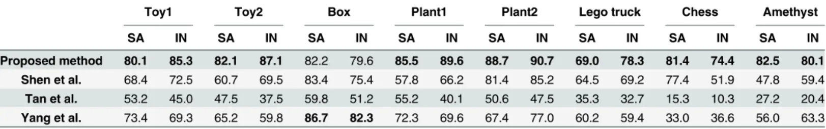
accuracy, which is graded based on the accuracy of specular components separated by each method compared with the one he has in mind. IN is for image naturalness because preserving naturalness is essential for highlight removal methods to achieve pleasing perceptual quality. Both the two scores are ranging from 0~100, where 0~20 means very poor, 20~40 means poor, 40~60 means fair, 60~80 means good and 80–100 means very good. The greater value of the score, the better quality of the image. The average scores are shown inTable 2, clearly our algo-rithm is superior to the other three methods in most specular images.
Objective evaluation metrics. The volunteers are also asked to mark the areas where high-lights occur. We average the manually marked regions and regard them as the highlight area ground truth to provide an objective evaluation. Note that this manually marked regions doesn’t contain the highlight intensity information, so we change the specular component image of each scene to a binary image under the control of the same threshold. Then the basic measures used in evaluating classification results: precision, recall and F-measure (harmonic mean of precision and recall compared to ground truth) are calculated to test the accuracy of highlight detection, as shown in Tables3,4and5. From our observation, people tend to draw Table 2. The scores of the specular removal results.
Toy1 Toy2 Box Plant1 Plant2 Lego truck Chess Amethyst
SA IN SA IN SA IN SA IN SA IN SA IN SA IN SA IN
Proposed method 80.1 85.3 82.1 87.1 82.2 79.6 85.5 89.6 88.7 90.7 69.0 78.3 81.4 74.4 82.5 80.1 Shen et al. 68.4 72.5 60.7 69.5 83.4 75.4 57.8 66.2 81.4 85.2 64.5 69.2 77.4 51.9 47.8 59.4
Tan et al. 53.2 45.0 47.5 37.5 59.8 51.2 55.2 40.1 50.6 47.5 35.3 32.7 15.3 10.3 27.2 20.4
Yang et al. 73.4 69.3 65.2 59.8 86.7 82.3 72.3 69.6 67.4 77.0 60.2 59.4 33.0 36.6 56.0 63.3
doi:10.1371/journal.pone.0156173.t002
Table 3. The precision of the specular removal results.
Toy1 Toy2 Box Plant1 Plant2 Lego truck Chess Amethyst
Proposed method 0.9634 0.8570 0.8121 0.8681 0.7862 0.3152 0.7137 0.8311
Shen et al. 0.0548 0.7198 0.9952 0.0381 0.8293 0.1257 0.0230 0.0664
Tan et al. 0.0402 0.0823 0.4067 0.0073 0.0425 0.0528 0.0496 0.0759
Yang et al. 0.0656 0.2488 0.8832 0.0303 0.0691 0.0643 0.0263 0.0699
doi:10.1371/journal.pone.0156173.t003
Table 4. The recall of the specular removal results.
Toy1 Toy2 Box Plant1 Plant2 Lego truck Chess Amethyst
Proposed method 0.5313 0.2024 0.3121 0.3379 0.3274 0.3042 0.6522 0.5155
Shen et al. 0.1573 0.2625 0.2046 0.0070 0.1173 0.4857 0.3780 0.4809
Tan et al. 0.9676 0.7911 0.3734 0.1103 0.5158 0.7771 0.9873 0.6572
Yang et al. 0.2940 0.4354 0.2643 0.0752 0.1914 0.5139 0.2364 0.6336
doi:10.1371/journal.pone.0156173.t004
Table 5. The F-measure of the specular removal results.
Toy1 Toy2 Box Plant1 Plant2 Lego truck Chess Amethyst
Proposed method 0.6849 0.3275 0.4509 0.4865 0.4623 0.3096 0.6816 0.6363
Shen et al. 0.0813 0.3847 0.3394 0.0118 0.2055 0.1997 0.0434 0.1167
Tan et al. 0.0772 0.1491 0.3893 0.0137 0.0785 0.0989 0.0945 0.1361
Yang et al. 0.1073 0.3167 0.4068 0.0432 0.1015 0.1143 0.0473 0.1259
lines around the relatively stronger and larger highlight areas, and overlook weak and small ones. Our algorithm has a higher precision than other methods among most images while the recall of ours is actually common. The F-measure, which take the performance of both preci-sion and recall into consideration, demonstrates the effectiveness of our method. The precipreci-sion of other techniques is much lower because non-chromatic (white or gray) areas which they regard as highlights are possibly not included in the manually marked highlights. In addition, Tan achieves a considerably high recall, but it suffers from a poor precision, because it includes most true highlight pixels at the expense of even more detected false highlights.
Conclusions
We have presented a novel and accurate specular reflection removal methodology based on light field imaging, which extensively exploits the spatial and angular information of the 4D LF together with the characteristics of diffuse and specular reflections. In our methodology, the diffuse image is first recovered by removing the specular effects on“unsaturated”pixels, and then refined locally on“saturated”pixels. The classification and recovering steps on two types of specular pixels makes our approach applicable to various surfaces with more complex and stronger highlights. We have experimented on multiple real world LF images from our Lytro ILLUM and the Stanford light field archive with both qualitative and quantitative analysis. The results demonstrate that our algorithm achieve excellent performance, especially in non-chro-matic and textured areas, while properly preserving color constancy on non-specular areas. Still, our method does not work well at mirrors or extremely specular surfaces. Achieving higher accuracy of specularity detection and improving robustness of a larger area of highlight are left as future works.
Acknowledgments
This work is partially supported by the NSFC fund (61471213), Shenzhen Fundamental Research fund (JCYJ20140509172959961), Natural Science Foundation of Guangdong Prov-ince (2015A030310173), National High-tech R&D Program of China (863 Program,
2015AA015901) and the Science and Technology Planning Project of Sichuan Province under Grant 2014SZ0207.
Author Contributions
Conceived and designed the experiments: CXX XZW. Performed the experiments: CXX XZW. Analyzed the data: HQW CXX XZW YBZ BP. Contributed reagents/materials/analysis tools: HQW CXX XZW YBZ BP. Wrote the paper: HQW CXX XZW YBZ BP.
References
1. Artusi A, Banterle F, Chetverikov D. A survey of specularity removal methods. Computer Graphics Forum. 2011 Aug 2; 30(8): 2208–30.
2. Tan P, Lin S, Quan L, Shum HY. Highlight removal by illumination-constrained inpainting. Proceedings of IEEE International Conference on Computer Vision (ICCV); 2003 Oct 13–16; IEEE Computer Soci-ety; 2003.
3. Lam CP, Yang AY, Elhamifar E, Sastry SS. Multiscale TILT Feature Detection with Application to Geo-metric Image Segmentation. Proceedings of IEEE International Conference on Computer Vision Work-shops (ICCVW); IEEE Computer Society; 2013.
4. Heo YS, Lee KM, Lee SU. Robust stereo matching using adaptive normalized cross-correlation. IEEE Trans. Pattern. Anal. Mach. Intel. 2011 Apr; 33(4): 807–22.
6. Shen L, Bai L, Ji Z. FPCODE: An efficient approach for multi-modal biometrics. International Journal of Pattern Recognition and Artificial Intelligence. 2011; 25(2): 273–86.
7. Liu F, Zhang D, Shen L. Study on novel curvature features for 3D fingerprint recognition. Neurocomput-ing. 2015; 168(1): 599–608.
8. Zhu Z, Jia S, He S, Sun Y, Ji Z, Shen L. Three-dimensional gabor feature extraction for hyperspectral imagery classification using a memetic framework. Information Sciences. 2015; 298(1): 274–87.
9. Jian M, Lam KM, Dong J, Shen L. Visual-patch-attention-aware saliency detection. IEEE Transactions on Cybernetics. 2015; 45(8): 1575–86. doi:10.1109/TCYB.2014.2356200PMID:25291809
10. Kong H, Lai Z, Wang X, Liu F. Breast Cancer Discriminant Feature Analysis for Diagnosis via Jointly Sparse Learning. Neurocomputing. 2016 Feb; 177: 198–205.
11. Li K, Yang J, Jiang J. Nonrigid Structure From Motion via Sparse Representation. IEEE Transactions on Cybernetics.2015 Aug; 45(8): 1401–13. doi:10.1109/TCYB.2014.2351831PMID:26186752
12. Zhu Y, Li K, Jiang J. Video super-resolution based on automatic key-frame selection and feature-guided variational optical flow. Signal Processing: Image Communication.2014 Sep; 29(8): 875–86.
13. Yang Y, Wang X, Liu Q, Xu M, Yu L. A bundled-optimization model of multiview dense depth map syn-thesis for dynamic scene reconstruction. Information Sciences. 2015 Nov; 320: 306–19.
14. Yang Y, Wang X, Guan T, Shen J, Yu L. A multi-dimensional image quality prediction model for user-generated images in social networks. Information Sciences. 2014 Oct 10; 281: 601–10.
15. Zhang J, McMillan L, Yu J. Robust tracking and stereo matching under variable illumination. Proceed-ings of IEEE Conference on Computer Vision and Pattern Recognition; IEEE Computer Society; 2006.
16. Lin S, Li Y, Kang SB, Tong X, Shum HY. Diffuse-specular separation and depth recovery from image sequences. Computer Vision—ECCV 2002. 2002; 210–24.
17. Nayar SK, Krishnan G, Grossberg MD, Raskar R. Fast separation of direct and global components of a scene using high frequency illumination. ACM Transactions on Graphics (TOG). 2006; 25(3): 935–44.
18. Lai Z, Xu Y, Chen Q, Yang J, Zhang D. Multilinear sparse principal component analysis. IEEE Transac-tions on Neural Networks and Learning Systems. 2014; 25(10): 1942–50. doi:10.1109/TNNLS.2013. 2297381PMID:25291746
19. Lai Z, Wong W, Xu Y, Yang J, Tang J, Zhang D. Approximate orthogonal sparse embedding for dimensionality reduction. IEEE Transactions on Neural Networks and Learning Systems.2015; 27(4): 723–35. doi:10.1109/TNNLS.2015.2422994PMID:25955995
20. Wong W, Lai Z, Xu Y, Wen J. Joint tensor feature analysis for visual object recognition. IEEE Transac-tions on Cybernetics. 2015; 45(11): 2425–36. doi:10.1109/TCYB.2014.2374452PMID:26470058
21. Zhu Z, Jia S, Ji Z. Towards a memetic feature selection paradigm. IEEE Computational Intelligence Magazine. 2010; 5(2): 41–53.
22. Lai Z, Wong W, Xu Y. Sparse alignment for robust tensor learning. IEEE Transactions on Neural Net-works and Learning Systems. 2014; 25(10): 1779–92. doi:10.1109/TNNLS.2013.2295717PMID: 25291733
23. Yang Q, Tang J, Ahuja N. Efficient and Robust Specular Highlight Removal. IEEE Trans. Pattern. Anal. Mach. Intel. 2015 Jun; 37(6): 1304–11.
24. Tan RT, Ikeuchi K. Separating reflection components of textured surfaces using a single image. IEEE Trans. Pattern. Anal. Mach. Intel. 2005 Feb; 27(2): 178–93.
25. Tao MW, Wang TC, Malik J, Ramamoorthi R. Depth estimation for glossy surfaces with light-field cam-eras. Computer Vision—ECCV 2014 workshops. 2014; 533–47.
26. Raskar R, Tumblin J. Computational Photography: Mastering New Techniques for Lenses, Lighting, and Sensors. Natick: AK Peters; 2009.
27. Levoy M, Hanrahan P. Light field rendering. Proceedings of the 23rd annual conference on Computer graphics and interactive techniques. ACM; 1996.
28. Gortler SJ, Grzeszczuk R, Szeliski R, Cohen MF. The lumigraph. Proceedings of the 23rd annual con-ference on Computer graphics and interactive techniques. ACM; 1996.
29. Adams A. The (New) Stanford Light Field Archive. 2008. Available:http://lightfield.stanford.edu/lfs.html.
30. Shen HL, Zhang HG, Shao SJ, Xin JH. Chromaticity-based separation of reflection components in a single image. Pattern Recognition. 2008; 41(8): 2461–9.
31. Nayar SK, Fang XS, Boult T. Separation of reflection components using color and polarization. Interna-tional Journal of Computer Vision. 1997; 21(3): 163–86.
33. Lin S, Shum HY. Separation of diffuse and specular reflection in color images. Proceedings of IEEE Conference on Computer Vision and Pattern Recognition; IEEE Computer Society; 2001.
34. Lee SW, Bajcsy R. Detection of specularity using color and multiple views. Computer Vision—ECCV 1992. 1992; 99–114.
35. Criminisi A, Kang SB, Swaminathan R, Szeliski R, Anandan P. Extracting layers and analyzing their specular properties using epipolar-plane-image analysis. Computer vision and image understanding. 2005; 97(1): 51–85.
36. Bajcsy R, Lee SW, Leonardis A. Detection of diffuse and specular interface reflections and inter-reflec-tions by color image segmentation. International Journal of Computer Vision. 1996; 17(3): 241–72.
37. Klinker GJ, Shafer SA, Kanade T. The measurement of highlights in color images. International Journal of Computer Vision. 1988; 2(1): 7–32.
38. Shafer SA. Using color to separate reflection components. Color Research & Application. 1985; 10(4): 210–18.
39. Shen HL, Cai QY. Simple and efficient method for specularity removal in an image. Applied optics. 2009; 48(14): 2711–19. PMID:19424394
40. Nguyen T, Vo QN, Kim SH, Yang HJ, Lee GS. A novel and effective method for specular detection and removal by tensor voting. Proceedings of IEEE Conference on Image Processing; IEEE Computer Society; 2014.
41. Ng R, Levoy M, Bredif M, Duval G, Horowitz M, Hanrahan P. Light field photography with a hand-held plenoptic camera. Computer Science Technical Report CSTR. 2005; 2(11).
42. Tao MW, Hadap S, Malik J, Ramamoorthi R. Depth from combining defocus and correspondence using light-field cameras. Proceedings of IEEE International Conference on Computer Vision (ICCV); IEEE Computer Society; 2013.
43. Jeon HG, Park J, Choe G, Park J, Bok Y, Tai YW et al. Accurate Depth Map Estimation from a Lenslet Light Field Camera. Proceedings of IEEE Conference on Computer Vision and Pattern Recognition; IEEE Computer Society; 2015.
44. Li N, Ye J, Ji Y, Ling H, Yu J. Saliency detection on light field. Proceedings of IEEE Conference on Com-puter Vision and Pattern Recognition; IEEE ComCom-puter Society; 2014.
45. Cho D, Kim S, Tai YW. Consistent Matting for Light Field Images. Computer Vision–ECCV 2014. 2014; 90–104.
46. Bishop TE, Zanetti S, Favaro P. Light field superresolution. Proceedings of IEEE International Confer-ence on Computational Photography (ICCP); IEEE Computer Society; 2009. p. 1–9.
47. Watanabe M, Nayar SK. Rational filters for passive depth from defocus. International Journal of Com-puter Vision. 1998; 27(3): 203–25.
48. Tan's sourcecode. Available:http://php-robbytan.rhcloud.com/textureSeparation/results.html.
49. Shen's sourcecode. Available:http://www.ivlab.org/publications.html.