Application of Wavelet LPC Excitation Model for Speech Compression

Application of Wavelet LPC Excitation Model for Speech

Compression

1,2_{Armein Z.R. Langi}

1

Research Center on Information and Communication Technology 2

Information Technology RG, School of Electrical Engineering and Informatics Institut Teknologi Bandung, Jalan Ganeca 10, Bandung, 40116, Indonesia

Abstract. This paper presents an application of linear predictive coding (LPC) excitation wavelet models for low bit- rate, high-quality speech compression. The compression scheme exploits the model properties, especially magnitude dependent sensitivity, scale dependent sensitivity, and limited frame length. We use the wavelet model in an open-loop dither based codebook scheme. With this approach, the compression yields a signal-to-noise ratio of at least 11 dB at rates of 5 kbit/s and.

Keywords: LPC; LPC excitation; modelling; speech compression; speech processing; wavelets.

1

Introduction

Speech signal compression is a necessity in speech communication either because of an operational requirement based on a design constraint, or because of the desire to utilize existing resources efficiently [1]. In a pulse code modulation (PCM) form, real-time telephone-quality speech requires a rate of 64 kbit/s, which is too high for high frequency (HF) radio or practical network channels. At this rate, speech as short as one minute would also occupy large storage space (480 kbytes).

LPC excitation models play a critical role to obtain high speech quality at low bit- rates. At the present time, advanced techniques such as line-spectrum pair (LSP) can successfully code the filter parameters at as low as 0.75 - 1 kbit/s, with average spectral distortion less than 1 dB [3-4]. However, that is not the case for the LPC excitation. As it is, it would require a 64 kbit/s rate. There are different techniques to code the excitation based on different models, with a trade off between the resulting quality and the bit rate. One very efficient model used in the LPC-10e consists of a pitch impulse generator, a random impulse generator, a gain controller, and a voiced/unvoiced (V/UV) switch, resulting in a machine-quality speech. The CELP uses a stochastic codebook and an adaptive codebook, resulting in good speech-quality [5]. Another model uses scalar quantization or centre-clipping in conjunction with a pitch filter, as in adaptive differential PCM (ADPCM). This technique results in high speech quality at bit rates of 16 to 32 kbit/s.

The linear combination of wavelets is an attractive model of LPC excitation for speech compression [6-7]. Such a wavelet model of LPC excitation has been shown to have asymmetrical and nonuniform properties that are attractive for speech compression, namely magnitude dependent sensitivity, scale dependent sensitivity, and limited frame length. This paper proposes new speech compression schemes using that model. The schemes exploit those coefficients’ asymmetrical properties. Our specific contributions are (1) an ideal scheme through the use of close-loop codebook searching and perceptually weighted measure, as well as (2) a practical scheme through whitening the effect of the quantization noise. Our experiment shows that even in a simple straight-forward implementation, the model indicates promising capability by having SNR 11.03 and 15.33 dB at 5 and 5.5 kbit/s, respectively.

2

The Wavelet Model of LPC Excitation

In this section, we review the wavelet model of LPC excitation as well as its properties.

2.1

LPC excitation

We can use a segment of speech signal s[n] to obtain LPC excitation t[n]. Let an LPC filter H(z) be [8].

 

10 1

0 1

) (



  

    

   





i

i iz a z

A z

In the z-domain, the speech segment S

 

z , LPC excitation T

 

z , and the LPC filter H

 

z are related by

 

z H

   

zT z

S  (2)

A similar relationship can be defined in vector notations. Let the segment of speech be s, which is a vector whose elements are s[0], s[1], ..., s[N–1]. A linear prediction procedure [8] can obtain ai in Eq. (1) from such s. Let hi be

the impulse responses of H(z). We can the represent H(z) in an N×N lower-triangular matrix H [9]:

             

1 2 0

0 1 0 0 0 0 h h h h h h H N N        (3)

We can now represent the LPC excitation with a vector t, whose elements are t[0], t[1], ..., t[N–1], in which s = Ht.

However H(z) is an all-pole filter, containing memory. Hence one s[n] is affected by all t[m], with m ≤ n. Thus, there is an additive contribution of all t[m] from the previous segments to the current s, denoted as a vector u. Taking this into consideration, Eq. (2) becomes

t = H−1 (s−u) (4)

In paractive, this t should be modelled and compressed without any consideration of u, since a speech production filter in Eq. (2) automatically generates u.

2.2

The Wavelet Model

The LPC excitation can be seen as a linear-combination of wavelets. Consider a set of signals which are members of RN, grouped into two subsets



_j,k

 

n



and

 



_J,k n



. Here, J is any integer between 1 and log2N. (In this work, we set J to

(log2N)–1). Index j is called scale, ranging from 1, 2, ..., to J, while k is 0, 1, ...,

to (2–jN)–1. Signals in both subsets are called wavelet and scaling signals, respectively. Then, there are real numbers cj,k and dJ,k, called waveletcoefficients

and scalingcoefficients [10] defined as

 

 



   1 0 , , N n k j k

j tn n

c  and



   

   1 0 , , N n k J k

J tn n

With these coefficients, we can express t as a linear combination of wavelets as follows.

 

_{ }

 

_



 

 





 



 2 1

0 , , 1

1 2

0 , ,

N

k

k J k J J

j N

k

k j k j

j j

n d

n c

n

t   (6)

Eqs. (5) and (6) also represent forward and inverse DWT of t, respectively.

2.3

Properties

Other work has shown that the wavelet coefficients have attractive properties:

1. The high-magnitude coefficients are more important than the low-magnitude ones, thus we can coarsely quantize the low-low-magnitude coefficients. Furthermore, there are more low-magnitude coefficients than the high-magnitude ones, making the bit-rate even lower.

2. The coefficients in a certain scale are more important than the coefficients in the other scales, thus we can coarsely quantize the coefficients in the other scales. Furthermore, the number of important coefficients is less than that of the other coefficients, making it attractive for lossy compression.

3. What is the best length of frame (N) for t to use? The frame length must be limited to reduce coding delay and system complexity. In discrete Fourier transform (DFT), the answer to this important question determines the uniform sampling resolution in frequency domain. The longer the frame is, the finer the frequency resolution. However, this is not the case in our model. The optimal N is among 32, 64, and 128 points.

3

Proposed Compression Schemes

The model can then be used to build compression schemes. The key is to compress the excitation, which is a collection of wavelet coefficients.

3.1

Compressing the Excitation

WAVELET TRANSFORM LPC Excitation Wavelet Coefficients COEFFICIENT QUANTIZATION/ ENCODING Compressed Excitation

 

 

 

          _{ }  1 , , 2 1 , 2 ; 1 2 , , 1 , 0 ; ) ( ), ( , N N N i n N i n n

v _{J J}

i k i j J i J i     (7) where

 

k i i N

N i i

j int log_{2 }; () 2j(i)

             (8)

Notice that the function int(•) returns the maximum integer value that does not

exceed the argument. Consequently, we can define c which satisfies both Eq. (4) and Eq. (6), by assigning ordered values of {cj,k, dJ,k} as the elements of

c

_i.

Clearly, the order must follow that of the scaling and wavelet functions in the vi

above. Thus, we have Eq. (6) to be

 

_



 

  1 0 N i i iv n c n

t (9)

Here, the DWT becomes a mapping :



tc



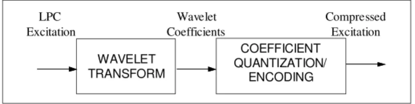
, and its inverse 1 is Eq. (9).

To compress t, we usually must approximate the set of coefficients c_i with cˆ_i which uses fewer bits, shown in Figure 1. First the encoder converts the LPC excitation into wavelet coefficients c_i. It then quantizes c_i into cˆ_i and compress it. With this approach, we can have an efficient representation of the excitation.

Figure 1 Wavelet encoder.

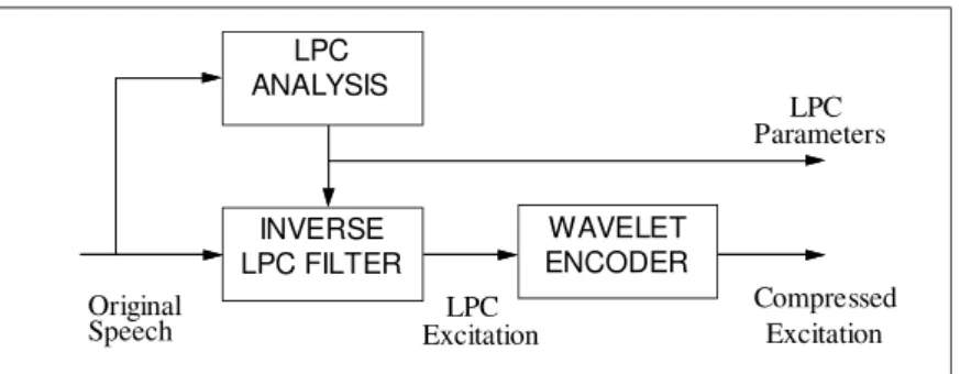
WAVELET ENCODER INVERSE

LPC FILTER LPC ANALYSIS

Original Speech

LPC Parameters

LPC Excitation

Compressed Excitation

Figure 2 Conceptual speech compressor (analyzer).

In this approach, a speech decompressor would have a scheme as in Figure3. It contains a wavelet decoder. A wavelet decoder first decodes the compressed excitation into the wavelet coefficients. It then inverse transforms the coefficients, resulting in LPC excitation. An LPC filter uses transmitted LPC coefficients to produce reconstructed speech from LPC excitation.

INVERSE WAVELET TRANSFORM

LPC Excitation Wavelet

Coefficients

LPC FILTER

Reconstructed Speech

COEFFICIENT DECODING Excitation

Compressed

LPC Coefficients WAVELET DECODER

Figure 3 Speech decompressor (synthesizer).

However, this approximation introduces error (distortion) that should be minimized. Notice that in the wavelet decoder, the coefficient set results in excitation tˆ

 

n , which would produce sˆ

 

n instead of s

 

n in Eq. (2). Since the distortion occurs at the excitation, the LPC filter will enhanced the error according to speech magnitudes. In other words, the distortion correlates with the speech. This results in disturbing and unpleasant speech distortion.

 





_{ }





   



 

 

   

  

 



 1

0

2 1

0

, ˆ

ˆ ˆ

,

N

i N

j j

i s j s j w

s s W s s

d (10)

We can reformulate the error measure in Eq. (13) in terms of c, as also derived in [11].

 

s s W



s s



WH

 

t t WH



c c



d ,ˆ  ˆ  ˆ  1 ˆ (11)

If Q be an N×N matrix whose i-th column is vi, we immediately have Eq. (9) to

be

t = Qc (12)

We can now simplify Eq. (10) by first defining T[c] as a mapping of c as

T[c] = WHQc (13)

and then rewrite Eq. (10) as

 

s s T



c c



d ,ˆ  ˆ (14)

Since T[] is linear, the upper-bound of the error is

 

s s T c c

d ,ˆ  ˆ (15)

(The norm definition of Eq (10) must be one that is compatible with Euclidean norm of vectors). Clearly we must minimize

c



c

ˆ

so that we minimize the

upper-bound. However, this rather simple minimization is not sufficient, because T changes with s. There are cases where minimizing ccˆ does not minimize Eq. (14), because

c



c

ˆ

is not generally an eigenvector of T. Thus, we must focus on minimizing Eq. (14) instead of minimizing ccˆ alone.

Although we can use the scheme in Figure 6, the distortion correlates to speech. In practice we can improve the quality using two options of quantizing c. First option is a close-loop searching through a set of codebooks. Second option is an open-loop scheme through noise whitening.

3.2

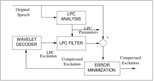
An Ideal Closed-Loop Scheme

scheme uses a set of codebooks to store a limited set of cˆ in the place of coefficient decoding (see Figure 7). However, the analyzer becomes a scheme in Figure 4. Here, the compressed excitation is search from the codebooks through the close-loop trials. This closed-loop search uses minimum d

 

s,sˆ as its criterion, ensuring its closeness.

However such quality comes with the expense of very high computing requirements. Searching the codebook through close-loop trials involves inverse transform, LPC filtering as well distance measures for each trial. As a result, such an ideal solution is not practical.

ERROR MINIMIZATION LPC FILTER

LPC ANALYSIS

Original Speech

LPC Parameters

LPC

Excitation _Compressed

Excitation

WAVELET DECODER

Compressed Excitation

+

–

Figure 4 A closed-loop analyzer.

3.3

A Practical Open-Loop Scheme

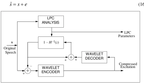
Alternatively we should look at an open-loop approach but still maintains uncorrelated distortion. The second scheme rearranges the analyzer in Figure 2 to obtain white noise effect (instead of correlated one) of the quantization noise on the resulting speech. If the quantization noise has correlation with the speech, the noise is more perceivable [5]. Although the quantization itself can result in coefficient error that is uncorrelated with the coefficients, the speech error still correlates with speech signal, because the filter H(z) shapes the error spectrum.

e

s

s

ˆ





(16)

WAVELET ENCODER 1–H–1( )z

LPC ANALYSIS

s

LPC Parameters

Compressed Excitation

+ –

WAVELET DECODER

+ +

Original Speech

Figure 5 Speech compressor, with white-noise effect on the reconstructed speech.

4

Experimental Results

There are many schemes that can be used to exploit the properties described earlier. In principle, every scheme that uses LPC excitation can adopt the model. Here, we simply use the scheme as in Figure 2 and Figure 3 for our experiment, with slight modifications in the wavelet encoder/decoder. We incorporated LSP coding for the LPC coefficients at a rate of 1 kbit/s.

The wavelet encoder consists of a normalizer, a wavelet transformer, and a limited size codebook, as shown in Figure 6. The normalizer computes the gain factor of the LPC excitation and extracts that from the LPC excitation, so that the variance of the input of the wavelet transformer is one.

WAVELET

TRANSFORM NORMALIZER

VARIANCE

ESTIMATION

LPC Excitation

Code Book Indices Gain

CODEBOOK

ENCODING

Figure 6 Wavelet encoder.

To reconstruct the speech, we use the inverse process depicted in Figure 7. The process passes the parameters to the codebooks, inverses transforms the resulting codeword, scales the resulting excitation signal according to the gain factor, and applies the resulting signal to an LPC filter.

INVERSE WAVELET TRANSFORM CODEBOOKS

LPC Excitation Code Book

Indices

LPC FILTER

Gain Reconstructed

Speech

Figure 7 Speech decompressor.

We design a codebook for every scale using frequency-sensitive competitive learning neural network [12]. Thus, for the frame length of 64, there should be 6 codebooks. However, based on the properties discussed above, we decided to include scale 1, 2, 3, and 4 only, and omit scale 5 and the lowpass section. Thus, we have designed four codebooks with two different sizes, 128 and 256, and trained them using the coefficients obtained from training sentences.

By combining the codebooks, we can have different sets of codebooks with different numbers of bits required between 28 to 32 bits per 64 samples. For two sets with 28 and 32 bits per 64 samples, we need 3.5 and 4.0 kbit/s, respectively. Assuming that the gain factor requires 4 bits per 64 samples, i.e., 0.5 kbit/s, and LPC coefficients require 1 kbit/s, the two sets result in 5 and 5.5 kbit/s, respectively.

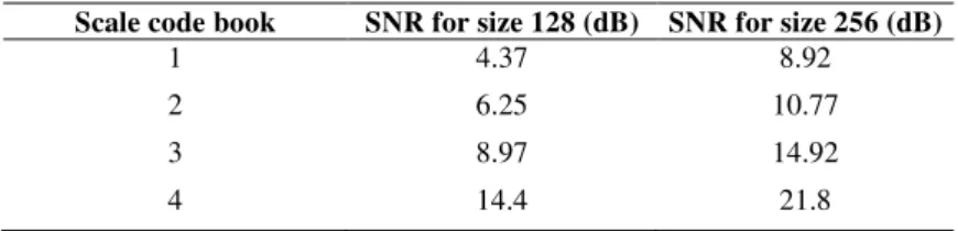
sentences [5] for training as well as test. We then perform speech compression and decompression in two different sets of codebooks. The codebooks have a size of 128 and 256, respectively. The neural network was able to distribute the codewords among the training set. For the given codebook sizes, the SNR of the coefficients were low, as depicted in Table 1. Those are SNR for wavelet coefficients related to excitations.

Table 1 SNR of wavelet coefficients for each scale codebook.

Scale code book SNR for size 128 (dB) SNR for size 256 (dB)

1 4.37 8.92

2 6.25 10.77

3 8.97 14.92

4 14.4 21.8

However, when the excitations are applied to LPC filter, the speech SNR improves significantly. Thank to the power of the model, the speech SNR measurement with 128 and 256 sizes of codebooks results in 11.03 and 15.33 dB, respectively, which are quite high for their bit rates. Although these results are preliminary due to the limited number of test sentences, they show the promising potential of the wavelet model.

Table 2 SNR of the synthesized speech.

Code book size Bit rate (kbit/s) SNR (dB)

128 5 11.03 256 5.5 15.33

5

Conclusions

Acknowledgements

This work was supported in part by the Natural Sciences and Engineering Research Council (NSERC) of Canada, and Riset Unggulan Terpadu (RUT). The author acknowledges Dr. Ken Ferens, University of Manitoba, Canada, for his contribution in neural network based codebook design, used in this result.

References

[1] Markovic, M.Z, Speech Compression - Recent Advances and Standardization, 5th International Conference on Telecommunications in Modern Satellite, Cable and Broadcasting Service, 2001, TELSIKS 2001,

1, Page(s): 235 – 244, 19-21 Sept. 2001.

[2] Campbell, Jr. J. P., Tremain, T. E. & Welch, V. C., The proposed Federal Standard 1016 4800 bps voice coder: CELP, Speech Technology, pp. 58-64, Apr./May 1990.

[3] Paliwal, K.K. & Atal, B.S., Efficient Vector Quantization of LPC Parameters at 24 bits/ frame, IEEE Trans. Speech Audio Proc., IEEE 1063-6676/93, vol. 1, no. 1, pp. 3-14, Jan 1993.

[4] Soong, F. K. & Juang, B-H, Optimal Quantization of LSP Parameters, IEEE Trans. Speech Audio Proc., IEEE 1063-6676/93, 1(1), pp. 15-24, Jan 1993.

[5] Langi, A., Code-Excited Linear Predictive Coding for High-Quality And Low Bit-Rate Speech, M.Sc. Thesis, University of Manitoba, Winnipeg, MB, Canada, 138 pp., 1992.

[6] Najih, A.M.M.A., Ramli, A.R., Ibrahim, A., Syed, A.R., Comparing speech compression using wavelets with other speech compression schemes, Proceedings, Student Conference on Research and Development, 2003, SCORED 2003, P:55 – 58, 25-26 Aug. 2003.

[7] Najih, A.M.M.A., bin Ramli, A.R., Prakash, V., Syed, A.R., Speech compression using discreet wavelet transform, NCTT 2003 Proceedings. 4th National Conference on Telecommunication Technology, pp1 – 4, 14-15 Jan. 2003.

[8] Parsons, T. W., Voice and Speech Processing. New York: McGraw-Hill, 402 pp., 1986.

[9] Atal, B.S., A model of LPC excitation in terms of eigenvectors of the autocorrelation matrix of the impulse response of the LPC filter, in Proc. IEEE ICASSP, CH2673-2/89, pp. 45-48, 1989.

[11] Ofer, E. D., Malah, Dembo, A., A Unified Framework for LPC Excitation Representation in Residual Speech Coders, in Proc. IEEE ICASSP, CH2673-2/89, pp. 41-44, 1990.

[12] Ferens, K. & Kinsner, W., Energy and Frequency Adaptive Wavelet Subband Coding for Wideband Audio Compression, Proc. 9th Int. Conf. on Math. and Comp. Modelling, 1993.