A coupled two-dimensional hydrodynamic and terrestrial input model to simulate CO<sub>2</sub> diffusive emissions from lake systems

(1)

GMDD

6, 3509–3556, 2013

Modeling CO2

diffusive emissions from lake systems

H. Wu et al.

Title Page

Abstract Introduction

Conclusions References

Tables Figures

◭ ◮

Back Close

Full Screen / Esc

Printer-friendly Version

Interactive Discussion

Discussion

P

a

per

|

Dis

cussion

P

a

per

|

Discussion

P

a

per

|

Discussio

n

P

a

per

|

Geosci. Model Dev. Discuss., 6, 3509–3556, 2013 www.geosci-model-dev-discuss.net/6/3509/2013/ doi:10.5194/gmdd-6-3509-2013

Geoscientiic Geoscientiic

Geoscientiic

Open Access

Geoscientiic Model Development Discussions

This discussion paper is/has been under review for the journal Geoscientific Model Development (GMD). Please refer to the corresponding final paper in GMD if available.

A coupled two-dimensional hydrodynamic

and terrestrial input model to simulate

CO

₂

di

_ff

usive emissions from lake

systems

H. Wu1,2, C. Peng2,3, M. Lucotte2,4, N. Soumis2,4, Y. G ´elinas5, ´E. Duchemin2,4, J.-B. Plouhinec2,4, A. Ouellet5, and Z. Guo1

1

Key Laboratory of Cenozoic Geology and Environment, Institute of Geology and Geophysics, Chinese Academy of Science, P.O. Box 9825, Beijing 100029, China

2

Institut des Sciences de l’Environnement, Universit é du Qu ébec à Montr éal, Montr éal, QC, H3C 3P8, Canada

3

Laboratory for Ecological Forecasting and Global Change, College of Forestry, Northwest A & F University, Yangling, Shaanxi 712100, China

4

GEOTOP, Universityof Qu ébec à Montr éal, P.O. Box 8888, Montreal H3C 3P8, Canada 5

(2)

GMDD

6, 3509–3556, 2013

Modeling CO2

H. Wu et al.

Title Page

Tables Figures

◭ ◮

Back Close

Full Screen / Esc

Discussion

P

a

per

|

Dis

cussion

P

a

per

|

Discussion

P

a

per

|

Discussio

n

P

a

per

|

Received: 13 April 2013 – Accepted: 2 June 2013 – Published: 28 June 2013

Correspondence to: H. Wu (haibin-wu@mail.iggcas.ac.cn) and C. Peng (peng.changhui@uqam.ca)

(3)

GMDD

6, 3509–3556, 2013

Modeling CO2

H. Wu et al.

Title Page

Tables Figures

◭ ◮

Back Close

Full Screen / Esc

Discussion

P

a

per

|

Dis

cussion

P

a

per

|

Discussion

P

a

per

|

Discussio

n

P

a

per

|

Abstract

Most lakes worldwide are supersaturated with carbon dioxide (CO2) and consequently

act as atmospheric net sources. Since CO2 is a major greenhouse gas (GHG), the

accurate estimation of CO₂ exchanges at air/water interfaces of aquatic ecosystems is vital in quantifying the carbon budget of aquatic ecosystems overall. To date,

la-5

custrine CO2 emissions are poorly understood, and lake carbon source proportions

remain controversial, largely due to a lack of integration between aquatic and terres-trial ecosystems. In this paper a new process-based model (TRIPLEX-Aquatic) is in-troduced incorporating both terrestrial inputs and aquatic biogeochemical processes to estimate diff_{usive emissions of CO}₂ _{from lake systems. The model was built from} 10

a two-dimensional hydrological and water quality model coupled with a new lacustrine CO2diffusive flux model. For calibration and validation purposes, two years of data

col-lected in the field from two small boreal oligotrophic lakes located in Qu ´ebec (Canada) were used to parameterize and test the model by comparing simulations with obser-vations for both hydrodynamic and carbon process accuracy. Model simulations were

15

accordant with field measurements in both calibration and verification. Consequently, the TRIPLEX-Aquatic model was used to estimate the annual mean CO₂diff_{usive flux}

and predict terrestrial dissolved organic carbon (DOC) impacts on the CO2budget for

both lakes. Results show a significant fraction of the CO2 diffusive flux (∼30–45 %)

from lakes was primarily attributable to the input and mineralization of terrestrial DOC,

20

which indicated terrestrial organic matter was the key player in the diff_{usive flux of CO}₂

from oligotropical lake systems in Qu ´ebec, Canada.

1 Introduction

Lakes account for more than 3 % of land surface area (Downing et al., 2006) and are an important component in terrestrial carbon cycling. Substantial evidence indicates

25

(4)

GMDD

6, 3509–3556, 2013

Modeling CO2

H. Wu et al.

Title Page

Tables Figures

◭ ◮

Back Close

Full Screen / Esc

Discussion

P

a

per

|

Dis

cussion

P

a

per

|

Discussion

P

a

per

|

Discussio

n

P

a

per

|

the carbon flux to marine systems and approximately coequal to estimates of the net ecosystem productivity (NEP) of the terrestrial biosphere (Richey et al., 2002; Cole et al., 2007; Battin et al., 2009). In addition, a significant fraction of terrestrial carbon can be mineralized in lake systems (Kling et al., 1991; Cole et al., 1994, 2007; Hope et al., 1996; del Giorgio et al., 1997; Striegl et al., 2001; Algesten et al., 2003; Sobek

5

et al., 2003; Rantakari and Kortelainen, 2005). Lake surveys carried out worldwide have demonstrated that boreal, temperate, and tropical lakes are typically supersatu-rated with CO₂ and consequently release significant amounts of CO₂ into the atmo-sphere (Kling et al., 1991; Cole et al., 1994, 2007; Sobek et al., 2003; Roehm et al., 2009; Battin et al., 2009).

10

The northern latitude biomes have been identified as important for CO₂ exchange between ecosystems and the atmosphere, with a net sink of CO2for temperate forests

(Chapin III et al., 2000; Dunn et al., 2007). However, there are few quantitative esti-mates of lake emission in relation to current assessments of the CO₂balance. To date, the lake CO2 emissions over space are poorly understood (Duchemin et al., 2002;

15

Sobek et al., 2003; Cardille et al., 2007; Demarty et al., 2011; Roehm et al., 2009; Tedoru et al., 2011), and lake carbon source proportions in diff_{erent ecosystems}

re-main controversial (del Giorgio et al., 1999; Cole et al., 2000; Jonsson et al., 2001, 2003; Prairie et al., 2002; Algesten et al., 2003; Hanson et al., 2003, 2004; Karlsson et al., 2007; McCallister and del Giorgio, 2008). Therefore, estimates of the fraction of

20

terrestrial organic carbon that is exported to lakes and then routed into atmospheric CO2 and the evaluation of the role of lakes in regional carbon budget require the

in-tegrated studies of the entire lake-watershed system (Algesten et al., 2003; Jenerette and Lal, 2005; Cole et al., 2007; Battin et al., 2009; Buff_{am et al., 2011).}

Identifying CO2emissions from lakes is challenging and tends to be fraught with

un-25

certainty since complex links exist between terrestrial and aquatic ecosystems (Hutjes et al., 1998; Wagener et al., 1998; Kalbitz et al., 2000; Smith et al., 2001; McDowell, 2003; Hanson et al., 2004; Jenerette and Lal, 2005; Cole et al., 2007; Buff_{am et al.,}

(5)

GMDD

6, 3509–3556, 2013

Modeling CO2

H. Wu et al.

Title Page

Tables Figures

◭ ◮

Back Close

Full Screen / Esc

Discussion

P

a

per

|

Dis

cussion

P

a

per

|

Discussion

P

a

per

|

Discussio

n

P

a

per

|

by interactions among hydrodynamic, biological, and chemical processes (Cole and Wells, 2006). Although lacustrine biogeochemistry is an integrative discipline, previ-ous terrestrial and lake models have developed somewhat independently of each other (Grimm et al., 2003; Jenerette and Lal, 2005; Hanson et al., 2004; Cole et al., 2007; Cardille et al., 2007; Debele et al., 2008; Jones et al., 2009). Therefore,

understand-5

ing the connectivity between each process and scaling up biogeochemical information must rely on coupled terrestrial and aquatic carbon cycle models essential in reducing uncertainty in carbon fluxes from and into lake systems (Grimm et al., 2003; Jenerette and Lal, 2005; Chapin III, 2006; Cole et al., 2007; Battin et al., 2009; Buff_{am et al.,}

2011).

10

In this paper a new process-based two-dimensional model (TRIPLEX-Aquatic) was developed to investigate lake carbon cycles with a particular emphasis on CO2

dif-fusion. This model incorporates both terrestrial inputs and an aquatic carbon cycle model with exceptional spatial and temporal resolution. Thus, the TRIPLEX-Aquatic model constitutes an improved tool to investigate the primary processes involved in

15

aquatic carbon cycling (including CO2diffusive exchanges between air and water

bod-ies). Here, we seek to address two questions: (1) Is the TRIPLEX-Aquatic model able to capture the dynamics of CO2diffusive flux in boreal lakes? (2) What is the contribution

of terrestrial DOC to lake CO2emission?

2 Model description and methods

20

To achieve the objectives of this study, TRIPLEX-Aquatic model need to capture the principal hydrological characteristics, the detailed carbon cycle accounting for inputs of DOC from the watershed in lake carbon processing, and the accurate CO₂diff_usive

flux simulation to the atmosphere.

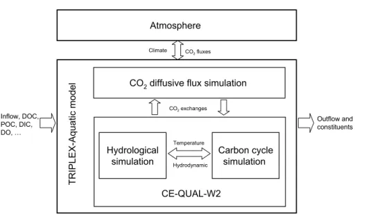
Figure 1 provides a schematic of the applied method based upon hydrological,

car-25

bon models, and CO₂ diff_{usive exchanges between air and water in the lake. The}

(6)

GMDD

6, 3509–3556, 2013

Modeling CO2

H. Wu et al.

Title Page

Tables Figures

◭ ◮

Back Close

Full Screen / Esc

Discussion

P

a

per

|

Dis

cussion

P

a

per

|

Discussion

P

a

per

|

Discussio

n

P

a

per

|

is important in modeling carbon cycle since hydrology controls physical mixing pro-cesses between spatial components, factors that can directly or indirectly control biotic and abiotic processes. The second model, the lake carbon processes focus primarily on the prediction of organic/inorganic pools via photosynthesis and respiration, and their eff_{ects on dissolved oxygen and conventional cycles of nitrogen and phosphorus.} 5

This approach represents a substantial progression in lacustrine biogeochemical mod-els since the 1970s (Harris, 1980; Beck, 1985; Ambrose et al., 1993; Kayombo et al., 2000; Chapelle et al., 2000; Omlin et al., 2001; Cole and Wells, 2006). In this paper, lake hydrodynamic and carbon simulations follow the approach of the CE-QUAL-W2 model (Cole and Wells, 2006) since the model has coupled between two-dimensional

10

hydrodynamics and carbon cycle simulations with the same time steps and spatial grid, as well as it having already been successfully applied to rivers, lakes, reservoirs, and estuaries for several decades in the past. The CE-QUAL-W2 model is available at http://www.ce.pdx.edu/w2, and its program code is not changed in this study.

The third model, the simulation of CO2diffusive fluxes at the air/water interface uses

15

a new boundary layer model developed by Cole and Caraco (1998) for lacustrine CO2

diff_{usive flux, because this simulation in CE-QUAL-W2 model was simply designed the}

gas transfer coeffi_{cient for CO}₂ _{is related to that of oxygen transfer using a factor of}

0.923 (Cole and Wells, 2006). The program code of CO2 diffusive flux submodel was

developed using the Fortran language as in the CE-QUAL-W2 model.

20

The inputs of TRIPLEX-Aquatic model and file format are same as the CE-QUAL-W2 model, including climate data (e.g. air average temperature, dew point temper-ature, wind speed and direction, cloud cover), inflow and constituent concentrations (e.g. DOC, dissolved inorganic carbon – DIC, phosphate – PO3₄−, ammonium – NH+₄, nitrate – NO−₃, and dissolved oxygen – DO), and bathymetric and geometric data of

25

lake. The model outputs represent the characteristics of hydrology (e.g. water velocity, density, temperature) and carbon processes (e.g. DOC, DIC, bicarbonates, carbon-ates, CO2concentration in water) in the lake, especially the CO2diffusive fluxes to the

(7)

GMDD

6, 3509–3556, 2013

Modeling CO2

H. Wu et al.

Title Page

Tables Figures

◭ ◮

Back Close

Full Screen / Esc

Discussion

P

a

per

|

Dis

cussion

P

a

per

|

Discussion

P

a

per

|

Discussio

n

P

a

per

|

2.1 The hydrodynamic submodel

The hydrodynamic simulation is able to characterize time variable longitudinal/vertical distributions of thermal energy in water bodies, based upon a finite diff_{erence solution}

applied to laterally averaged equations of fluid motion including momentum balance, continuity, constituent transport, free surface elevation, hydrostatic pressure, and

equa-5

tion of state (Cole and Wells, 2006) (see the Appendix A for a detail description of the model).

The model quantifies the free surface elevation, pressure, and density as well as the horizontal and vertical velocities (Cole and Wells, 2006). Explicit numerical schemes are also used to compute water velocities that aff_{ect the spatiotemporal distribution} 10

of temperature and biological/chemical constituents. The model simulates the average temperature for each model cell based upon water inflows/outflows, solar radiation, and surface heat exchanges. An equilibrium temperature approach was used to char-acterize the surface heat exchange. Spatial and temporal variations are permitted for longitudinal diff_{usion. The model computes the vertical di}ff_{usion coe}ffi_{cient from the} 15

vertical gradient of longitudinal velocities, water densities, and decay of surface wind shear. A full description of the model is off_{ered by Cole and Wells (2006).}

2.2 The carbon cycle submodel

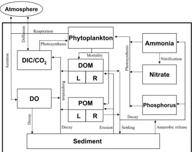
The carbon submodel explicitly depicts organic and inorganic carbon processes in lake system. The organic carbon process includes four interacting systems: phytoplankton

20

kinetics, nitrogen cycles, phosphorus cycles, and the dissolved oxygen balance (Fig. 2) (see the appendix A for a detail description of the model). The model accepts inputs in terms of diff_{erent pools of organic matter (OM) and various species of algae. OM is}

partitioned into four pools according to a combination of its physical state (dissolved – DOM versus particulate – POM) and reactivity (labile – L versus refractory – R)

char-25

(8)

GMDD

6, 3509–3556, 2013

Modeling CO2

H. Wu et al.

Title Page

Tables Figures

◭ ◮

Back Close

Full Screen / Esc

Discussion

P

a

per

|

Dis

cussion

P

a

per

|

Discussion

P

a

per

|

Discussio

n

P

a

per

|

OM (RDOM and RPOM) is less readily mineralized (i.e. having slower decay rates). All OM decay and decomposition processes in the model follow first order kinetics with temperature-dependent coeffi_{cients. The inorganic carbon processes include carbon}

dioxide input and output the inorganic carbon pool among carbonate species via two major pathways: atmospheric and biological exchange processes.

5

2.3 The CO2diffusive flux submodel

CO2 diffusion across the air/water interface (FCO₂) is driven by the concentration

gra-dient between the atmosphere and surface water and regulated by the gas exchange velocityK. Hence:

FCO₂=KCO₂(ΦCO₂−pCO2 atmKH) (1)

10

where KCO₂ is the piston velocity (cm h

−1

); Φ_CO

2 is the CO2 concentration in water

(g m−3); and (pCO2 atmKH) is the CO2concentration in equilibrium with the atmosphere. pCO2 atmrepresents the CO2partial pressure in the atmosphere, andKHis the Henry’s

constant corrected for water temperature.

KCO₂ is the piston velocity constant for CO2calculated as follows:

15

KCO₂=K600

600 ScCO₂

!n

(2)

n, the exponent, was used the value 0.5, which is appropriate for low-wind systems (Jahne et al., 1987). K₆₀₀, the piston velocity measured with SF₆ and normalized to a Schmidt number of 600, was determined according to the power function developed for low-wind speed conditions by Cole and Caraco (1998) whereU10is the wind speed

20

(m s−1) at a height of 10 m:

(9)

GMDD

6, 3509–3556, 2013

Modeling CO2

H. Wu et al.

Title Page

Tables Figures

◭ ◮

Back Close

Full Screen / Esc

Discussion

P

a

per

|

Dis

cussion

P

a

per

|

Discussion

P

a

per

|

Discussio

n

P

a

per

|

Sc_CO

2, representing the Schmidt number for carbon dioxide, is calculated according to

Eq. (4) (Wanninkhof, 1992): Sc_CO

2=1911.1−118.11TW+3.4527T

2

W−0.04132T 3

W (4)

whereTW is the water surface temperature (

◦

C).

3 Model input and test data 5

The computational grid of the two-dimensional lake model was developed based upon the bathymetric and geometric data collected from the unperturbed oligotrophic Lake Mary (46.26◦N, 76.22◦W) and Lake Jean (46.37◦N, 76.35◦W) in Qu ´ebec, Canada, with a surface area of 0.58 and 1.88 km2, respectively. The watershed areas are 1.19 km2 for Lake Mary and 5.43 km2 for Lake Jean. The region has an average

al-10

titude of 230 m, and is characterized by an average temperature of approximately 5◦C, with 1000 mm of annual precipitations. Dominant tree species are red pine and yellow birch in mature. Soils are Brunisolic Luvisols. The lake areas were divided into 24 hor-izontal segments and 10 vertical layers. Longitudinal segments were 50 m in length for Lake Mary and 160 m in length for Lake Jean. The vertical layers were 2 m thick for

15

both lakes (Fig. 3).

Time-varying boundary conditions at the surface of the lakes were set up with regard to meteorological influences. Hourly meteorological data, such as air average temper-ature, dew point tempertemper-ature, wind speed and direction as well as cloud cover were obtained from weather monitoring stations located closet to the sites (Maniwaki Airport,

20

Qu ´ebec). Daily inflow and constituent concentrations of DOM at branch – estimated by the TRIPLEX-DOC model (Wu et al., 2013) in unit multiplying the watershed forest land-scape areas of Lake Mary and Lake Jean, and adapted to TRIPLEX-Aquatic formats – were used as time-series inflow boundary conditions. Other inflow constituents – in-cluded POM, DIC, phosphate (PO3₄−), ammonium (NH+₄), nitrate (NO−₃), one species of

(10)

GMDD

6, 3509–3556, 2013

Modeling CO2

H. Wu et al.

Title Page

Tables Figures

◭ ◮

Back Close

Full Screen / Esc

Discussion

P

a

per

|

Dis

cussion

P

a

per

|

Discussion

P

a

per

|

Discussio

n

P

a

per

|

blue-green algae, and DO – were compared to data from the nearby tributary in East-ern Canada with sampled data (Wang and Veizer, 2000; H ´elie et al., 2002; H ´elie and Hillaire-Marcel, 2006; Teodoru et al., 2009) because these have not been sampled in the present study.

Hydraulic parameters governing horizontal dispersion and bottom friction were set

5

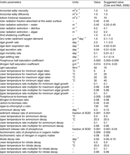
to default values using the Chezy friction model (Cole and Wells, 2006). Parameters aff_{ecting constituent kinetics are also required by the model. Initially, kinetic coe}ffi_cients

were set to default values (Cole and Wells, 2006) but subsequently tuned during the aquatic carbon process calibration so that the model output agreed with the field data. Kinetic coeffi_{cients were adjusted within acceptable ranges based upon data in} pub-10

lished literature (Table 1). Although site-specific data are preferable, the paucity of de-tails on hydraulic and kinetic coeffi_{cients in the lakes under study made it di}ffi_{cult to rely}

on site-specific data alone.

To test the model, four times campaigns were conducted in the two lakes from 2006 to 2007 because of the remote region, during periods following ice breakup in May

15

2006 (16 sampling in 6 days) and 2007 (15 sampling in 2 days), summer stratification in July 2006 (10 sampling in 2 days) and when fall overturn occurred in October 2006 (14 sampling in 3 days) for Lake Mary, and during periods in July 2006 (27 sampling in 2 days), October 2006 (1 sampling in 1 day), May 2007 (14 sampling in 1 day), July 2007 (20 sampling in 2 days) for Lake Jean. During each field trip, surface layer

20

samples and information on water temperature, dissolved CO2concentrations (pCO2)

as well as DOC at 15 cm depth was collected in pelagic sites of lake. An about 10 m depth profile of temperature, pH, DO andpCO₂was also carried out at the central point of lake.

To determinepCO2, three 30 mL water samples were collected in 60 mL

polypropy-25

lene syringes from each depth and carried out within 6 h of return to the field laboratory. They were equilibrated with an equal volume (30 mL) of ultrapure nitrogen (N2) by

(11)

GMDD

6, 3509–3556, 2013

Modeling CO2

H. Wu et al.

Title Page

Tables Figures

◭ ◮

Back Close

Full Screen / Esc

Discussion

P

a

per

|

Dis

cussion

P

a

per

|

Discussion

P

a

per

|

Discussio

n

P

a

per

|

USA). Equilibrated CO₂ concentrations in the gaseous phase were calculated accord-ing to their solubility coeffi_{cients as a function of laboratory temperature (Flett et al.,}

1976). The CO2 diffusive fluxes were therefore estimated from CO2 saturation

mea-sured in the lakes in conjunction with wind speed. DOC concentration was analyzed in 0.2 µm filtered water samples in an OI-1010 Total Carbon Analyzer (OI Analytical,

5

TX, USA) using wet persulafate oxidation. In addition, water temperature, DO, and pH profiles were taken with a YSI-6600 probe.

4 Model calibration and validation

Calibration of the TRIPLEX-Aquatic model in middle segment (the center of lake) was carried out by tuning appropriate model parameters to match the predicted and

mea-10

sured data from Lake Mary in 2007 to obtain the best possible fit within acceptable ranges specified by Cole and Wells (2006) (Table 1). The model was verified against more data measured at Lake Mary in 2006 during which it was subjected to diff_erent

ambient weather and flow conditions from those prevailing during model calibration in 2007, in order to test if the model was capable of accurately simulating the

hydrody-15

namic regime and aquatic carbon dynamics under climatic conditions diff_{ering from}

those used for calibration. The model was also validated against measurements taken in Lake Jean from 2006 to 2007. System coeffi_{cients used in the model were the same}

as those determined during model calibration. Measurements serve to validate model results related to water temperature, pH, DO,pCO2, DOC, and the CO2diffusive flux.

20

4.1 Temperature, pH, dissolved oxygen, andpCO₂

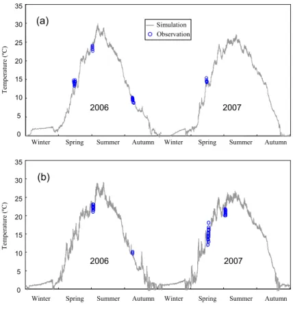
Hydrodynamic calibration is typically performed by examining vertical and longitudinal concentration gradients of conservative constituents. Cole and Wells (2006) recom-mend the use of temperature gradients as a first step for hydrodynamic calibration. The prediction of surface water temperature for 2007 was in agreement with the

(12)

GMDD

6, 3509–3556, 2013

Modeling CO2

H. Wu et al.

Title Page

Tables Figures

◭ ◮

Back Close

Full Screen / Esc

Discussion

P

a

per

|

Dis

cussion

P

a

per

|

Discussion

P

a

per

|

Discussio

n

P

a

per

|

sured data from Lake Mary (Fig. 4a) despite high variability in the calibration data. The root mean squared error (RMSE) for the calibration period was 0.9◦C. The verification of surface layer water temperature during 2006 for Lake Mary and from 2006 to 2007 for Lake Jean (Fig. 4) shows suffi_{cient agreement between the model simulations and}

field measurements. The water temperature RMSE was 1.6◦C during all simulation

5

periods in both lakes.

With regard to the validation of the vertical simulation of lake hydrodynamics and carbon cycle, the water temperature, pH, DO, and pCO₂ between model reconstruc-tions and measurements were examined. Figure 5 shows that model simulation results with respect to depth were also accordant with the recorded observations: the RMSE

10

were 0.37◦C for temperature, 0.24 for pH, 9.23 for DO (%), and 4.73 forpCO₂ during fall turnover (Fig. 5a, c, e, g), and 1.36◦C for temperature, 0.39 for pH, 11.34 for DO, and 5.55 forpCO2 during spring stratification in Lake Mary (Fig. 5b, d, f, h). However,

predicted values showed lower gradients than measured values during the spring pe-riod, especially for DO (Fig. 5f). The model also tended to underestimate water DO (%)

15

by approximately 9 % for complete profile during fall turnover (Fig. 5e).

Diff_{erences between simulated and measured DO concentration, could partly be}

ex-plained by lower tributary dissolved oxygen loads, because data was compared from the nearby tributary where may region-specific diff_{erences. For thermocline had lower}

gradients in predicted values than actual, because the stratification is a complex

in-20

tegration of multiple forcing components such as mixing rates, vertical dimensions of layer, layer temperature, basin morphometry, hydrology and, most important, meteo-rological conditions (Harleman, 1982; Owens and Effl_{er, 1989), thus, it is di}ffi_{cult to}

accurately simulate the thermocline without intensive meteorological data, while the data used in this study are measured at only one nearby meteorological station. On the

25

(13)

GMDD

6, 3509–3556, 2013

Modeling CO2

H. Wu et al.

Title Page

Tables Figures

◭ ◮

Back Close

Full Screen / Esc

Discussion

P

a

per

|

Dis

cussion

P

a

per

|

Discussion

P

a

per

|

Discussio

n

P

a

per

|

Although it is importance of water temperature and thermal stratification dynamics for temporal variation of surface water CO₂ in boreal lake (Aberg et al., 2010), the RMSE of surface temperature,pCO2in model simulation lead to approximately 12 %

and 15 % mean errors in CO2diffusive flux respectively, they had only minor impacts

on lake CO₂ emission. In general, these results suggest that the model reasonably

5

represented surface and vertical variations of water temperature, pH, DO,pCO2 and

hydrodynamics of the lake system.

4.2 Dissolved organic carbon

Dissolved organic carbon, a substrate for microbial respiration, is a key constituent in aquatic carbon dynamics and could be the source of significant variations in lake

10

pCO2 (Hope et al., 1996; Sobek et al., 2003). Figure 6 offers a comparison between

simulated and observed daily DOC concentrations from 2006 to 2007 in Lake Mary. Simulated values were reasonably distributed in the middle of the observational period (RMSE=_{0.7). This agreement obtained during 2006 demonstrates that the model is}

capable of modeling DOC carbon-process properties within Lake Mary.

15

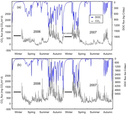
4.3 CO2diffusive flux

In this study, a zero CO2 flux was assumed during the ice cover period for the

simu-lations. During the ice-free period, there were considerable seasonal variations in the magnitude of the CO₂ diff_{usive flux and a distinct seasonal cycle in both Lake Mary}

and Lake Jean (Fig. 7). Peak fluxes occurred in the month of May following ice breakup

20

and reached a brief, temporary minimum in early July. This minimum was followed by a second peak in late fall associated with autumnal mixing.

In comparing simulated results with observational daily data from 2006 for Lake Mary and from 2006 to 2007 for Lake Jean, the model successfully reproduced the observed distributions of CO₂ flux in both lakes, except for a daily value in autumn 2006 in Lake

25

(14)

measure-GMDD

6, 3509–3556, 2013

Modeling CO2

H. Wu et al.

Title Page

Tables Figures

◭ ◮

Back Close

Full Screen / Esc

Discussion

P

a

per

|

Dis

cussion

P

a

per

|

Discussion

P

a

per

|

Discussio

n

P

a

per

|

ments were absent in this study, such reasonable agreement between simulated and observed hydrodynamic plots and aquatic carbon dynamic parameters demonstrates that TRIPLEX-Aquatic was able to model various hydrodynamic and aquatic carbon cycle processes within the lake systems. It can thus be applied to simulate the CO2

diff_{usive flux for lakes.} 5

5 Terrestrial DOC and lake CO2emissions

5.1 Seasonal and annual mean lake CO2diffusive flux

The most current estimates of the annual CO2emission budgets of lakes, based upon

measurements, only consider CO2 produced during ice-free periods. However, CO2

produced during winter months may accumulate under the ice cover and be

subse-10

quently released into the atmosphere once ice break-up occurs in spring (Striegl et al., 2001; Duchemin et al., 2006; Demarty et al., 2011). This early spring CO2 release

accumulated during the winter should be accounted for in order to develop a more realistic annual CO2emission budget for boreal lakes.

At the end of the winter season, the TRIPLEX-Aquatic model was well-calibrated to

15

capture the principal characteristics of a high CO₂flux episode just after ice melt over a period of approximately ten days (Fig. 7a, b). During this period the model estimated that approximately 80 % of the CO2 contained in the water column of Lake Mary and

Lake Jean was emitted into the atmosphere. The values for early spring CO₂emissions ranged from 5 % to 8 % of the annual CO2 diffusive emission budget for both lakes

20

during the 2006 and 2007 period, which are thus an important portion in the annual CO₂budget.

For Lake Mary and Lake Jean, variations in daily CO2 flux were greatest during

spring and fall and smallest during summer stratification (Fig. 7a, b). The average sum-mer (from July to August) values were approximately 24–88 % lower than the average

(15)

GMDD

6, 3509–3556, 2013

Modeling CO2

H. Wu et al.

Title Page

Tables Figures

◭ ◮

Back Close

Full Screen / Esc

Discussion

P

a

per

|

Dis

cussion

P

a

per

|

Discussion

P

a

per

|

Discussio

n

P

a

per

|

calculated values for the entire open water period in both lakes, a typical situation for northern temperate dimictic lakes (Hesslein et al., 1990).

Although there is a reasonable agreement between model simulations and field mea-surements for daily CO2 diffusive flux (Fig. 7), when comparisons are based on

sea-sonal CO₂diff_{usive flux in Lake Mary (Fig. 8a), it was noted that the observations made} 5

during the autumn of 2006 were much higher than those in the simulation. For Lake Jean (Fig. 8b) measurements taken in the summer of 2006 were lower than those in the model simulations.

In respect to the annual mean CO2 diffusion during the open water period in 2006,

the simulated value was 447 mg CO2m

−2

day−1in Lake Mary, broadly consistent with

10

the measured value of 493 mg CO2m

−2

day−1. In Lake Jean the simulated annual mean CO₂ emission was 589 mg CO₂m−2day−1, significantly higher than the measurement of 360 mg CO2m

−2

day−1taken during the same period.

5.2 Impact of terrestrial DOC on lacustrine CO2diffusive emissions

A large body of literature suggests net heterotrophy is the key factor responsible for

15

the often observed supersaturation of CO₂ in lake systems (del Giorgio et al., 1999; Cole et al., 2000; Jonsson et al., 2001, 2003; Prairie et al., 2002; Algesten et al., 2003; Hanson et al., 2003, 2004; Sobek et al., 2003; Karlsson et al., 2007; McCallister and del Giorgio, 2008), but this inference is tempered by uncertainties in the magnitude of the carbon load to lakes, and the relative contributions to lake CO₂emission (Hanson

20

et al., 2004; Karlsson et al., 2007; McCallister and del Giorgio, 2008).

To evaluate impacts of terrestrial DOC on the lake CO2 emission regime, a

com-parison between DOC inputs and CO₂ fluxes was performed where the DOC data was simulated by way of the TRIPLEX-DOC model. Figure 9 shows a positive re-lationship between terrestrial DOC and CO2 flux in both Lake Mary (CO2 flux=

25

(16)

GMDD

6, 3509–3556, 2013

Modeling CO2

H. Wu et al.

Title Page

Tables Figures

◭ ◮

Back Close

Full Screen / Esc

Discussion

P

a

per

|

Dis

cussion

P

a

per

|

Discussion

P

a

per

|

Discussio

n

P

a

per

|

R=_0.63,_{P <}_{0.0001), underlining the important role of DOC inputs in seasonal CO}₂

diff_{usive flux variations.}

To further estimate the impact of terrestrial DOC on aquatic CO2diffusive flux, a

sen-sitivity analysis was carried out on the modeled results for 2006 to 2007 for both lakes by setting the terrestrial DOC inputs to zero while keeping other variable inputs at

5

normal values, mimicking a situation in which the terrestrial DOC input would be nil. Results showed the annual mean CO₂ diff_{usive flux from lakes under no-DOC-input}

conditions were much lower (approximately 30–45 % lower) than values with DOC in-puts (Fig. 10a, b).

6 Discussion and conclusion

10

6.1 Comparison model with earlier approaches

There are presently only a handful of model studies (Hanson et al., 2004; Cardille et al., 2007; Buff_{am et al., 2011) that have tried to link terrestrial watershed carbon inputs to}

their aquatic components for CO2 emission. However, integration is still pending. In

this study a comprehensive process-based aquatic carbon model (TRIPLEX-Aquatic)

15

incorporating both terrestrial inputs, an aquatic carbon cycle, and detailed hydrody-namic simulation was developed and applied to investigate aquatic CO2 diffusion in

lake ecosystems within Qu ´ebec, Canada.

Although recent lake carbon models (Hanson et al., 2004; Cardille et al., 2007) in-tegrate inputs of terrestrial DOC from watersheds, such models have no or very low

20

hydrodynamic spatial resolution. In addition, these models do not include real-time me-teorological conditions, while using constants to represent physical mixing processes between spatial components. The mass balance model (Jones et al., 2009) accounts for real-time metrological data for lake carbon simulation, but does not include inputs of terrestrial DOC from catchments. Accordingly, the lake hydrodynamic routine is less

25

(17)

GMDD

6, 3509–3556, 2013

Modeling CO2

H. Wu et al.

Title Page

Tables Figures

◭ ◮

Back Close

Full Screen / Esc

Discussion

P

a

per

|

Dis

cussion

P

a

per

|

Discussion

P

a

per

|

Discussio

n

P

a

per

|

estimates are based upon empirical models whereas simulations in this study were based on a process-based model.

A previous numerical CO2emission model developed by Barrette and Laprise (2002)

illustrate the relevant approach to modeling physical processes in the water column based upon an extension of the lake water column model. It was used to study the

5

temporal and spatial distribution of the dissolved CO2 concentration profile and the

CO2 diffusive flux at the air/water interface. However, this particular model does not

include the autotrophic and heterotrophic production of organic matter based upon variables such as water temperature, dissolved oxygen, nutrient salts, and terrestrial organic matter from catchments. All were included in the model used in the present

10

study.

For the CO2diffusive flux submodel in TRIPLEX-Aquatic model, although a few

stud-ies have indicated that CO2 diffusive fluxes obtained with the boundary layer

tech-nique might have been underestimated (Anderson et al., 1999; Jonsson et al., 2008) in comparison with the eddy covariance technique that is a direct measurement of the

15

CO2 flux, while the studies of Eugster et al. (2003) and Vesala et al. (2006) showed

a good agreement. The boundary layer model of Cole and Caraco (1998) has also been validated and provides accurate or no bias estimations of CO2evasion over most

of the sampling intervals based on the dry ice sowing experiment in a small boreal oligotrophic lake in Quebec, Canada (Soumis et al., 2008), and whole-lake sulfur

hex-20

aflouride (SF₆) additions in temperate lakes near Land O’Lake, WI, USA (Cole et al., 2010) under a low-wind environment which is similar to the lakes in this study. Even though the Cole and Caraco (1998) model in this study is relatively simple, it is reason-able for estimating the CO₂diff_{usive flux, partly because there has been little evidence}

that incorporation of comprehensive surface forcing provides a better flux field than

25

(18)

GMDD

6, 3509–3556, 2013

Modeling CO2

H. Wu et al.

Title Page

Tables Figures

◭ ◮

Back Close

Full Screen / Esc

Discussion

P

a

per

|

Dis

cussion

P

a

per

|

Discussion

P

a

per

|

Discussio

n

P

a

per

|

6.2 Impact of terrestrial DOC on CO2emission

Based on model validation, the agreement between observations and simulated results indicates the model is able to capture the principal hydrological characteristics and carbon dynamic processes in lake systems, it thus provides a realistic CO2 diffusive

flux simulation.

5

For the early spring CO₂ emissions, our model can successfully simulate the high CO2flux episode following ice breakup events. Such emission peaks were also

identi-fied by measurements in boreal lakes (Riera et al., 1999; Duchemin et al., 2006; Huotari et al., 2009; Demarty et al., 2011). Duchemin et al. (2006) estimated during the week following ice breakup 95 % of the dissolved CO₂ contained in the water column was

10

released into the atmosphere. CO2emitted during this short period would account for

7–52 % of total annual emissions (Duchemin et al., 2006; Huotari et al., 2009; Demarty et al., 2011). Our results are within the lower end of their estimates, and reveal a sig-nificant CO2contribution during the ice break-up periods to the annual CO2budget of

aquatic ecosystems in boreal lakes.

15

Concerning the seasonal and annual CO₂emission, the diff_{erences between}

simu-lated and measured CO2diffusive flux values may result, in part, from the absence of

systematic (or continuous) measurements of highly variable daily emissions: there are only a few daily observations for each season and these cannot accurately represent the natural CO2 emission, thus resulting in a substantial overestimation or

underesti-20

mation of seasonal, or annual flux values. On one hand, for the analysis of seasonal or annual variability, we should, in the future, use the eddy covariance measurements, which provide more frequent sampling and more accurate estimates of the CO2

emis-sion (Vesala et al., 2006; Jonsson et al., 2008; Huotari et al., 2011). On the other hand, it is our hope that the model simulation could contribute to the development of more

25

eff_{ective sampling strategies, based on the characteristics of the simulated temporal}

(19)

GMDD

6, 3509–3556, 2013

Modeling CO2

H. Wu et al.

Title Page

Tables Figures

◭ ◮

Back Close

Full Screen / Esc

Discussion

P

a

per

|

Dis

cussion

P

a

per

|

Discussion

P

a

per

|

Discussio

n

P

a

per

|

For the impact of terrestrial DOC on lake CO₂emission, results from this study re-veal that approximately 30–45 % of the annual CO2 diffusive flux is due to terrestrial

DOC input. Our study agree with the work ranged from 3 % to 70 % CO2 flux from

terrestrial organic carbon based on theδ13C measurement in lakes of southern Que-bec, Canada (McCallister and del Giorgio, 2008), and consistent with the estimates

5

between 30 % and 80 % of organic carbon exported from the watershed was released to the atmosphere CO2in lakes in the boreal Scandinavia (Algesten et al., 2003). The

fate of terrestrial DOC in this study is also in the same range as the modeled estimates approximately 40–52 % respiration was supported by allochthonous DOC in Wisconsin lakes (Cole et al., 2002; Hanson et al., 2004). Our results thus support the hypothesis

10

that a significant fraction of aquatic CO₂ diff_{usive flux is attributable to allochthonous}

organic carbon inputs from lake catchments (del Giorgio et al., 1999; Cole et al., 2000, 2007; Jonsson et al., 2001, 2003; Prairie et al., 2002; Algesten et al., 2003; Hanson et al., 2003, 2004; Karlsson et al., 2007; McCallister and del Giorgio, 2008; Battin et al., 2009; Buff_{am et al., 2011).}

15

There is generally a net uptake of CO2from the atmosphere in boreal forests (Chapin

III et al., 2000; Dunn et al., 2007), whereas, lake ecosystems seems to process a large amount of terrestrial derived primary production and alter the balance between car-bon sequestration and CO2 release. It demonstrates that lake ecosystems contribute

significantly to regional carbon balances.

20

6.3 Future improvements to the TRIPLEX-Aquatic model

A major challenge for developing a new process-based model is the validation phase. Results presented in this study demonstrate that the TRIPLEX-Aquatic model is able to provide reasonable simulations of hydrodynamic and carbon processes in two selected boreal oligotrophic lakes (Lake Mary and Lake Jean). However, additional system

veri-25

(20)

GMDD

6, 3509–3556, 2013

Modeling CO2

H. Wu et al.

Title Page

Tables Figures

◭ ◮

Back Close

Full Screen / Esc

Discussion

P

a

per

|

Dis

cussion

P

a

per

|

Discussion

P

a

per

|

Discussio

n

P

a

per

|

In addition, the aquatic carbon approach is relatively simple in the current version of TRIPLEX-Aquatic. Decomposition processes of organic carbon follow first order ki-netics of temperature-dependent coeffi_{cients for bacterial degradation. In fact,}

miner-alization of allochthonous organic carbon occurs primarily, if not exclusively, by way of bacterial degradation (Jonsson et al., 2001). Photochemical degradation (Gran ´eli

5

et al., 1996) and its interaction with bacterial mineralization (Bertilsson and Tranvik, 1998) may add substantially to overall lake mineralization. Moreover, groundwater in-flow (Kling et al., 1991; Striegl and Michmerhuizen, 1998) and surface water (Dillon and Molot, 1997; Cardille et al., 2007) enriched in inorganic carbon derived from weathering and soil respiration could be an important factor in some lakes.

10

There is also increasing evidences that gas transfer near the air/water interface can-not be adequately quantified using wind speed alone (Wanninkhof et al., 2009; Mac-Intyre et al., 2010). Studies have shown that other factors, such as friction velocity, bubbles, buoyancy, energy dissipation, fetch, surface slicks, rain, and chemical en-hancement (Asher and Pankow, 1986; Wallace and Wirick, 1992; Erickson III, 1993;

15

Ho et al., 2000; Zappa et al., 2001; McNeil and d’Asaro, 2007; Wanninkhof et al., 2009; MacIntyre et al., 2010), can also aff_{ect the gas transfer velocities. Disregarding these}

factors will undoubtedly add to the analytical uncertainty in relation to the aquatic car-bon cycle. These shortcomings will be addressed and minimized in the future.

It is important to point out that the TRIPLEX-Aquatic model, incorporating robust

20

process-based hydrodynamic components, could be feasibly adapted to reservoirs in the future in spite of the fact that their hydrodynamic and biogeochemical characteris-tics diff_{er from those observed in lake systems. The model can also be coupled with}

land surface and ecosystem models at various horizontal resolutions or forced with GCM outputs to investigate the potential impact of climate and land use changes on

25

(21)

GMDD

6, 3509–3556, 2013

Modeling CO2

H. Wu et al.

Title Page

Tables Figures

◭ ◮

Back Close

Full Screen / Esc

Discussion

P

a

per

|

Dis

cussion

P

a

per

|

Discussion

P

a

per

|

Discussio

n

P

a

per

|

Appendix A

A1 The hydrodynamic submodel

The hyrodynamic simulation follows the approaches of CE-QUAL-W2 (Cole and Wells, 2006). The equations of fluid motion include: (1) momentum balance (Eq. A1); (2)

con-5

tinuity (Eq. A2); (3) constituent transport (Eq. A3); (4) free surface elevation (Eq. A4); (5) hydrostatic pressure (Eq. A5); and, (6) equation of state (Eq. A6)

∂UB ∂t +

∂UUB ∂x +

∂W UB ∂z =−

1

ρ ∂BP

∂x +

∂(BAx∂U_∂x)

∂x + ∂Bτ_x

∂z (A1)

∂UB ∂x +

∂W B

∂z =qB (A2)

∂BΦ

∂t +

∂UBΦ

∂x +

∂W BΦ

∂z −

∂(BD_x∂_∂xΦ)

∂x −

∂(BD_z∂_∂zΦ)

∂z =qΦB+SΦB (A3)

10

∂B_ηη

∂t = ∂ ∂z

h Z

η

UBdz−

h Z

η

qBdz (A4)

∂P

∂z =ρg (A5)

ρ=_f₍_T_W_,Φ_TDS_,Φ_SS₎ _(A6)

whereU andW are the laterally averaged velocity components (m s−1) in eachxandz

15

direction;Bis the water body width (m);tis the time (s);ρis the water density (kg m−3);

P is the pressure (N m−2);Axis the momentum dispersion coefficient (m

2

(22)

GMDD

6, 3509–3556, 2013

Modeling CO2

H. Wu et al.

Title Page

Tables Figures

◭ ◮

Back Close

Full Screen / Esc

Discussion

P

a

per

|

Dis

cussion

P

a

per

|

Discussion

P

a

per

|

Discussio

n

P

a

per

|

concentration (g m−3);Dx andDz are the temperature and constituent dispersion

coef-ficients in eachx and z direction; qΦ is the lateral boundary inflow and outflow mass

flow rate of the constituent (g m−3s−1);SΦ is the kinetics source/sink term for the

con-stituent concentrations (g m−3s−1); B_η is the time and spatially varying surface width (m);ηis the free water surface location (m); his the total depth (m);g is the

gravita-5

tional acceleration (m s−2); andf(TW,ΦTDS,ΦSS) is the density function dependent on

water temperature (◦C), total solids or salinity, and suspended solids.

A2 The carbon cycle submodel

The organic carbon cycle includes phytoplankton kinetics, nitrogen cycles, phosphorus cycles, and the dissolved oxygen balance (Cole and Wells, 2006).

10

A2.1 Phytoplankton

Photosynthesis is the primary ecosystem process and the basis of carbon dynamics in aquatic ecosystems. The phytoplankton growth rate (Kg, in day

−1

) is estimated as a function of temperature (T, in◦C), light intensity (I, in W m2), and concentrations of limiting nutrients (g m−3) such as nitrogen (N) and phosphorus (P).

15

Kg=K

∗

gf(T)f(I)f(N, P) (A7)

whereKg∗is the maximum growth rate (day

−1

). An asymmetric function is used to simu-late the influence of temperature on phytoplankton biological processes (Thornton and Lessem, 1978). This function depicts an optimum range of temperature (fromT₂toT₃) for biological process rates that decrease asymmetrically at lower (T1) and higher (T4)

(23)

GMDD

6, 3509–3556, 2013

Modeling CO2

H. Wu et al.

Title Page

Tables Figures

◭ ◮

Back Close

Full Screen / Esc

Discussion

P

a

per

|

Dis

cussion

P

a

per

|

Discussion

P

a

per

|

Discussio

n

P

a

per

|

temperatures.

f(T)=₀ _if _T ≤T1 (A8)

f(T)= K1e γ_r(T−T₁)

1+_K₁_eγ_r(T−T₁)₋_K 1

K4e

γ_f(T₄−T)

1+_K₄_eγ_f(T₄−T)₋_K 4

if T₁< T < T₂ (A9)

f(T)=₀ _if _T ≥T4 (A10)

5

where

γ_r= 1

T₂−T₁ln

K2(1−K1) K1(1−K2)

(A11)

γ_f= 1

T₄−T₃ln

K3(1−K4) K4(1−K3)

(A12)

Compared to most other temperature functions with a single optimum value reported

10

in existing literature (Zeng et al., 2006), this function combines two logistic equations to describe the rising (γ_r) and falling (γ_f) limb temperature multipliers.

The light function is described by Steels’s (1965) according to the equation below:

f(I)= I

IS

e(1−II_S) _(A13)

whereIS is the saturating light intensity (W m

−2

), andIis the available light intensity at

15

depthz (m):

I=₍₁−β)I0e

−αz

(A14)

I0 is the light intensity at the water surface (W m

−2

);βis the fraction of solar radiation absorbed at the water surface; andαis the light extinction coeffi_{cient, a combination of}

(24)

GMDD

6, 3509–3556, 2013

Modeling CO2

H. Wu et al.

Title Page

Tables Figures

◭ ◮

Back Close

Full Screen / Esc

Discussion

P

a

per

|

Dis

cussion

P

a

per

|

Discussion

P

a

per

|

Discussio

n

P

a

per

|

Nitrogen and phosphorus are the most important modeled limiting nutrients (Ambrose et al., 1993). Their concentrations are calculated based upon the Michaelis– Menten or Monod relationships that assume the nutrient composition of algal cells remains constant, and the external concentrationsΦ _{(g m}−3_{) of available nutrients (}_i₎

aff_{ect algal growth rates by a factor of:} 5

f(P, N)= Φi

P_i+ Φ_i (A15)

wherePi is the half-saturation constant for nutrienti (g m

−3

). The rate equation for each algal group are:

∂Φ

∂t =KgΦ−KrΦ−KeΦ−KmΦ−ω ∂Φ

∂z (A16)

K_r=_K∗

rf(T) (A17)

10

K_e=₍₁−f(I))f(T)K_e∗ (A18) Km=f(T)K

∗

m (A19)

where Kg, Kr, Ke, Km, and ω are algal growth, dark respiration, excretion, mortality

(s−1), and the settling rate (m s−1), respectively.Φ_{is the algal concentration (g m}−3_);_z 15

is the cell height (m);Kr∗,K

∗

e, andK

∗

mare the maximum dark respiration, excretion, and

mortality rate (s−1), respectively.

A2.2 Nitrogen cycle

Three variables are used to characterize the nitrogen cycle: organic nitrogen, ammo-nium, and nitrate. As phytoplankton proliferates, dissolved inorganic nitrogen is taken

20

(25)

GMDD

6, 3509–3556, 2013

Modeling CO2

H. Wu et al.

Title Page

Tables Figures

◭ ◮

Back Close

Full Screen / Esc

Discussion

P

a

per

|

Dis

cussion

P

a

per

|

Discussion

P

a

per

|

Discussio

n

P

a

per

|

The rate equations of nitrogen in labile and refractory dissolved organic matter are:

∂Φ_LDOM-N

∂t =

X

KeδNΦa+ X

(1−Pm)KmδNΦa−KLDOMγOMΦLDOM-N −KL→RγOMΦLDOM-N

(A20)

∂Φ_RDOM-N

∂t =KL→RΦLDOM-N−γOMKRDOMΦRDOM-N (A21)

whereKeand Km are the algal excretion and mortality rates (s

−1

), and δNis the algal

5

stoichiometric coeffi_{cient for nitrogen;} Φ_a_, Φ_LDOM-N_{, and} Φ_RDOM-N _{are algal, liable,}

and refractory DOM nitrogen concentrations (g m−3), respectively; Pm is the pattern

coeffi_{cient for algal mortality, and}_K_LDOM_and_K_RDOM_{are the labile and refractory DOM}

decay rates (s−1);γ_OM is the temperature rate multiplier for organic matter decay, and

KL→Ris the labile to refractory DOM transfer rate (s

−1

).

10

For nitrogen in labile and refractory particulate organic matter:

∂Φ_LPOM-N

∂t =

X

PmKmδNΦa−KLPOMγOMΦLPOM-N−KL→RΦLPOM-N

−ωPOM

∂Φ_LPOM-N

∂z

(A22)

∂Φ_RPOM-N

∂t =KL→RΦLPOM-N−γOMKRPOMΦRPOM-N−ωPOM

∂Φ_RPOM-N

∂z (A23)

whereKLPOMand KRPOM are the labile and refractory POM decay rates (s

−1

),

respec-15

tively;KL→Ris the labile to refractory POM transfer rate (s

−1

);ωPOMis the POM settling

rate (m s−1); and Φ_LPOM-N _and Φ_RPOM-N _{are the liable and refractory POM nitrogen}

(26)

GMDD

6, 3509–3556, 2013

Modeling CO2

H. Wu et al.

Title Page

Tables Figures

◭ ◮

Back Close

Full Screen / Esc

Discussion

P

a

per

|

Dis

cussion

P

a

per

|

Discussion

P

a

per

|

Discussio

n

P

a

per

|

For ammonium (NH4): ∂Φ_NH

4

∂t =

X

KrδNΦS− X

KgδNΦaPNH₄+ 4 X

i=1

KiδNOMγOMΦi+KSδNOMγOMΦS

+X_K_CBOD_R_CBOD_δ_N-CBODΘT−20_Φ

CBOD+KNO_xγNO_xΦNO_x−KNH₄γNH₄ΦNH₄

(A24)

whereKi (i =1, 2, 3, 4) are the labile and refractory DOM and the labile and

refrac-tory POM decay rates (s−1), respectively;K_S,K_CBOD,K_NO

x, andKNH4 are the sediment,

5

CBOD, nitrate-nitrogen, and ammonium decay rates (s−1), respectively;δN,δNOM, and δN-CBOD are the algal, organic matter, and CBOD stochiometric coefficients for

nitro-gen, respectively;Φ_S_,Φ_a_,Φ_CBOD_,Φ_NO

x, and ΦNH4 are the organic sediment, algal,

CBOD, nitrate-nitrogen, and ammonium concentrations (g m−3), respectively;Φ_i ₍_i =_1,

2, 3, 4) are the labile and refractory DOM and the labile and refractory POM

concentra-10

tions (g m−3), respectively;γOM,γNO_x, andγNH₄ are the temperature rate multipliers for

organic matter decay, denitrification, and nitrification, respectively;Θ_{is the temperature}

rate multiplier for CBOD decay; andPNH₄ is the ammonium preference factor expressed

as:

PNH₄=ΦNH₄

Φ_NO

x

K_NH

4+ ΦNH4 KNH4+ ΦNOx

+ Φ_NH

4

KNH₄

Φ_NH

4+ ΦNOx KNH4+ ΦNOx

(A25)

15

For nitrite-nitrate:

∂Φ_NO

x

∂t =KNH4γNH4ΦNH4−KNOxγNOxΦNOx−ωNOx

∂Φ_NO

x

∂z −

X

KgδNΦa(1−PNH₄) (A26)

whereωNO_x is the sediment transfer velocity (m s

−1

(27)

GMDD

6, 3509–3556, 2013

Modeling CO2

H. Wu et al.

Title Page

Tables Figures

◭ ◮

Back Close

Full Screen / Esc

Discussion

P

a

per

|

Dis

cussion

P

a

per

|

Discussion

P

a

per

|

Discussio

n

P

a

per

|

A2.3 Phosphorus cycle

Phosphorus is an important element in aquatic ecosystems since it serves as one of the primary nutrients in phytoplankton growth (Carlson, 1977; Carpenter et al., 1998). Phosphorus is assumed to be completely available for phytoplankton as orthophos-phate. It, however, becomes unavailable when it is removed through adsorption by way

5

of suspended sediment particles and iron.

∂Φ_P

∂t =

X

(K_r−K_g)δ_PΦ_a+ 4 X

i=1

K_iδ_POMγ_OMΦ_i+_K_S_δ_POM_γ_OMΦ_S

+X_K_CBOD_R_CBOD_δ_P-CBODΘT−20_Φ CBOD−

(P

ωISSΦISS+ωFeΦFe)PP

∆_z ΦP

(A27)

where δP, δPOM, and δP-CBOD are the algal, organic matter, and phosphorus/CBOD

stochiometric coeffi_{cients for phosphorus, respectively;}_ω_ISS_{, and}_ω_Fe_{are the inorganic} 10

suspended solids and particulate organic matter settling velocities (m s−1);Φ_ISS_,Φ_Fe_,

andΦ_P _{are the inorganic suspended solids, particulate organic matter, and}

phospho-rous concentrations (g m−3), respectively; and∆_z _{is the model cell thickness (m).}

A2.4 Dissolved oxygen balance

Oxygen is one of the most important elements in aquatic ecosystems. Dissolved

oxy-15

gen (DO) concentrations depend upon exchanges with the atmosphere, consumption through algal respiration, production by algal photosynthesis, biochemical oxygen de-mand (BOD) decay, nitrification, and sediment organic matter decay.

∂Φ_DO

∂t =

X

(Kg−Kr)δOMΦa+AsurKL(Φ

′

DO−ΦDO)− 4 X

i=₁

KiδOMγOMΦi

−K_Sδ_OMγ_OMΦ_S−XK_CBODR_CBODΘT−20Φ_CBOD−K_NH

4δNH4γNH4ΦNH4

(A28)