Key words: network models, integer programming, Karush-Kuhn-Tucker, transportation.
Palavras-Chave: modelos de rede, programação inteira, Karush-Kuhn-Tucker, transportes.
Recommended Citation Resumo
Os modelos de rede e programação inteira são uma variedade bem conhecida de problemas de tomada de decisão. Uma área muito útil e difundida de aplicação é o uso e gestão eficiente de recursos escassos para aumentar a produtividade. Estas aplicações incluem problemas operacionais como a distribuição de mercadorias, programação de produção e sequenciamento de máquinas e problemas de planejamento, como a alocação de orçamento de capital de instalações, seleção de portfolios, e problemas de desenho de redes de telecomunicações e transportes. O problema do transporte, que é um dos problemas da rede de programação inteira, é um problema que lida com a distribuição de qualquer bem de qualquer grupo de 'fontes' para qualquer grupo de destinos ou na forma mais efetiva em custos, dadas restrições de 'oferta' e de 'demanda'. Dependendo da natureza da função de custo, o problema do transporte pode ser categorizado em problemas de transporte linear e não linear. Neste artigo é aplicado o algoritmo de otimização Karush-Kuhn-Tucker (KKT) para resolver o problema de transportes com volume de descontos para um operador logístico em Gana.
Mubashiru, A-S. S. (2014) Transportation with volume discount - a case study of a logistic operator in Ghana. Journal of Transport Literature, vol. 8, n. 2, pp. 7-37.
Abdul-Salam Sibidoo Mubashiru*
Abstract
Network models and integer programming are well known variety of decision making problems. A very useful and widespread area of application is the management and efficient use of scarce resources to increase productivity. These applications include operational problems such as the distributions of goods, production scheduling and machine sequencing, and planning problems such as capital budgeting facility allocation, portfolio selection, and design problems such as telecommunication and transportation network design. The transportation problem, which is one of network integer programming problems is a problem that deals with distributing any commodity from any group of 'sources' to any group of destinations or 'sinks' in the most cost effective way with a given 'supply' and 'demand' constraints. Depending on the nature of the cost function, the transportation problem can be categorized into linear and nonlinear transportation problem. We applied Karush-Kuhn-Tucker (KKT) optimality algorithm to solve our problem of transportation with volume discount for a logistic operator in Ghana.
This paper is downloadable at www.transport-literature.org/open-access.
■JTL|RELIT is a fully electronic, peer-reviewed, open access, international journal focused on emerging transport markets and published by BPTS - Brazilian Transport Planning Society. Website www.transport-literature.org. ISSN 2238-1031.
* Email: [email protected].
Research Directory
Submitted 24 Jan 2013; received in revised form 17 Apr 2013; accepted 18 Oct 2013
Transportation with volume discount
- a case study of a logistic operator in Ghana
[Transporte com desconto de volume - um estudo de caso de um operador logístico em Gana]
Kwame Nkrumah University of Science and Technology, Ghana
Introduction
This paper seeks to solve a transportation problem with volume discount. The costs of goods
are determined by factors such as: the costs of raw materials, labour, and transport. When cost
of raw materials rises, so does the cost of the goods. Transportation cost also affects the
pricing system. It is assumed that the cost of goods per unit shipped from a give source to a
given destination is fixed regardless of the volume shipped. But in actuality the cost may not
be fixed. Volume discounts are sometimes available for large shipments so that the marginal
costs of shipping one unit might follow a particular pattern. Our focus will be to develop a
mathematical model using optimization techniques to close the demand and supply gap by
discounting so as to minimize total transportation cost.
This research seeks to apply the existing general nonlinear programming algorithms to solve
our problem. The research strategy that the study will utilize is the descriptive method. In this
study, primary and secondary research will be both incorporated. The reason for this is to be
able to provide adequate discussion for the readers that will help them understand more about
the issue and the different variables that involve with it. The primary data for the study will be
represented by the survey results that will be acquired from the respondents. On the other
hand, the literature reviews to be presented in the second Section of the study will represent
the secondary data of the study. The secondary sources of data will come from published
articles from books, journals, theses and related literature. Different algorithms to the various
transportation problems will be presented.
Until recently, heavy trucks could load up to any capacity without limit. These trucks
normally exceed the average loading capacity of the truck. This was partially due to high
transportation cost. Drivers and transport owners together with transport users had to find a
way of compensating for the high cost of transport by increasing the truck load so as to
maximize profit. This had ripple effect on the state as a whole: increase road accidents,
destruction of roads, pressure is also put on the vehicle, and longer time being spent on the
road before getting destination. There is also the effect of increased cost of goods thereby
to the problems. There is therefore the need to determine the maximum loading capacity of
trucks.
The purpose of this work is to find out whether given volume discounts on transportation
costs could minimize total transportation cost thereby increasing total revenue of producers
and retailers as well as solving some of the aforementioned problems associated with
transportation.
This paper is organized in the following way. In Section 1, we presented a background study
of transportation problem, objectives, methodology, justification and limitations of the study.
In Section 2, related works in the field of transportation problems will be discussed. Section 3
presents various existing algorithms for solving the various transportation problems. Section 4
presents data collection and analysis of the study. And finally, we present the conclusions and
recommendations of the study.
1. Background
Contemporary research in logistics management relies on an increased recognition that an
integrated plan requires coordinating different functional specialties within a system in
keeping with this trend; we focus on the integration of production, inventory and
transportation arising in a supplier- retailer logistic system. In the general inventory models,
costs of such issues are usually accounted according to the following assumptions: the
production cost is proportional to the quantity of products produced. The ordering cost, which
refers to the charge for preparing of production, is independent of the quantity ordered. The
inventory cost (shortage cost) is proportional to the quantity of products stored (out of order)
as well as the duration for which these items are stored (stock out). When products are
delivered from the supplier to the consumer, transportation costs are incurred. In the
traditional economic order quantity (EOQ) model, the transportation cost is calculated
together with the production cost, or with the ordering cost. However, in a practical logistic
system, the transportation cost of a vehicle includes both of the fixed cost and the variable
cost. The fixed cost, which is considered to be a constant sum in each period, refers to some
necessary expenses such as parking fare and rewards to the driver. As to the variable cost, it
short, considering the real condition, it is unreasonable to assume that the transportation cost
is proportional to the quantity delivered or is a constant sum.
Transportation models provide a powerful framework to meet this challenge. They ensure the
efficient movement and timely availability of raw materials and finished goods.
Transportation problem is a linear programming problem stemmed from a network structure
consisting of a finite number of nodes and arcs attached to them. When the transportation plan
is made up, the volume discounts brought by large quantities of transportation should not be
pursuited excessively. As this would bound to increase inventory costs throughout the system,
also when the inventory strategy is determined, transportation costs cannot be dealt with as a
fixed fee, but as a variable cost directly impacting on transportation frequency and inventory
distribution. Under the prerequisite of comprehensively balancing the transportation costs and
inventory costs, the objectives that Inventory-Transportation Integrated Optimization problem
(ITIO) are to optimize the logistics system, reduce logistics costs, and determine the
transportation program and inventory strategy of the system.
One of the earliest and most fruitful applications of linear programming techniques has been
the formulation and solution of the transportation problems as a linear programming problem.
The basic transportation problem was originally developed by Hitchcock (1941). The
objective of the transportation problem is to determine the optimal amounts of a commodity
to be transported from various supply points to various demand points so that the total
transportation cost is a minimum. The unit costs i.e. the cost of transporting one unit from a
particular supply point to a particular demand point, the amounts available at the supply
points and the amounts required at the demand points are the parameters of the transportation
problem.
Industrial development today depends on the efficiency of the transportation and logistics
activities. Transportation can be described as a flow of materials between two organizations.
The first formulation and discussion of a planar transportation model was introduced by
Hitchcock (1941). The objective was to find the way of transporting homogeneous product
from several sources to several destinations so that the total cost can be minimized. The
Transportation Problem (TP) is well known as one of the practical network problems and
there are many investigations of evolutionary approaches to solve the varieties of
have a large-scale and has to satisfy several other additional constraints. For example, Sun
(1998) introduced the transportation problem with exclusionary side constraint. To solve this
problem, he developed a Tabu search procedure.
Network models and integer programs are well known variety of decision problems. A very
useful and widespread area of application is the management and efficient use of scarce
resources to increase productivity. These applications include operational problems such as
the distributions of goods, production scheduling and machine sequencing, and planning
problems such as capital budgeting facility allocation, portfolio selection, and design
problems such as telecommunication and transportation network design. The transportation
problem which is one of the network integer programming problems is a problem that deals
with distributing any commodity from any group of sources to any group of destinations or
sinks in the most cost effective way with a given supply and demand constraints.
Depending on the nature of the cost function, the transportation problem can be categorized
into linear and nonlinear transportation problem. In the linear transportation problem
(ordinary transportation problem) the cost per unit commodity shipped from a given source to
a given destination is constant, regardless of the amount shipped. Also it is always supposed
that the mileage (distance) from every source to every destination is fixed. To solve such
transportation problem we have the streamlined simplex algorithm which is very efficient.
However, in actuality we can see at least two cases that the transportation problem fails to be
linear. First, the cost per unit commodity transported may not be fixed for volume discounts
sometimes are available for large shipments. This would make the cost function either
piecewise linear or just separable concave function. In this case the problem may be
formulated as piecewise linear or concave programming problem with linear constraints. In
special conditions such as transporting emergency materials when natural calamity occurs or
transporting military supplies during war time, where carrying network may be destroyed,
mileage from some sources to some destinations are no longer definite. So the choice of
different measures of distance leads to nonlinear (quadratic, convex, concave...) objective
function. In the above cases, solving the transportation problem is not as simple as that of the
In our work, solution procedures to the generalized transportation problem taking nonlinear
cost function as a result of volume discounts are investigated. In particular, the nonlinear
transportation problem considered in this research is stated as follows; we are given a set of n
sources of commodity with known supply capacity and a set of m destinations with known
demands. The function of transportation cost, nonlinear, and differentiable for a unit of
product from each source to each destination. We are required to find the amount of product
to be supplied from each source (may be market) to meet the demand of each destination in
such a way as to minimize the total transportation cost.
2. Models of transportation volume with discounts
It is known to be real that the per unit transportation cost from a specific supply source to a
given demand sink is dependent on the quantity shipped, so that there exist finite intervals for
quantities where price breaks are offered to customers. Thus, such a quantity discount results
in a non-convex, piecewise linear functional. Balachandran and Perry (2006) presented a
model with an algorithm to solve this problem. This algorithm, with minor modifications, is
shown to encompass the “incremental” quantity discount and the “fixed charge”
transportation problems as well. It is based upon a branch-and-bound solution procedure. The
branches lead to ordinary transportation problems, the results of which are obtained by
utilizing the “cost operator” for one branch and “rim operator” for another branch. Suitable
illustrations and extensions were also provided.
Goossens et al. (2007) studied the procurement problem faced by a buyer who needs to
purchase a variety of goods from suppliers applying a so-called total quantity discount policy.
This policy implies that every supplier announces a number of volume intervals and that the
volume interval in which the total amount ordered lies determines the discount. Moreover, the
discounted prices apply to all goods bought from the supplier, not only to those goods
exceeding the volume threshold. The author’s referred to this cost-minimization problem as the TQD problem. The authors give a mathematical formulation for this problem and argue
that not only it is NP-hard, but also that there exists no polynomial-time approximation
algorithm with a constant ratio (unless P = NP). Apart from the basic form of the TQD
problem, the authors described three variants. In a first variant, the market share that one or
goods than strictly needed, in order to reach a lower total cost. In a third variant, the number
of winning suppliers is limited. The authors showed that the TQD problem and its variants
can be solved by solving a series of min-cost flow problems. Finally, they investigated the
performance of three exact algorithms (min-cost flow based branch-and-bound, linear
programming based branch-and-bound, and branch-and-cut) on randomly generated instances
involving fifty (50) suppliers and hundred (100) goods. It turns out that even the large
instances of the basic problem are solved to optimality within a limited amount of time.
However, the authors found that different algorithms perform best in terms of computation
time for different variants.
Discount in transportation cost on the basis of transported amount is extended to a solid
transportation problem. In a transportation model, the available discount is normally offered
on items/criteria, etc., in the form AUD (all unit discounts) or IQD (incremental quantity
discount) or combination of these two. Ojha et al. (2010) considered a transportation model
with fixed charges and vehicle costs where AUD, IQD or combination of AUD and IQD on
the price depending upon the amount is offered and varies on the choice of origin, destination
and conveyance. To solve the problem, Genetic Algorithm (GA) based on Roulette wheel
selection, arithmetic crossover and uniform mutation has been suitably developed and applied.
To illustrate the models, numerical examples have been presented. Here, different types of
constraints are introduced and the corresponding results are obtained. To have better customer
service, the entropy function is considered and it is displayed by a numerical example. To
exhibit the efficiency of GA, another method-weighted average method for multi-objective is
presented, executed on a multi-objective problem and the results of these two methods are
compared.
Crama et al. (2004) described the purchasing decisions faced by a multi-plant company. The
suppliers of this company offer complex discount schedules based on the total quantity (rather
than cost) of ingredients purchased. The schedules simultaneously account both for corporate
purchases and for purchases at the individual plant level. The complexity of the purchasing
decisions is further increased due to the existence of alternative production recipes for each
final product. We formulate the corresponding cost-minimization problem as a nonlinear
3. Methodology
In most transportation problem cases it was assumed that the cost per unit shipped from a
given source to a given destination is fixed, regardless of the amount shipped. In actuality,
this cost may not be fixed. Volume discounts sometimes are available for large shipments, so
that the marginal cost of shipping one more unit might follow a nonlinear pattern. The
resulting cost of shipping x units then is given by a nonlinear function C(x), which is a
piecewise linear function with slope equal to the marginal cost. Consequently, if each
combination of source and destination has a similar shipping cost function, so that the cost of
shipping units from source to destination is given by a
nonlinear function , then the overall objective function to be minimized is
.
Even with this nonlinear objective function, the constraints normally are still the special linear
constraints that fit the general transportation problem model. In this section we shall provide
an in depth explanation of the solution procedures to the generalized transportation problem
taking nonlinear cost function. In particular, the nonlinear transportation problem considered
in this paper as a result of volume discount on shipping cost is stated as follows; we are given:
(i) a set of n sources of commodity with known supply capacity and a set of m destinations
with known demands, (ii) the function of transportation cost, nonlinear, and differentiable for
a unit of product from each source to each destination. We are required to find the amount of
product to be supplied from each source to meet the demand of each destination in such a way
as to minimize the total transportation cost.
Our approach to solve this problem is applying the existing general nonlinear programming
algorithms to it making suitable modifications in order to use the special structure of the
problem. In order to understand our approach, it is necessary to have a good understanding of
some of the background polyhedral theory for both the general linear and nonlinear
Minimize Z = ∑
Subject to the constraints
∑
∑
3.1 Polyhedral Sets
A set in an n dimensional normed vector space is called polyhedral set if it is the
intersection of a finite number of closed-half spaces, i.e. { },
where is a non zero vector in En and i is a scalar. A polyhedral set is a closed convex set
and can be represented by a finite number of inequalities and/or equations. We consider the
polyhedral set { } , where A is an m x n matrix and b is an m-vector,
assume also that the rank of A is m. If not, assuming that is consistent, we can leave
aside any redundant equations. Let P be non empty convex set in . A vector is called
an extreme point of Pif with x1 and x2 elements of P and (0, 1). The
following are basic theorems concerning extreme points1.
Theorem 3.1.1 Let P = {x: Ax = b, x 0}, where A is m x n matrix of rank m, and b is an m
vector. A point x is an extreme point of P if and only if a can be decomposed into [B, N] such
that
x = ( ) = ( )
Where B is an m x n invertible matrix satisfying B-1b 0. Any such solution is called a basic feasible solution for (BFS) P. The number of extreme points of P is finite.
Theorem 3.1.2 (Existence of extreme points) Let P = {x: Ax = b, x 0} be non empty;
where A is an m x n matrix of rank m and b is an m vector. Then P has at least one extreme
point.
1
3.2 Extreme Direction
Let P be a non empty polyhedral set in En. A none zero vector d in En is called direction or recession direction of P if x + d P for each x P for all 0. It follows that, d is a
direction of P if and only if Ad = 0 and d 0.
Theorem 3.1.3 (Characterization of Extreme Directions) Let P = {x: Ax = b, x 0} ,
where A is an m x n matrix of rank m, and b is an m vector. A vector ̅ is an extreme
direction of P if and only if A can be decomposed into [B, N] such that B-1aj 0 for some
column aj of N, and ̅ is a positive multiple of d = , where ej is an n-m vector of zero
except for in position j which is 1.
Theorem 3.1.4 (Representation theorem) Let P = {x: Ax = b, x 0} . Let x1, .,. xk be the
extreme points of P and d1, d2, .., dl be the extreme direction of P. Then x P if and only if x
can be written as:
x = ∑ xj + ∑ di
∑ = 1
j 0 , and i 0.
Theorem 3.1.5 (Existence of extreme directions) P = {x: Ax = b, x 0} where A is an m x n
matrix with rank m. Then, P has at least one extreme direction if and only if it is unbounded.
3.3 The Karush-Kuhn-Tucker (KKT) optimality condition for nonlinear programming
problem (NPP)
Given the nonlinear programming problem:
(NPP)
s. t.
3.3.1 KKT Necessary optimality conditions
Theorem Given the objective function f : Rn R and the constraint functions are gi : Rn R
and hj : Rn R and I = { i : gi(x*) = 0}. In addition, suppose they are continuously
differentiable at a feasible point x* and gi(x*) for i I and hj(x*) for j = 1, .., l be linearly
independent. If x* is minimizer of the problem (NPP), then there exist scalars ̅i i = 1, ..., k
and ̅j j = 1, ., ., l, called Lagrange multiplier, such that
f(x*) +∑ gi(x*) + ∑ i hi(x*) = 0
̅jgj(x*) = 0, ̅j 0, and ̅j R
3.3.2 KKT Necessary optimality conditions for convex NPP
Further, if f and gi are convex, each hj as affine, then the above necessary optimality
conditions will also be sufficient.
3.4 The Linear Transportation Problem
The linear transportation problem is concerned with distributing any commodity from any
group of supply centres, called sources, to any group of receiving centres, called destinations
in such a way as to minimize the total distribution cost, where the cost per commodity is
constant regardless of the amount transported. By letting z to be the total distribution cost and
xij the number of units to be distributed from source i(si) to destination j(dj) the linear
programming formulation of this problem become:
min z = ∑ ∑
s. t ∑ for i = 1, 2, ...n
∑ for j = 1, 2, ...m
3.5 Methods for Finding Initial Basic Feasible Solutions
The first phase of the solving a transportation problem for optimal solution involves finding
each demand requirement without supplying more from any origin node than the supply
available. Heuristic, a common – sense procedure for quickly finding a solution to a problem
is a producer most employed to find an initial feasible solution to a transportation problem.
This project examines three of the more popular heuristics for developing an initial solution to
transportation problem: i. The Northwest Corner Method, ii. The Least Cost Method and iii.
The Vogel’s Approximation Method.
The Northwest Corner Method is the simplest of the three methods used to develop an initial
basic feasible solution. This notwithstanding, it is the least likely to give a good “low cost”
initial solution because it ignores the relative magnitude of the costs in making allocations.
The Least-Cost Method tries to reflect the objective of cost minimization by systematically
allocating to cells according to the magnitude of their unit costs. Finally, the Vogel’s
Approximation Method (VAM) is by far the best method (better than the Northwest Corner
Method and the Last-Cost Method) of developing an initial basic feasible solution to
transportation problems. In many cases the initial solution obtained by the VAM will be
optimal. It consists of making allocations in a manner that will minimize the penalty (regret or
opportunity cost) for selecting the wrong cell for an allocation.
3.6 Optimality-Test Algorithm for Transportation Problems
These are methods of determining the optimal solutions for transportation problems following
the determination of the initial basic feasible solution: i. the Stepping Stone Method and ii.
The Modified Distribution Method shall be the focus of this project.
The Stepping Stone optimality test begins, once an initial basic feasible solution is obtained
for the transportation problem, by determining if the total transportation cost can be further
reduced by entering a nonbasic variable (i.e. allocating units to an empty cell) into the
solution. Thus each empty cell is evaluated to determine if the cost of shifting a unit to that
cell from a cell containing a positive unit will decrease. A closed loop of occupied cells is
used to evaluate each nonbasic valuable. An initial basic feasible solution is considered
optimal if the total transportation cost cannot be lowered/ decreased by reallocating units
between cells. The Modified Distribution Method of solution is a variation of the Stepping
Stone method based on the dual formulation. The difference between the two is that with the
nonbasic variable. The C*
ijvalues are instead determined simultaneously and the closed path is
identified only for the entering nonbasic variable. In the MODI method, a value ui is defined
for each row (i) and a value vj is defined for each column (j) in the transportation tableau.
3.7 Solution procedures to nonlinear transportation Problems (NTP)
This section considers the solution to the transportation problem with nonlinear cost function
arising from volume discount. We shall consider different solution procedures depending on
the nature of the objective cost function. Before considering the different special cases, let us
first formulate the KKT condition and general algorithm for the problem. Given a
differentiable function C: Rnm R. We consider a nonlinear transportation problem (NTP),
Min C(x)
s.t Ax = b, x 0
3.7.1 The KKT Optimality Condition for the NTP
Given the transportation table as below:
̅
... ... ̅
S1 U1
... ... ... ... ... ...
... ̅
... ... Si Ui ̅
... ... ̅
Sn Un d1 ... ... dm
v1 ... ... vm
Where ̅ is the current basic solution. The Lagrange function for the NTP is formulated as
z(x, , w) = C(x) + w (b- Ax) – x. Where and w are Lagrange multipliers and Rnm. The optimal point ̅ should satisfy the KKT conditions:
z = C( ̅) – wTA – = 0
̅ = 0
0
Specifically for each cell (i,j) we have
=
̅
- (u,v) (ei, en+j) – ij= 0 (3.1)
ijxij = 0
xij 0
ij 0
where k = 1 ... mn and w = (u, v) = (u1, u2, ..., un, v1, v2, ..., vm), ek Rm+n is a vector of zeros
except at position k which is 1. From the conditions (3.1) and 0 , we get,
=
̅
- (ui + vj) 0 (3.2)
xij = xij ̅ - (ui + vj) = 0 (3.3)
xij 0
3.7.2 General Solution Procedure for the NTP
- Initialization: Find an initial basic feasible solution ̅
- Iteration:
• Step 1) If ̅ is KKT point, stop. Otherwise go to the next step;
• Step 2) Find the new feasible solution that improves the cost function and go to Step 1.
3.8 Transportation Problem with Concave Cost F unctions
For large shipments, volume discount may be available sometimes. In this case the cost
function of the transportation problem generally takes concave structure for it is separable and
the marginal cost (cost per unit commodity shipped) decreases with increase of the amount of
shipment; and increasing, because of the total cost increase per addition of unit commodity
shipped. The discount (1) may be either directly related to the unit commodity: (2) or have the
Case 1: If the discount is directly related to the unit commodity the resulting cost function
will be continues and have continues first order partial derivatives. The graph of Cij (xij) will
look like:
Total Cost 80
60 40
20
0 5 10 15 20 25
Nonlinear programming formulation of such a problem is given by
Minimize Z = ∑
Subject to the constraints
∑ = Si I = 1, 2, ., ., m
∑ = Dj j = 1, 2, ., ., n
Xij 0
Where Cij : R R. Now before we go to look for an optimal solution let us state an important
theorem:
Theorem 3.3.1.2 Let f be concave and continues function and P be a non empty compact
polyhedral set. The optimal solution to the problem min f(x), x P exists and can be found at
an extreme point of P2.
Because of the above theorem, it suffice to consider only the extreme points to find the
minimum; the following is the procedure. After we find the initial basic feasible solution
(which are n + m – 1 in number), let ̅ be the basic solution we have in the current iteration.
2
Next let us decompose our ̅ to ( ̅B, ̅N) where ̅B and xN are the basic and nonbasic variables
respectively. Since ̅B > 0, the complementary slackness condition given in equation (3.3)
above gives as m + n – 1 equations;
=
̅
- (ui + vj) = 0 (3.4)
From the above relation we can determine the values of ui and vj by assigning one of u’is the
value zero for we have m + n variables, ui and vj. Then we calculate for the non basic
variable xij. Since all xij are zero at the extreme, the complementary slackness condition is
satisfied. Therefore if equation (3.2) is satisfied for all no basic variables xij, ̅ is a KKT point.
Otherwise, if
- (ui + vj) < 0, We shall move to look for better basic solution such that all the constraints (feasibility conditions) are satisfied. We do this by using the same procedure as
the transportation simplex algorithm as stated below.
3.8.1 The Transportation Concave Simplex Algorithm (TCSA)
- Initialization: Find the initial basic feasible solution using some rule like the north west
corner rule.
- Iteration:
• Step 1) determine the values of ui and vj from the equation, ̅ - (ui + vj) = 0, where
xBij are the basic variables;
• Step 2) If ̅
- (ui + vj) 0, for all xij non basic, stop, ̅ is KKT point. Otherwise go to Step 3;
• Step 3) Calculate
= min { ̅
- (ui + vj) } xrl will enter the basis. Allocate xrl =
where is found as in the linear transportation case. Adjust the allocation so that the
constraints are satisfied. Determine the leaving variable say xBrk, where xBrk is the basic
variable comes to zero first while making the adjustment. Then find the new basic
The feasible set of our problem is a non empty polyhedral set. And by definition, a polyhedral
set P is a set bounded with a finite number of hyperplanes from which it follows that it
possesses finite number of extreme points. In each step of the algorithm, we jump from one
extreme point to another looking for a better feasible solution implying that the algorithm will
terminate after a finite iteration. In addition since for all i and j, 0 max { si, dj}, P is
bounded that guarantees the existence of minimum value.
Case 2: In the case when the volume discount is fixed for some amount of commodity, rather
than varying with unit amount shipped, the transportation cost function will be piecewise
linear concave yet increasing. The graph is like:
Total Cost
Commodity Shipped
Figure 3.2: Transportation problem with piecewise linear concave cost
To avoid complication, assuming that to each combination of source and destination, the
interval in which the marginal cost (cost per unit commodity) changes is the same, the cost of
shipping xij units from source i to destination j is given by Cij(xij),then the nonlinear
programming formulation of the problem is given by
Minimize Z = ∑
Subject to the constraints
∑ = Si I = 1, 2, ., ., m
∑ = Dj j = 1, 2, ., ., n
Where:
Cij0(xij), 0 xij a1
Cij1(xij), a1 xij al+1
Cijl(xij), al xij a2
Cijk-1(xij), ak-1 xij ak
Cijk(xij), ak xij b = max {si, dj}
and 1. {0, a1, ..., al, ..., ak-1, ak, b}is the partition of the interval [0, b] into k+ 1 sub intervals; 2.
each Clij is linear in the sub interval [al, al+1]. To solve this problem, as we can see from the
structure of the cost function, it's impossible to directly apply the algorithm of the previous
section for non differentiability of the total cost function hinders as to do so. But, since the
function, also, has a simple structure and differentiability fails at discrete points, it can be
easily approximated using differentiable functions like Chebshev, trigonometric or Legendre
polynomials. We choose to approximate it by the so called shifted Legendre polynomials.
These set of Legendre polynomials say {p0,p1..., pr,}is orthogonal in [0,1]with respect to
weight function w(x) = 1, where the inner product on C[0,1] is defined by
<f, g> = ∫ , for all f, g C[0, 1],
Where C[0; 1] is the space of continuous functions on [0,1]. The first four of them are
p0(x) = 1
p1(x) = 2x -1
p2(x) = 6x2 + 6x + 1
p3(x) = 20x3 + 30x2 + 12x ¡ 1
and the others can be obtained from pr(x) = [(x2 – 1) r]. Then, the space spanned by
{p0, p1...,pr}is a subspace of C [0,1]. Hence, given any f(x) C [0,1], we can find a unique
least square approximation of f in the subspace. Note that every element of the subspace
spanned {p0, p1, ...,pr}is at least twice differentiable. The least square approximation of any
aipi(x) + ... + arpr(x) where ai =
∫
∫ [ ] , i = 0, 1, ..., r. To approximate our functions
Cij(xij), in the same manner, we define a one to one correspondence between [0,b] to [0,1] by
g: [0, b] [0, 1]
g(xij) = xij
That is, we substitute xijby xij so that it's domain will be [0,1] then we have,
Coij( xij ), 0 xij
Cij(xij) ̂ij(xij) = Cij( xij) = C1ij ( xij ), xij
.
.
Ckij( xij ), xij 1
Now, after approximating ̂ijxij by the shifted Legendre polynomials on [0, 1], assume we
have found it's best approximation ̂ij(xij). Then, substituting back the xij in Cijby bxij gives us
the approximation to Cij(xij) over [0,b]. Therefore the best approximation of Cij(xij) over [0,b]
will be ̅ij(xij) = ̂ij(bxij), which has continuous derivatives. Consequently, we solve the
problem
Min ∑ ∑ ̅(xij) = ∑ ∑ ∑ lpl(xij)
s. t ∑ =
∑ =
i = 1, 2, ..., n and j = 1, 2, ..., m
3.9 Convex Transportation Problem
This case may arise when the objective function is composed of not only the unit
transportation cost but also of production cost related to each commodity, or in the case when
the distance from each source to each destination is not fixed. The problem can be formulated
as:
Min C(x)
s.t Ax = b
x 0
Where C(x) is convex, continuous and has continuous first order partial derivatives.
3.9.1 The Convex Simplex solution procedure for Transportation Problem
In the case when the cost function is convex, the minimum point may not be attained
necessarily at an extreme; it may be found before reaching a boundary of the feasible set.
What precisely happens is that there may be non basic variable with positive allocation while
non of the basis is driven to zero. To solve this problem, we use the idea of the convex
simplex algorithm of Zangwill (1967) which was originally designed to take care of convex
and pseudoconvex problem with linear constraints. Actually the original procedure is used to
look for a local optimal solution for any other linearly constrained programming problem. We
use the special structure of transportation problem in the procedure so as to make it efficient
for our particular problem. The method reduces to the ordinary transportation simplex
algorithm whenever the objective is linear, to the method of Beal when it is quadratic and to
the above concave simplex procedure when the function is concave.
We partition the variable x = (x11, ..., xnm) to (xB,xN), where xB is n+m -1 component vector of
basic variables and xN is nm - (n + m -1)) component vector of non basic variables,
corresponding to the (n +m -1)X(n +m -1)basic sub matrix and (n + m - 1)X(nm - (n + m - 1))
non basic sub matrix of A.
Suppose we have the initial basic feasible solution ̅0.In the procedure what we do is to find a
mechanism in which non optimal basic solution ̅ at a given iteration is improved until it
problem, i. e, until for each cell we have xij ( ̅ - (ui + vj)) = 0 and ̅ - (ui + vj) 0.
Since we have each basic variable xBij>0, the above complementary slackness condition
implies that for each basic cell, we must have ̅
- (ui + vj)) = 0, xBij- basic variable. Since we have n + m -1 of such equations, by letting u1 = 0 we obtain all the values of ui and vj as
we have done exactly for the concave and linear cases. Now for a non basic cell, at a feasible
iterate point ̅; we may have:
̅
- (ui + vj) > 0 , xij ( ̅
- (ui + vj)) > 0 , ̅
- (ui + vj) < 0 , xij ( ̅ - (ui + vj)) < 0 ,
̅
- (ui + vj) = 0 , xij ( ̅
- (ui + vj)) = 0
Or for non basic xij, we may have: ̅ - (ui + vj) 0, xij ( ̅ - (ui + vj)) = 0. From the
KKT conditions given earlier, the last case occurs when ̅is optimal. But if the solution ̅falls
on either of the other three, it must be improved as follows. Let IJ = {ij:xij is non basic
variable} and suppose that we are in the kth iteration. We first begin by computing;
= min { ̅
- ui– vj }ij IJ
xst = max {xij( ̅ - ui– vj )} ij IJ
Here we don't want to improve (decrease) a positive - valued non basic variable xij unless its
partial derivative is positive. Therefore we only focus on positive values of the product xij. Now the variables to be adjusted are selected as:
Case 1 If
0 and xst (
) > 0.
Decrease xst by the value using the transportation table as in the linear and concave cases.
Let yk= (yk11, yk12 , ..., yknm) be the value of ̅k= ( ̅k 11, ..., ̅k nm) after making the necessary
adjustment by adding and subtracting in the loop containing xst so that all the constraints are
yk may not be the next iterate point; since the function is convex, a better point could be found before reaching yk to check this, we solve problem;
f( ̅k + 1) = min { f( ̅k + ( 1 – ) yk : 0 1 } (3.5)
and get ̅k + 1 = ̅ ̅k + (1 - ̅) yk where ̅ is the optimal solution of equation 3.5. Before the next iteration, if ̅k + 1 = yk and if a basic variable became zero during the adjustment made, we change the basis. If ̅k + 1 ykor if ̅k + 1 = yk and xstis driven to zero, we don't change the basis
by substituting the leaving basic variable by xst.
Case 2 If
< 0 and xst ( ) 0.
In this case the value of xrl should be increased by and then we find yk, where and yk are
defined as in the case 1.
Note that: as we increase the value of xrl one of the basic variables, say, xBtwill be driven to
zero, and this is the exit criteria of the linear and concave transportation simplex algorithm
and yk would have been the next iterate point of the procedure. But now after solving for ̅k + 1 from 3.5, before going to the next iteration, we will have the following possibilities: If ̅k + 1 =yk, we change the former basis, substitute xBt by xrl; if ̅k + 1 yk, we do not change the basis.
All the basic variables outside of the loop will remain unchanged.
Case 3 If
< 0 and xst ( ) > 0
In this case either we decrease xst as in the case 1 or increase xrl according to Case 2.
3.10 The Transportation Convex Simplex Algorithm
Now we write the formal algorithmfor solving the convex transportation problem.
- Initialization: Find the initial basic feasible solution.
- Iteration
• Step 2: For each non basic cell, calculate:
= min { ̅
- ui– vj }; xst
= max {xij( ̅
- ui– vj )} If 0 and xst ( ) = 0. Stop. Otherwise go to Step 3.
• Step 3: Determine the non basic variable to change. Decrease xst according to case 1 if
0 and xst (
) > 0. Increase xrl according to case 2 if
< 0 and xst ( )
0. Either increase xrl or decrease xst if < 0 and xst ( ) > 0.
• Step 4: Find the values of yk, by means of , and ̅k + 1 , from 3.5. If yk= ̅k + 1 and a basic
variable is driven to zero, change the basis. Otherwise do not change the basis.
̅k
= ̅k + 1. Go to step 1.
4. Case study
In this section, we shall consider a computational study of the above solution procedures.
Emphasis will be given to a transportation problem where discounts are given to volume on
quantity of goods transported which is concave in nature. Data from the Multi-Plan Limited
shall be examined.
4.1 Data collection and analysis
The Multi-Plan Limited, a distributor of various kinds of drinks located in Accra, purchase
from three manufacturing companies in different places and sell the same to four market
segments in Ghana. The cost of purchasing and transporting the drinks from the traders place
Table 1 - Cost of transporting the drinks to the various market zones
All values in Table 1 apart from requirements and supply are in cedi monetary value. The
policy of the company allows discounts on each box transported from source to destination
and it is directly related to the unit commodity purchased and transported, and the percentage
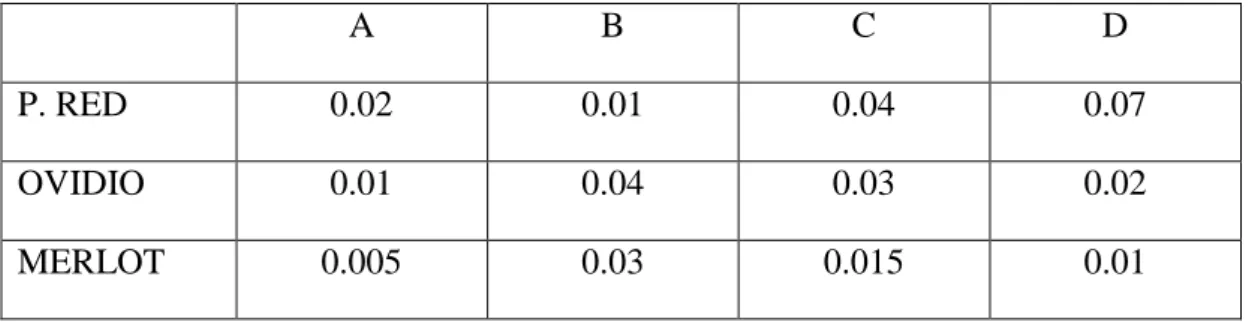
discounts are shown in Table 2 below.
Table 2 – Percentage discounts
A B C D
P. RED 0.02 0.01 0.04 0.07
OVIDIO 0.01 0.04 0.03 0.02
MERLOT 0.005 0.03 0.015 0.01
The problem is to determine how many boxes of each product to be transported from the
source to each destination on a monthly basis in order to minimize the total transportation
cost.
Table 3 - Forming the transportation tableau
A B C D SUPPLY
P. RED 15 10 4 20 15
OVIDIO 7 6 8 3 25
MERLOT 1 9 5 3 10
To form transportation tableau, let i = product to be shipped; j = destination of each product;
s
i = the capacity of source node i; dj = the demand of destination j; xij= the total capacity from
source i to destination j; C
ij= the per unit cost of transporting commodity from i to destination
j. If we suppose that discount is given on each box transported from i to j then the non linear
transportation problem can be formulated as:
Minimize 15x11 + 10 x12 + 4 x13 + 20 x14
7x21 + 6 x22 + 8 x23 + 3 x24
x31 + 9 x32 + 5 x33 + 3 x34
Subject to
x11 + x12 + x13 + x14 = 15
x21 + x22 + x23 + x24 = 25
x31 + x32 + x33 + x34 = 10
x11 + x21 + x31 = 20
x12 + x22 + x32 = 10
x13 + x23 + x33 = 8
x14 + x24 + x34 = 12
where
C11x11 = 15x11– p11x211 C22x22 = 6x22– p22x222
C12x12 = 10x12– p12x212 C23x23 = 8x23– p23x223
C13x13 = 4x13– p13x213 C24x24 = 3x24– p24x224
C14x14 = 20x14– p14x214 C31x31 = x31– p31x231
C21x21 = 7x21– p21x221 C32x32 = 9x32– p32x232
C33x33 = 5x33– p33x233 C34x34 = 3x34– p34x234
If we allow the discounts on each transported product i from the source to each of the
destinations j as given in Table 2, the cost function become:
C11x11 = 15x11– 0.02x211 C22x22 = 6x22– 0.04x222
C12x12 = 10x12– 0.01x212 C23x23 = 8x23– 0.03x223
C13x13 = 4x13– 0.04x213 C24x24 = 3x24– 0.02x224
C14x14 = 20x14– 0.07x214 C31x31 = x31– 0.005x231
C21x21 = 7x21–0.01x221 C32x32 = 9x32– 0.03x232
C33x33 = 5x33– 0.04x233 C34x34 = 3x34– 0.01x234
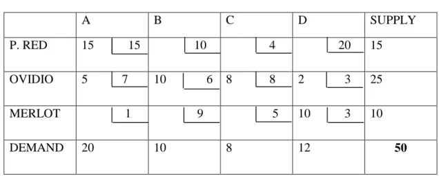
Using the West Corner rule we get the initial basic solution. The solution tableau is as shown
Table 4 – Solution tableau
A B C D SUPPLY
P. RED 15 15 10 4 20 15
OVIDIO 5 7 10 6 8 8 2 3 25
MERLOT 1 9 5 10 3 10
DEMAND 20 10 8 12 50
The initial basic feasible solution is: ̅ = (xB11, x12, x13, x14, xB21, xB22, xB23, x24, x31, x32, x33,
xB34). This from the table is given as ̅ = (15, 0,0, 0, 5, 10, 8, 2, 0, 0, 0, 10) in thousands with
the total transportation cost of Cost = (1,500*15) + (5000*5) + (10,000*6) + (8,000*8) +
(2,000*3) + (10,000*2). Total Cost = GH¢400,000.00.
Now, we use the KKT optimality conditions to improve upon our solution. The partial
derivatives at ̅ for the cost function are given as:
= 14.4
= 10
= 4
= 20
= 6.9
= 5.2
= 7.52
= 2.92
= 1
= 9
= 5
= 1.8
Now we find from the cost equation of the occupied cell;
=
- ui– vj = 0
Thus,
= ui + vj
u1 + v1 = 14.4 u1 + v2 = 10 u2 + v2 = 5.2
u2 + v4 = 2.92 u2 + v1 = 6.9 u2 + v3 = 7.52 u3 + v4 = 1.8
u1 = 0, u2 = -7.5, u3 = -8.62, v1 = 14.4, v2 = 12.7, v3 = 15.02, and v4 = 10.42
We find the net evaluation factor or the reduced costs for the non-basic variables.
=
– u1– v2 = -2.7
=
– u1– v3 = -11.02
=
– u1– v4= 9.58
=
– u3– v1 = -4.78
=
– u3– v2 = 4.92
=
– u3– v3 = -1.4
The presence of negative values for the reduced cost signifies non optimality; hence we
readjust. From the above, the minimum reduced costs for the non-basic variable is x13.
Therefore x13 should enter the basis since it is the most negative reduced cost.
We then move on to next iteration. At the end of this stage of iteration, the basic feasible
solution is ̅ = (15, 0, 0, 0, 5, 10, 8, 2, 0, 0, 0, 10). After adjusting the values x23 entered the
solution. Next we find the cost equation for the occupy cell.
=
- ui– vj = 0
Thus,
= ui + vj
u1 + v1 = 14.4 u1 + v3 = 4 u2 + v1 = 6.9
u2 + v2 = 5.2 u2 + v4= 2.92 u3 + v4 = 1.8
Letting u1 = 0, from the equations we have;
u1 = 0, u2 = -7.5, u3 = -8.62, v1 = 14.4, v2 = 12.7, v3 = 4, and v4 = 10.42
The net evaluation factor or the reduced costs for the non-basic variables is;
=
– u1– v2 = -2.7
=
=
– u1– v4= 9.58
=
– u3– v1 = -4.78
=
– u3– v2 = 4.92
=
– u3– v3 = 9.62
The presence of negative values for the reduced cost signifies non optimality; hence we
readjust. From the above, the minimum reduced costs for the non-basic variable is x31.
Therefore x31 should enter the basis since it is the most negative reduced cost.
We then move on to next iteration. At the end of this stage of iteration, the basic feasible
solution is ̅ = (7, 0, 8, 0, 13, 10, 0, 2, 0, 0, 0, 10). Next we find the cost equation for the
occupy cell.
=
- ui– vj = 0
Thus,
= ui + vj
u1 + v1 = 14.4 u1 + v3 = 4 u2 + v1 = 6.9
u2 + v2 = 5.2 u2 + v4= 2.92 u3 + v4 = 1.8
Letting u1 = 0, from the equations we have;
u1 = 0, u2 = -7.5, u3 = -8.62, v1 = 14.4, v2 = 12.7, v3 = 4, and v4 = 10.42
The net evaluation factor or the reduced costs for the non-basic variables is;
=
– u1– v2 = -2.7
=
– u2– v3 = 11.02
=
– u1– v4= 9.58
=
– u3– v1 = -4.78
=
– u3– v2 = 4.92
=
– u3– v3 = 9.62
The presence of negative values for the reduced cost signifies non optimality; hence we
readjust. From the above, the minimum reduced costs for the non-basic variable is x31.
Therefore x31 should enter the basis since it is the most negative reduced cost. We then move
on to next iteration. At the end of this stage of iteration, the basic feasible solution is
=
- ui– vj = 0
Thus,
= ui + vj
u1 + v1 = 14.4 u1 + v3 = 4 u2 + v1 = 6.9
u2 + v2 = 5.2 u2 + v4= 2.92 u3 + v1 = 1
Letting u1 = 0, from the equations we have:
u1 = 0, u2 = -7.5, u3 = -13.4, v1 = 14.4, v2 = 12.7, v3 = 4, and v4 = 10.42
The net evaluation factor or the reduced costs for the non-basic variables is;
=
– u1– v2 = -2.7
=
– u2– v3 = 28.42
=
– u3– v4 = 4.78
=
– u3– v2 = 9.7
=
– u3– v3 = 14.4
The presence of negative values for the reduced cost signifies non optimality; hence we
readjust. From the above, the minimum reduced costs for the non-basic variable is x12.
Therefore x12 should enter the basis since it is the most negative reduced cost. We then move
on to next iteration. At the end of this stage of iteration, the basic feasible solution is
̅ = (0, 7, 8, 0, 10, 3, 0, 12, 10, 0, 0, 0). Next we find the cost equation for the occupy cell.
=
- ui– vj = 0
Thus,
= ui + vj
u1 + v2 = 10 u1 + v3 = 4 u2 + v1 = 6.9
u2 + v2 = 5.2 u2 + v4= 2.92 u3 + v1 = 1
Letting u1 = 0, from the equations we have;
u1 = 0, u2 = -4.8, u3 = -10.7, v1 = 11.7, v2 = 10, v3 = 4, and v4 = 7.09
=
– u1– v1 = 2.7
=
– u1– v4 = 12.91
=
– u2– v3 = 8.32
=
– u3– v4 = 2.5
=
– u3– v2 = 9.7
=
– u3– v3 = 11.7
Since all the reduced costs for the non-basic variables are all positive, it implies ̅ is the
KKT optimality point. Because optimal solution is our goal, we then proceed to make our
allocation and calculate our total optimal cost of transportation.
From our feasible solution, 7000 boxes of P.Red should be supplied to market zone B, 8000
boxes to market zone C, 10000 boxes of Ovidio to market zone A, 3000 to market zone B,
12000 to market zone D, and 10000 boxes of Merlot be supplied to market zone A. Total Cost
= (10*7) + (8*4) + (10*7) + (3*6)+ (12*3)+ (10*1) thousand. Total Cost = GH¢236,000.
Conclusion
We have described the transportation problem of a company as a non-linear transportation
problem. We applied KKT optimality algorithm to solve the company’s problem. Our
research focused on the model of the non-linear transportation problem for a particular
company in Ghana. It can however be applied to any situation that can be modelled as such.
This paper aimed at solving transportation problem with volume discount on quantity of
goods shipped which is a non-linear transportation problem. Using KKT optimality algorithm,
with a data from a Ghanaian company, it was observed that the optimal solution that gave
minimum achievable cost of supply was the supply of 7000 boxes of P. Red to market zone B,
8000 boxes to market zone C, 10000 boxes of Ovidio to market zone A, 3000 to market zone
B, 12000 to market zone D, and 10000 boxes of Merlot be supplied to market zone A at a cost
of GH¢236,000.
Using the more scientific transportation problem model for the company’s transportation
problem gave a better result. Management may benefit from the proposed approach for their
transportation problem purposes. We therefore recommend that the transportation problem
Our study is limited to a nonlinear transportation problem with concave shape which is as a
result of discount given on volume of goods transported. Unlike the linear transportation
problems, maximization of profit is realized with discounts on large volumes, which means
the determination of the best transportation route that would lead to low transportation cost
and the effective transportation of these goods.
References
Balachandran, V. and Perry, A. (2006) Transportation type problems with quantity discounts. Naval
Research Logistics Quarterly, vol. 23, n. 2, pp. 195–209.
Crama, Y., Pascual J, R. and Torres, A. (2004) Optimal procurement decisions in the presence of total quantity discounts and alternative product recipes. European Journal of Operations Research, vol. 159, n. 2, pp. 364-378.
Goossens, D. R., Maas, A. J. T., Spieksman, F. C. R. and de Klundert, J. J. (2007) Exact algorithms for procurement problems under a total quantity discount structure. European Journal of
Operational Research, vol. 178, n. 2, pp. 603–626.
Hitchcock, F. L. (1941) The distribution of a product from several sources to numerous localities. Journal of Mathematical and Physics, vol. 20, pp. 224-230.
Ojha, A., Das, B, Mondal, S. and Maiti, M. (2010) A solid transportation problem for an item with fixed charge, vechicle cost and price discounted varying charge using genetic algorithm. Applied Soft Computing, vol. 10, n. 1, pp. 100-110.
Sun, M. (1998) A tabu search heuristic problem for solving the transportation problem with exclusionary side constraints. Journal of Heuristics, vol. 3, pp. 205-326.