A Constructive hybrid genetic algorithm for the flowshop scheduling problem

Manuscript received September 5, 2008. Manuscript revised September 20, 2008.

A Constructive Hybrid Genetic Algorithm for the Flowshop

Scheduling Problem

José Lassance de Castro Silva

and Nei Yoshihiro Soma

,

1

Department of Applied Mathematics, Federal University of Ceará, Brazil

2

Department of Computer and Eletronic Engineering, Technologic Institute of Aeronautic, Brazil

Summary

This paper introduces a technique for solving the flowshop scheduling problem. The major idea is to partition the set of feasible solutions into regions in order to diversify the search that is used on a Genetic Algorithm variation. The population is formed by every distinct subject and it is carried out constructively in such a way that any iteration guarantees a diversification on the search for a feasible solution. The problem is a very well known NP-Hard problem and it imposes great challenges for determining its optimal solution in the practice. Computational experiments are reported for the literature instances and the obtained results are compared with other techniques.

Key words:

Scheduling Problem, Genetic Algorithm, Permutations.

1. Introduction

The Flowshop Scheduling Problem (FSP) is defined as given a set of n jobs, J1, J2, …, Jn, to be processed by m

machines M1, M2, ..., Mm. Each job demands m operations

and every job has to obey the same operation flow, i.e. job Jk for k =1,2,..., n is processed first in machine M1, then in

machine M2 and so forth up to Mm. If job Jk does not use

all the machines its processing flow continues to be the same but with time zero whenever that happens. A machine processes just a single job and once it is started it cannot be interrupted up to its completion. It is worth of mentioning that the total search space of possible sequences to be considered is very large and it is bounded by above by O(n!). A solution to the problem consists in processing all the n jobs in the least possible time.

The FSP input is given by a matrix P with m x n non-negative elements, where Pik is associated with job Jk

processing time and machine Mi. Following the four

parameters A/B/C/D [1] notation, the problem is classified as n/m/P/Fmax. The problem is F/prmu/Cmax within [2],

suggested a classification α/β/γ. The FSP is also known to be NP-Complete in the strong sense for m ≥ 3 ([3]). However, for m = 2 it can be exactly solved in polynomial time.

In [4] there is an extensive literature survey – for the last five decades – to the problem and the authors indicate the existence of more than 1,200 Operations Research papers on it, also containing a large diversity of aspects and applications.

In the practice, the exact solution methods for the problem are still limited to small instances, n ≤ 20 and even to them the running time continues to be large. Ruiz et al. [5] summarize practical methods for solving the problem, not necessarily exact ones. The following heuristics that are cited in [5]: PAL ([6]), CDS ([7]); and the Simulated Annealing (SA) metaheuristics cited in [8], , since they will be form the comparison bases of the methodology suggested here.

The FSP algorithmic approach introduced here is a new Genetic Algorithm (GA). It is based on practical observations that indicate that in some problems that rely on permutation of data diversification can supersede intensification. Moreover, under this hypothesis solutions evaluated by the technique are built up in such a way that repetitions are avoided and this is not always the case for the traditional genetic algorithm, since it has a random function that cannot give such a premise. This new method is called HCGA (Hybrid Constructive Genetic Algorithm) and it follows, therefore, all the usual steps of GA one, with the additions mentioned.

Section 2 the FSP is formally stated as a Permutation Combinatorial Optimization problem and the major ideas of HCGA are also introduced. Section 3 presents the computational experiments, while in Section 4 some conclusions are established.

2. The Genetic Algorithm

the problem needs to determine an instance s that minimizes g. A neighborhood N(s) is defined as a solution that can be reached by a single place exchange, also called as a move or movement, of aj and ak, where j, k ∈ {1, …,

n} and j ≠ k. For instance, for n = 3 and s = {a1, a2, a3} a

movement can be s’ = {a1, a3, a2}; s has s’ as a neighbor.

Silva and Soma ([9]) suggested a technique to solve COP denoted by Permutation Heuristic (PH) and it induces diversification among the set of feasible solutions. The idea consists on partitioning S in n neighborhoods N(si). The permutation si that generates N(si) has element i

in the first position and also to every other permutation s ∈ N(si). The total quantity of permutations to any given

neighborhood is set to 2(n-1)(n-2)+4 and this implies in 2n(n-1)(n-2)+4n generated permutations for the problem.

The FSP can also be stated as a COP in the format P = (S, g, n) with the following:

a) An element s = {J1, J2, ..., Jn} from the set of feasible

solutions S represents a permutation of the n jobs. Moreover, it also gives the order in which the jobs have to be processed.

b) Procedure GenEstimate given next determines the total time to be spent to process sequence s. This evaluation is crucial since the overall computational requirements is directly associated with that generation.

I nput : m , n, s, m at rices T( m x n) and P( m x n) . Out put : t g ( t im e necessary t o process all t he n j obs by using sequence s)

/ / Com m ent : m at r ix T has only zeroes init ially . for ( j = 1; j < = n; j + + ) {

for ( i= 1; i< = m ; i+ + ) { if ( i= = 1) {

if ( j > = 2) T[ 1] [ s[ j ] ] = T[ 1] [ s[ j - 1] ] + P[ 1] [ s[ j - 1] ] ; } else {

if ( j = = 1)

{ T[ i] [ s[ 1] ] = T[ i- 1] [ s[ 1] ] + P[ i- 1] [ s[ 1] ] ; } else {

x = T[ i] [ s[ j - 1] ] + P[ i] [ s[ j - 1] ] ; y = T[ i- 1] [ s[ j - 1] ] + P[ i- 1] [ s[ j - 1] ] ; if ( x > = y) T[ i] [ s[ j ] ] = x ; else T[ i] [ s[ j ] ] = y ; }

} } }

t g= T[ m ] [ s[ n] ] + P[ m ] [ s[ n] ] ;

The HCGA follows the major steps of the usual Holland ([10]) Genetic Algorithms framework. In this way, it has initially a set of subjects (initial set of a problem), performs an evaluation for each one (determination of the objective function value), chooses the most well fitted, selects the best ones accordingly with a given metrics and by crossover and mutation (movements) generates new individuals.

The initial and the following populations of HCGA are generated by N(si), from PH given above, and they aim

good solutions from the diversification within S. In addition, HCGA uses the well known 3-Opt Lin and Kernighan [11] heuristic as the mutation operator, since it alters the order in which the jobs are processed and eventually there is intensification in the search.

Since PH is a constructive method and 3-Opt is an intensive local search method, the two types of search are contemplated by HCGA. It is important to note that the choice for those constructive and intensive features stems for the avoidance of a premature and non-optimal convergence of the algorithm. Accordingly with observations in [12], HCGA is defined as [YY]2_nvrY[YNgr]. More details on the theory and evolution of the AG approach are given among others in [13], [14], [15], [16], [17], [18], [19], and [20].

The procedures used in the HCGA for the FSP are: i. A chromosome (an individual of the population)

is defined as a permutation of the n jobs. Every job consist a chromosome gene.The order (from left to the right) in which the jobs appear in it determine their processing order;

ii. The individuals of the population are all evaluated by the same procedure GenEstimate stated before;

iii. A HCGA population has a fixed size of 52 individuals, divided in four groups with 13 individuals each. The algorithm uses a different population every iteration and in total n of them, P1, P2, …, Pn will be considered. An individual of

population Pj, with 1≤j≤n has job j as its first

chromosome element;

iv. Let Pj1, Pj2, Pj3 and Pj4 be the four groups of

population j. The size of 52 was determined experimentally. It was observed that to values lower than 52 the solutions quality were not good enough and to higher values there was no further significant improvements from the increase in the population;

v. The reproduction occurs via the crossover for each individual from group Pj1 with those of Pj2

and the same for Pj3 with Pj4.

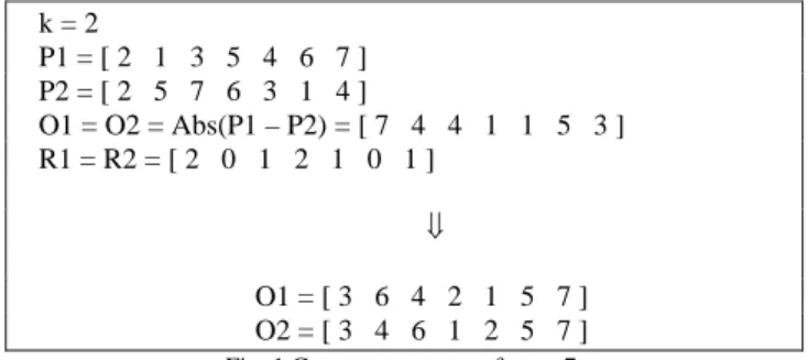
The crossover operator was derived with the idea of generating individuals that do not belong to their parents’ population. To obtain such a feature, admit that P1 and P2 are vectors with n elements each. Their absolute differences are stored in O1=O2=| P1 – P2| and those zero values are set to n. Two auxiliary vectors R1 and R2 with n components are created where R1j and R2j 1 ≤ j ≤ n

indicate the quantity that job j appear in O1 and O2 respectively. If R1j ≥ 2 the first job j found in O1 is

replaced by the first job i of R1, such that R1i = 0, 1≤ i ≤ n.

This implies that R1i = 1 and R1j = R1j-1. The same

Finally, item k+1 will be in the first position both in O1 and O2, where k is the population index that individuals P1 and P2 belong. With this exchange procedure that is quite evolving to describe but very easy to implement in a computer program, there is a guarantee that the resulting individuals’ generated chromosomes will differ from their ancestors. Two additional individuals are generated by doing O1’(j)=O2’(j)=|P1(j)+P2(j)–n| with the same procedure. An example of the suggested crossover operator is given by Figure 1 with n = 7.

k = 2

P1 = [ 2 1 3 5 4 6 7 ] P2 = [ 2 5 7 6 3 1 4 ]

O1 = O2 = Abs(P1 – P2) = [ 7 4 4 1 1 5 3 ] R1 = R2 = [ 2 0 1 2 1 0 1 ]

⇓

O1 = [ 3 6 4 2 1 5 7 ] O2 = [ 3 4 6 1 2 5 7 ]

Fig. 1 Crossover operator for n =7.

After the generation of all crossover of a given population the best fitted individual’s chromosome is selected, i.e. the one with the least objective function value. To modify the order in which the genes (jobs) appear in that chromosome the 3-Opt heuristic is used. This procedure configures the mutation operator of HCGA.

The algorithm stopping criteria for the evolution process and therefore the search occurs only when all the n populations and their respective crossovers have been considered.

Notice that HCGA has many features of a usual Genetic Algorithm but it also has other ones that distinguish it from them. The following steps do not have parallels in GA:

• The population is not randomly generated in order to avoid individual repetitions. Every iteration also is different from their predecessors;

• The crossover operator does not rely exclusively on the preservation of their predecessors’ characteristics. The assumption for this is such that the diversification tries to mimic some the results obtained by practical genetic experiments, such as [21], [22], [23], [24], [25], and [26]. In those experiments the authors deduced that individuals with perfect genetic characteristics did not appear from a mutation process but after a large number of crossovers (diversification). According to these practical approaches mutation has a very high operational cost to be effectively realized and being this not the case for crossovers.

After the implementation and major ideas presentation, it is of vital importance to determine the

algorithm complexity. To find the running time, notice that if η is the number of generations, μ the population size, n the quantity of genes of any chromosome (problem input) and as it is immediate to infer that O(n3) represents the mutation operator complexity, the overall time complexity of HCGA is bounded in the worst case by O(η.μ.n.O(n3)) = O(n4). To specific case, recall that μ is set to 52 while η = 2×2×13×13 = 676. Additionally, the total quantity of solutions to be evaluated by HCGA is (η + μ + 1)n = 729 n = O(n) for any problem.

3. Computational Experiments

The computational experiments carried out to observe the performance of HCGA were executed in a PC-Asus with a clock of 1,8 GHz and 256 Mbytes of RAM and the source program is in ANSI C. Table 1 and 2 presents the mean deviation and CPU time of algorithms HCGA, PAL, CDS, SA, respectively. The 90 problem instances were stated as in Taillard [27] and were obtained in OR-Library [28]. Parameters m and n are also used to divide the experiments in classes. The mean deviation is given by 100×(z – z*)/z*, z is the value determined by a heuristic and z* is the value of the optimal solution. The quantity of problems for each class is 10. HCGA, PAL and CDS had a standard termination while SA could not obtain a solution in some cases. The last three lines of the table give the mean, the miniminum and the maximum values of the standard deviation and CPU time (seconds).

Some observations can be deduced from the experiments (Table 1 and 2):

a) HCGA has the best mean deviation amidst the four methods evaluated, i.e. 8.82% and SA the worst one with 15.50%;

b) PAL had the minimum deviation, 0.70%, for a problem of class (100 x 5). CDS and HCGA had 5.17% and 2.23% respectively;

c) The best deviation performance to HCGA was in class (20 x 5) with 1.77% while to PAL and CDS the values were respectively 5.89% and 4.87%; d) Problems of class (50 x 20) generated the worst

performance for all methods;

Table1: The mean deviation for HCGA, SA, PAL and CDS Class Mean Deviation (%)

(n x m) HCGA SA PAL CDS

1 (20 x 5) 6.71 9.40 10.82 9.49 2 (20 x 10) 10.64 18.60 15.28 12.13 3 (20 x 20) 8.19 32.60 16.34 9.64 4 (50 x 5) 4.79 3.00 5.34 6.10 5 (50 x 10) 12.39 17.00 14.03 12.98 6 (50 x 20) 18.05 28.00 17.94 15.77 7 (100 x 5) 3.77 4.00 2.51 5.13 8 (100 x 10) 4.53 11.00 9.13 9.15 9 (100 x 20) 10.32 15.00 15.55 14.19 Mean 8.82 15.40 11.88 10.51 Minimum 1.77 3.00 0.70 1.80 Maximum 20.86 36.00 24.75 18.42

Table2: The mean running time for HCGA, SA, PAL and CDS Class Time (CPU in seconds) (n x m) HCGA SA* PAL CDS 1 (20 x 5) 0.2 390.0 0.0 0.0 2 (20 x 10) 0.3 408.0 0.0 0.0 3 (20 x 20) 0.7 588.0 0.0 0.0 4 (50 x 5) 1.4 2052.0 0.0 0.0 5 (50 x 10) 2.1 2784.0 0.0 0.1 6 (50 x 20) 3.9 3354.0 0.1 0.2 7 (100 x 5) 6.5 8802.0 0.1 0.2 8 (100 x 10) 10.0 11358.0 0.1 0.5 9 (100 x 20) 17.0 13092.0 0.1 0.6 Mean 4.7 4758.7 0.0 0.2 Minimum 0.1 390.0 0.0 0.0 Maximum 19.0 13092.0 0.1 0.6

* _{It was executed originally in a PC 486 with 33 MHz clock.}

4. Conclusion

The suggested heuristic has many different features from a usual Genetic Algorithm such as the increase of the diversification and the diminishing of crossover operations. The reason to such an approach mimics the behavior of some species as mentioned in the literature.

The computational experiments from the standard benchmarks of the area show that HCGA can be competitive if compared to other heuristic and metaheuristic approaches. It was applied successfully to the FSP and it seems reasonable to suppose, at least in a first moment, that it can solve other Permutation Combinatorial Optimization problems. This hypothesis, however, needs further studies on them.

An attempt to improve the HCGA performance would be the use of other greedy heuristics in order to

obtain more focused criteria to activate new mutations, since it seems that the running time still lies within practical acceptable intervals.

Acknowledgments

The authors acknowledge partial financial support from UFC, ITA and CNPq under process number 302176/03-9.

References

[1] R.W. Conway, W.L. Maxwell, L.W. Miller. Theory of

scheduling. Reading, MA: Addison-Wesley; 1967.

[2] R.L. Graham, E.L. Lawler, J.K. Lenstra, A.H.G. R. Kan.

Optimization and approximation in deterministic sequencing and scheduling: a survey. Annals of Discrete

Mathematics, 5:287–326, 1979.

[3] M.R. Garey, D.S. Johnson, R. Sethi. The complexity of

flowshop and jobshop scheduling. Mathematics of

Operations Research, 1(2):117–29, 1976.

[4] J. N.D. Gupta, E. F. Stafford Jr. Flowshop scheduling

research after five decades. European Journal of

Operational Research 169, 699–711, 2006.

[5] R. Ruiz, C. Maroto, J. Alcaraz. Two newrobust genetic

algorithms for the flowshop scheduling problem. The

International Journal the Management Science (Omega), 34 : 461 – 476, 2006.

[6] D.S. Palmer. Sequencing jobs through a multistage process in the minimum total time - a quick method of obtaining a near optimum. Operational Research Quartetly 16: 101-107, 1965.

[7] H.G. Campbell, R.A. Dudek, M.L. Smith. A heuristic algorithm for the n-job, m-machine sequencing problem. Management Science, 16: B630–B637, 1970.

[8] M. B. Daya, M. Al-Fawzan. A tabu search approach for the

flow shop scheduling problem. European Journal of

Operational Research, l09: 88-95, 1998.

[9] J.L.C. Silva, N.Y. Soma. A heristic for Permutation

Combinatorial Optimization Problems. Proceedings of the

XXXIII SBPO (in Portuguese), Campos do Jordão-SP, Brazil, 2001.

[10]J.H. Holland. Adaptation in natural artificial systems. University of Michigan Press, 1975.

[11]S. Lin, B.W. Kernighan. An Effective Heuristic Algorithm

for the Traveling Salesman Problem. Operations Research,

v.21, p.498-516, 1973.

[12]Alain Hertz and Daniel Kobler. A framework for the

description of evolutionary algorithms. European Journal

Operational Research, 126: 1-12, 2000.

[13]C. R. Reeves (Ed.). Modern Heuristic Techniques for

Combinatorial Problems. McGraw-Hill, London, 1995.

[14]C.R. Reeves. A genetic algorithm for flowshop sequencing.

Computers & Ops. Res., (in review), 1992.

[15]D. E. Goldberg. Sizing populations for serial and parallel genetic algorithms. Proceedings of the 3rd _{International} Conference on Genetic Algorithms. Morgan Kaufmann, Los

Altos, CA, 70-79, 1989.

[16]S. Michalewicz. Genetic algorithm + Data structure =

[17]T. Murata, H. Ishibuchi and H. Tanaka. Genetic Algorithms for Flowshop Scheduling Problems. Computers ind. Engng, Vol. 30, No. 4, pp. 1061-1071, 1996.

[18]I. M. Oliver, D. J. Smith and J.R.C. Holland. A study of permutation crossover operators on the travelling salesman problem. Proceedings of the 2nd International Conference on Genetics Algorithms. Lawrence Erlbaum Associates,

Hillsdale-NJ, 224-230, 1987.

[19]L. Davis. Handbook of Genetic Algorithms. Van Nostrand Reinhold, New York, 1991.

[20]D. Whitley, T. Starkweather and D. Shaner. The traveling salesman and sequence scheduling: quality solutions using genetic edge recombination. Handbook of Genetic

Algorithms. Van Nostrand Reinhold, New York, 350-372,

1991.

[21]P.K. Ingvarsson. Restoration of genetic variation lost - the genetic rescue hypothesis. TRENDS in Ecology & Evolution, Vol.16, 2: 62-63, 2001.

[22]D. T. Pham and D. Karaboga. Cross breeding in genetic optimisation and its application to fuzzy logic controller design. Artificial Intelligence in Engineering, 12:15-20, 1997.

[23]A. P. Bentota, D. Senadhira and M. J. Lawrence. Quantitative genetics of rice: The potential of a pair of new plant type crosses. Field Crops Research, 55: 267-273, 1998. [24]A. K Kahi. et al.. Economic evaluation of crossbreeding for

dairy production in a pasture based production system in Kenya. Livestock Production Science, 65: 167-184, 2000. [25]J.F. Hancock. Implications for plant evolutionary ecology.

TRENDS in Plant Science, Vol. 6, 4: 185, 2001.

[26]H. Michels, D. Vanmontfort, E. Dewil and E. Decuypere, E. Genetic variation of prenatal survival in relation to ovulation rate in sheep: A review. Small Ruminant Research, 29: 129-142, 1998.

[27]E. Taillard. Benchmarks for basic scheduling problems. European Journal of Operational Research 64, 278-285, 1993.

[28]J.E. Beasley. OR-Library: Distributing Test Problems by

Eletronic Mail. Journal of the Operations Research Society,

41: 1069-1072, 1990.

José Lassance de Castro Silva is Associate Professor at the Department of Applied Mathematic of the Federal University of Ceará (Brazil). He holds a B.Sc. and M.Sc. degree in Applied Mathematics at the Federal University of Ceará, in 1990 and 1996, respectively. D.Sc. degree in Eletronic and Computer Engineering at the Technologic Institute of Aeronautic, in 2002. His fields of interest are computer graphics, parallel computing, combinatorial optimization and numerical analysis.