doi: 10.1590/0101-7438.2015.035.02.0251
THERMAL PERFORMANCE OF REFRIGERATED VEHICLES IN THE DISTRIBUTION OF PERISHABLE FOOD
Antˆonio G.N. Novaes
1*, Orlando F. Lima Jr
2,
Carolina C. de Carvalho
2and Edson T. Bez
3Received November 27, 2013 / Accepted August 12, 2014
ABSTRACT.The temperature of refrigerated products along the distribution process must be kept within close limits to ensure optimum food safety levels and high product quality. The variation of product temper-ature along the vehicle routing sequence is represented by non-linear functions. The tempertemper-ature variability is also correlated with the time required for the refrigerated unit to recover after cargo unloading, due to the cargo discharging process. The vehicle routing optimization methods employed in traditional cargo distri-bution problems are generally based on the Travelling Salesman Problem with the objective of minimizing travelled distance or time. The thermal quality of routing alternatives is evaluated in this analysis with Pro-cess Capability Indices (PCI). Since temperature does not vary linearly with time, a Simulated Annealing algorithm was developed to get the optimal solution in which the minimum vehicle traveling distance is searched, but respecting the quality level expressed by a required minimum PCI value.
Keywords: cold chain, vehicle routing, perishable cargo distribution, PCI, TTI.
1 INTRODUCTION
Lifestyle changes over the past decades led to increasing consumption of refrigerated and frozen foods, which are easier and quicker to prepare than the traditional types of food. In order to ensure product quality and health safety (Andr´ee et al., 2010; Wegener, 2010; Daelman et al., 2013), the control of temperature throughout the cold chain is necessary. In fact, a number of factors affect the maintenance of quality and the incidence of losses in fresh food products, such as (a) the initial quality of the commodity; (b) the temperature at which the product is held during handling, storage, transport, and distribution; (c) the relative humidity of the postproduction
*Corresponding author.
1Federal University of Santa Catarina, Department of Production Engineering, 88040-900 Florian´opolis, SC, Brazil. E-mail: [email protected]
2Unicamp – University of Campinas, Faculty of Civil Engineering, 13083-852 Campinas, SP, Brazil. E-mails: [email protected]; carolina [email protected]
environment; (d) the use of controlled or modified atmospheres during storage or transit; (e) chemical treatments for the control of decay or physiological disorders; (j) heat treatments for decay control; and (g) packaging and handling systems (Harvey, 1978). But, since temperature largely determines the rate of microbial activity, which is the main cause of spoilage of most fresh food products (Tarantilis & Kiranoudis, 2002; Mendoza et al., 2004; Giannakourou et al., 2005; James & James, 2010; Ellouze & Augustin, 2010; Mai et al., 2011), continuous monitoring of the full time temperature history usually allows for an adequate control of the process along the short and medium distance distribution situations (Giannakourou et al., 2005). The quality of these products might change rapidly because they are submitted to a variety of risks during transport and storage that are responsible for material quality losses (Pereira et al., 2010; Tassou et al., 2012). Metabolic activities generally increase as storing temperatures are elevated (Borch & Arinder, 2002; McMeekin et al., 2008; Havelaar et al., 2010; Mai et al., 2011). On the other hand, short interruptions in the control of the cold chain may lead to quick deterioration of product quality (Garcia, 2008).
Therefore, the required product temperature range should be maintained from production to con-sumption. However, the main difficulties are encountered at the weakest links or interfaces of the cold chain as delivering, loading or unloading operations and temporary storage where products are generally handled in somewhat uncontrolled temperature ambiences. For an adequate control of the cold chain, some practical recommendations have been presented in the literature. Many investigations have been carried out over the past years on the logistics food chain in order to characterize the temperature variation as a function of product properties, ambient conditions, the size and kind of packaging, the presence and thickness of air layer between the product and the package, solar exposure, and the use of insulating pallet covers. These studies show large variations of temperature in practice (Moureh & Derens, 2000).
This paper reports a Time-Temperature Indicators (TTI) analysis of a distribution of refrigerated products along a route containing a number of retail customers with different demand levels. Time-Temperature Indicators (TTI) can effectively be used to monitor the time/temperature im-pacts on product quality, offering a cost-effective way to detect problematic points in the chill chain. TTI are defined as specific elements collected by electronic equipment that show eas-ily measurable, time and temperature dependent changes that cumulatively indicate the thermal history of the product from the point of manufacture to its destination (Giannakourou et al., 2005; Estrada-Flores & Eddy, 2006; Sahin et al., 2007). One simple type of TTI application involves the registration of temperature measurements along a pre-defined time horizon and the subsequent analysis of this historical data to get the corresponding probabilistic temperature distribution, its average and standard deviation, unexpected temperature rises and drops, and other elements which occur along the transport, storage, and distribution processes (Simpson et al., 2012; Pereira et al., 2010; Estrada-Flores & Eddy, 2006). Process Capability Indices (PCI), on the other hand, can additionally be calculated to yield easily computed evaluation coefficients measured with dimensionless functions on TTI parameters and specifications (Chang & Bai, 2001; Chang et al., 2002; Estrada-Flores & Eddy, 2006). This kind of TTI application helps to reveal undesired thermal conditions that may impair the compliance of product quality require-ments along the cold chain.
The paper analyses alternative vehicle routing strategies intended to minimize travel cost, but at same time keeping thermal PCI performance indicators within the required levels. It is shown that the standard TSP (Travelling Salesman Problem) approach, used to solve classical routing problems where vehicle travel distance or time is minimized, usually leads to temperature restric-tion violarestric-tions. Thus, instead of using a heuristic to get the optimized TSP vehicle routing se-quence, such as the largely employed 2-opt and 3-opt improvement methods (Syslo et al., 2006), other routing strategies, apart from the TSP criterion, can be employed (Ferreira & Pureza, 2012; Faraz et al., 2013). In this paper a Simulated Annealing algorithm was specifically developed to optimize the routing problem.
2 THERMAL ASPECTS OF REFRIGERATED TRANSPORT
regulation requires that refrigerated vehicles have a sufficient cooling capacity to offset the heat load infiltrated through the insulated body, plus an extra capacity calculated as a percentage of the heat leakage. For trucks submitted to only one door opening during an eight-hour period, the percentage extra cooling capacity required is 25%. The extra capacity increases to 200%, for trucks that have 31 to 35 door openings per day. The reserve power is also related to the time-based deterioration of both insulation and refrigerating plant, the differences between test-ing and in-service conditions, the heat of respiration while transporttest-ing fresh produce and the extra-cooling capacity necessary to eliminate defrosting heat (Estrada-Flores & Tanner, 2005). In local delivery, which is the focus of this paper, there is also intensifying demand from legis-lation and retailers for lower delivery temperatures, and increased pressure on fleet operators to improve temperature control (James et al., 2006).
Road transport refrigeration equipment is required to operate reliably in much harsher environ-ments than stationary refrigeration equipment. Due to the wide range of operating conditions and constraints imposed by available space and weight, transport refrigeration equipment has lower efficiency levels than stationary systems. The thermal performance of refrigerated vehicles is also dependent of age, since insulation materials deteriorates with time due to the inherent foam characteristics. Recent data show a typical loss of insulation value of between 3% and 5% per year which can lead to considerable rise in the thermal conductivity after a few years. If a 5% yearly ageing is assumed, a vehicle after nine years of operation may show an increase of approximately 50% in energy consumption and CO2emissions (Tassou et al., 2009, 2012).
The effects of door openings are another important concern in refrigerated cargo transport (Estrada-Flores & Eddy, 2006; Pereira et al., 2010). Tso et al. (2002) used a commercial compu-tational fluid dynamics (CFD) program to model the effects of door openings on air temperature within a refrigerated truck. They carried out a series of experiments to study the effect of door openings with unprotected doors, with air curtains and with plastic strip curtains, showing ex-pressive temperature raises during the unprotected operation.
3 THERMAL PERFORMANCE ANALYSIS
Generally, models that address the prediction of heat and mass transfer during transport can be divided into those that consider the environment within the transport unit (usually in regard to the airflow) and those that concentrate on the temperature of the product (James et al., 2006). Some models combine these aspects and deal with the temporal aspects of transportation: fluc-tuating ambient conditions, door openings, product removal/loading, etc. Other models specif-ically address the effects of transportation temperatures on microbial growth and its influence on food safety.
of door openings are an important concern in refrigerated cargo transport (Estrada-Flores & Eddy, 2006; Pereira et al., 2010). Moureh & Derens (2000) employed a CFD model to study temperature rises in pallet loads of frozen food during distribution. They specifically looked at the times during loading, unloading and temporary storage when the pallets would be in an environment above 0◦C.
A number of papers on refrigerated food transport address the time-temperature evaluation along the cold chain process (Gigiel et al., 1998; James & Scholfield, 1998; Tsironi et al., 2001; Smolander et al., 2004; Giannakourou et al., 2005; Estrada-Flores & Eddy, 2006; Pereira et al., 2010; Nga, 2010). The main purpose of maintaining good temperature control during re-frigerated transport is to decrease the rate of microbial growth and hence maintaining the safety and eating quality of the food (Zhou et al., 2010). In fact, there are many microbial models that can be applied to modelling the growth of microorganisms in food during transport. But, according to James et al. (2006), relatively few studies have been published specifically on the refrigerated transport subject. Even fewer of these have looked at the fully integrated approach of combining dynamic microbial growth modelling with heat and mass transfer models that could represent the characteristics of a food distribution system (James et al., 2006). However, in short-distance transportation of refrigerated food products, as in the case of this work, it suffices to observe that the temperature of the product is maintained within pre-established limits. This condition is adopted in a number of studies reported in the literature based on Time-Temperature Indicators (TTI).
Papers investigating the thermal performance of refrigerated vehicles can be classified into four groups: (a) approaches of pure theoretical nature, (b) performance laboratory tests (c) field data gathering, and (d) TTI based simulations. Studies of the first group use pure mathemati-cal CFD models based on physimathemati-cal aspects of heat transfer (Cuesta et al., 1990; Zhang et al., 1994, Campa˜none et al., 2002; Flick et al., 2012; Hoang et al., 2012a,b). In the second group are the papers describing controlled laboratory tests, such as Moureh & Derens (2000), Tso et al. (2002), Estrada-Flores & Eddy (2006), and Garcia (2008). In the third group are the papers involving field tests, with information eventually supplemented with laboratory data, such as the CoolVan experiment (Gigiel et al., 1998; James & Scholfield, 1998; James et al., 2006), as well as other similar efforts (Giannakourou et al., 2005; Pereira et al., 2010; Nga, 2010). The fourth group comprises TTI – Time-Temperature Indicator analyses, usually employing com-puter simulations (CoolVan Manual, 2000, Hoang et al., 2012a,b). Of course, a good part of these papers employ combined methods. In this paper, the approach (d) will be used, involv-ing time-temperature indicators (TTI) associated with simulation of the thermal performance of refrigerated vehicle tours.
presented in this work is essentially intended to be used in the planning phase of the problem, which requires an approximate accuracy level. For further applications to real problems, more accurate data should be sought, and laboratory tests could eventually be contemplated in such situations. Field tests to gather thermal data, on the other hand, would be acceptable in devel-oping countries like Brazil only under rigid technological and experimental control, a condition hard to achieve presently (Pereira et al., 2010). As a result, approach (d) was selected for this application, involving time-temperature indicators (TTI) associated with thermal performance simulation of refrigerated vehicle tours.
A number of papers on refrigerated food address the TTI evaluation along the cold chain process (Gigiel et al., 1998; James & Scholfield, 1998; Jacxsens et al., 2002; Giannakourou & Taoukis, 2003; Giannakourou et al., 2005; Estrada-Flores & Eddy, 2006). The main purpose of maintain-ing good temperature control durmaintain-ing refrigerated transport is to decrease the rate of microbial growth and hence maintaining the safety and eating quality of the product. In fact, there are many microbial models that can be applied to represent the growth of microorganisms in food during transport. But since temperature largely determines the rate of microbial activity, which is the main cause of spoilage of most fresh and frozen food products, continuous monitoring of the full time temperature history usually allows for the adequate control of the process along short and medium distance distribution situations.
One of the most systematic attempts to predict the temperature of refrigerated food during multi-drop deliveries has been the CoolVan research programme. CoolVan is a software developed by the Food Refrigeration and Process Engineering Research Centre at the University of Bristol, UK. The brief description set forth was extracted from Gigiel (1997), Gigiel et al (1998), and from the Cool Van Manual (2000). The objective of CoolVan is to aid the design and operation of small and medium delivery vehicles intended to distribute refrigerated food products (Gigiel, 1997; Gigiel et al., 1998; James & Schofield, 1998; James et al., 2006; CoolVan Manual, 2000). The software contains a mathematical model that predicts food temperatures inside a refrigerated delivery vehicle, analysing the temperature changes that take place during a delivery journey as well as the energy used by the refrigeration equipment. The model is solved using an implicit finite difference method. It starts with the given initial conditions and proceeds to the end of the journey with variable time steps. The time step is increased when there are few events during the journey. However, the time step is reduced and the program slows down in order to model in detail any event which occurs along the route as, for example, when the vehicle stops and the door is opened. In this way the program is able to model the details of the journey accurately, while at the same time, running at the fastest possible speed. It shows the thermal consequences of changes in delivery patterns, the weather, the vehicle construction characteristics, its refrigeration system, and the type and mass of the food transported.
heat ingress directly from outside and from personnel entering to select and remove product. On the other hand, the design of the refrigeration system has to allow for extensive differences in load distribution, dependent on different delivery rounds, days of the week and the removal of product during a delivery run. A refrigeration system’s ability to respond to sudden demands for increased refrigeration is often restricted by the power available from the vehicle. All these problems converge to produce a complex interactive system. With so many interacting variables it is not feasible to obtain, by purely theoretical means, the reasoning required to design and to operate vehicles that would maintain the required food temperatures. Thus, the CoolVan research project was set up to provide a predictive model that would assist in specifying the design of, and the equipment for small and medium delivery vehicles. Operators of the vans need to know in advance whether a particular vehicle, on a particular route, under given ambient conditions, will be able to deliver food at the correct temperature levels (Gigiel et al., 1998).
The CoolVan program is divided into three parts. The first part allows the user to change over a large number of different variables that are input into the main program: the weather, the way the vehicle is used, its construction, the refrigeration plant and the product that is put in it. The second part of the program does the actual calculations and puts these into an output file that can be saved for future reference or viewed in another application. The last part of the program plots the output data graphically on the screen to allow the user to see what is going on during the journey. Vehicle data are fed into the CoolVan program: the thermal properties of the insulation system, the year of the van manufacture, the ageing rate which depends on the vehicle maintenance characteristics, etc. Then, the program calculates the reduced thermal properties of the vehicle insulation. The mathematical structure of the program also allows different external heat transfer coefficients to be entered for each side of the vehicle. Solar radiation onto each surface of the van is modelled separately. The infiltration of outside air into the van is dependent on the van structure, the degree of maintenance and the speed of the vehicle. These effects were measured empirically in several vans, allowing for the fitting of appropriate equations and parameters into the model.
Controlling temperature during Infiltration of air into the vehicle during door openings is also an important issue. Once the door is opened, the amount of air infiltrating the vehicle approximately increases linearly with time (Gigiel et al., 1998). Vertical air curtains, plastic strip curtains, in-ner lightweight sliding doors or shielding are sometimes used on doors in order to limit the air exchange through them. To accurately model the air exchange in a particular van it is necessary to perform empirical measurements. However, real measurements of the air exchange rate on several vans showed that a reasonable approximation is that it varies as a function of the height and width of the door only.
4 PROCESS CAPABILITY INDICES TO ASSESS TTI DATA
4.1 Capability Indices for Normally Distributed Data
Usually, capability indices are employed to relate the process parameters to engineering specifi-cations that may include unilateral or bilateral tolerances, with or without a target value (nominal value). The resulting indices are dimensionless and provide a common, easily understood way for quantifying the performance of a process. In this application, the monitored variable is the temperatureθinside the vehicle along a typical distribution journey of refrigerated food products, with meanµand standard deviationσ. In this case there are two-sided specification limits for
θ, respectively the upper valueU S Land the lower valueL S L. Four capability indices are com-monly used for variables normally distributed: Cp,Cpk,Cpm andCpmk (Gonc¸alez & Werner,
2009). TheCpindex is defined as
Cp=
U S L−L S L
6σ . (1)
Clearly, the aim of process control is to makeCpas large as possible. The adoption of theCp
index presupposes that the variableθis normally distributed and that the meanµis equal to the specified target valueθT. The coefficientCp is defined as the ratio of the allowable tolerance
spread and the actual spread of the data. IfCp > 1, it indicates that the temperature variation
fits within the specified limits. In practice, ifCp < 1, the process does not meet the defined
specifications; if 1 ≤ Cp < 1.33 the process probably meets the requirements but additional
attention must be taken; ifCp ≥1.33 the process is fully capable (Gonc¸alez & Werner, 2009).
The six-sigma coverage represents the spread of 99.73% of the data in normally distributed pro-cesses. On the other hand, the eight-sigma coverage, which represents the case withCp≥1.33,
covers practically 100% of the data in similar circunstances. In practice, there are cases in which the process is not centred on the target valueθT, i.eµ=θT. To avoid such drawback, the index
Cpk is defined
Cpk=min
U S L−µ
3σ ,
µ−L S L 3σ
. (2)
On the other hand, the indexCpm explicitly considers the distance between the mean and the
target valueθT (Gonc¸alez & Werner, 2009):
Cpm =
U S L−L S L
6σ2+(µ−θ T)2
. (3)
For practical purposes, sample estimators can be used for calculating the above indices.
4.2 Capability Indices for Non-Normal Data
population, by using specific factors in computing the deviations above and below the variable mean. The method is based on the idea thatσ can be divided into upper and lower deviations,
σU andσL, which represent the dispersions of the upper and lower sides around the mean µ,
respectively. An asymmetric probability density function f(θ )can be approximated with two normal pdfs (Chen & Ding, 2001)
fU(θ )=
1 2σU
∅
θ−µ
2σU
and fL(θ )=
1 2σL
∅
θ−µ
2σL
, (4)
with the same mean µbut different standard deviations 2σU and 2σL, where∅represents the
standard normal pdf. The upper and lower sides of f(θ )are approximated with the upper side of fU(θ )and the lower side of fL(θ ), respectively. The values ofσU andσL are computed as
(Chang et al., 2002)
σU =Pθσ andσL =(1−Pθ)σ, withPθ = Pr{θ ≤µ}. (5)
The value ofCpis defined as (Chang & Bai, 2001)
Cp = min
U S L−L S L
6×2σU
,U S L−L S L
6×2σL
= min
U S L−L S L
6×2Pθσ
, U S L−L S L
6×2(1−Pθ)σ
(6)
= U S L−L S L 6σ min
1 2Pθ
, 1
2(1−Pθ)
.
MakingDθ =1+ |1−2Pθ|, expression (1) can be simplified to
Cp=
U S L−L S L 6σ
1 Dθ
, (7)
where 1/Dθis a corrective coefficient on (1) due to the skewness of the probability distribution
ofθ. On the other hand, according to Chang et al. (2002), the value ofCpkcorrected for skewness
can be estimated as follows. First, the upper and lower capability indices are defined as
C(pkU) =U S L−µ 3×2σU
=U S L−µ 6Pθσ
, (8)
C(pkL) =µ−L S L 3×2σL =
µ−L S L 6(1−Pθ)σ
. (9)
The PCI of the temperatureθ, for the case of two-side specifications (upper and lower values) is
Cpk =min
C(pkU),C(pkL)=min
U S L−µ
6Pθσ
, µ−L S L
6(1−Pθ)σ
. (10)
In Equations (8) and (9), 2σU and 2σLare used in place ofσ to reflect the degree of skewness in
repeating the value given by (1). However, if it is skewed, the value ofCpk given by (10) is
smaller than the standard one given by (1). The numerical estimation ofCpandCpkis performed
as follows. Let(θ1, θ2, . . . , θn)be the sample containingnvalues of the temperatureθ. The mean
ˆ
θand the standard deviationσˆ of the sample are computed. The probabilityPθ can be estimated
by using the number of observations less than or equal toθˆ(Chang et al., 2002):
ˆ Pθ ∼=
1 n
n
i=1
g(θˆ−θi), (11)
whereg(x)=1 forx ≥0 andg(x)=0 forx<0. ThenCpk can be estimated by substituting
ˆ
µ, σˆ, and Pˆθ forµ, σ and Pθ respectively in Eq. (10). In this application the series of TTI
data are skewed (see Section 6.4), and the method of Chen & Ding (2001) has been employed accordingly to getCpkvalues.
A fourth capability index Cpmk is used when the mean µ departs from the target value θT
(Gonc¸alez & Werner, 2009). In this application there is no target value for the temperatureθ, being only necessary to respect the two-sided specified limits, namelyL S LandU S L. Conse-quently, the indexCpk was adopted.
5 PROBLEM DESCRIPTION
The objective of the analysis is to investigate a regional distribution of ready-to-eat refrigerated meat products (ham, turkey and chicken breasts, salami, sausage). Other studies analysing distri-bution schemes of perishable products are Oswald & Stirn (2008), Yu & Nagurney (2013), and Faraz et al. (2013). The urban distribution district is located about 84 km from the base depot. The served urban district has an approximated area of 73 sq.km, where 12 retail shops are lo-cated, as shown in Figure 1. Traditionally, the optimal sequence of points to be visited is obtained with a TSP (Travelling Salesman Problem) algorithm, that yields the shortest Hamiltonian cy-cle, which includes, in this application, all the retail outlets, plus the depot. Figure 1 depicts the TSP route obtained with a 3-opt local search heuristic (Syslo et al., 2006), with a total extension of 204.1 km.
Figure 1– Distribution of refrigerated food in the district: the TSP vehicle route.
operation (to avoid discharging gases to enter the cargo compartment). This situation is shown in Figure 2 when the truck is travelling from client 10 to client 11, and from client 12 to client 3. Normally, the search for an optimal vehicle routing sequence requires quite a number of com-binatory evaluations. On the other hand, the process of obtaining accurate TTI data is not a simple task since it requires special laboratory settings and/or elaborate field tests. One alterna-tive possibility is to apply the simulation approach, such as the CoolVan software (Section 3), in order to gather basic TTI data to be used in a computer aided routing analysis. This is because the CoolVan program does not permit automatic replications of the runs, whereas combinatorial routeing analysis implies automatic combinatorial changes of the delivering sequences in order to obtain the resultingCpk coefficients and the traveling distances.
This line of research has some points in common with the paper by Oswald & Stirn (2008). Their approach differs from the present investigation in two aspects. First, the variable that expresses product quality in our research is temperature, whereas in Oswald & Stirn paper (2008) product quality (fresh vegetables) is based on market acceptance: one has 100% quality when the product can be sold entirely at the current market price and the quality drops to 0% when the product loses completely its commercial value (Oswald & Stirn, 2008). Second, the mathematical routing model developed by these authors builds up the routes to be assigned to the vehicles step by step, while in this application there is only one truck and the route sequence is defined in a combinatorial way.
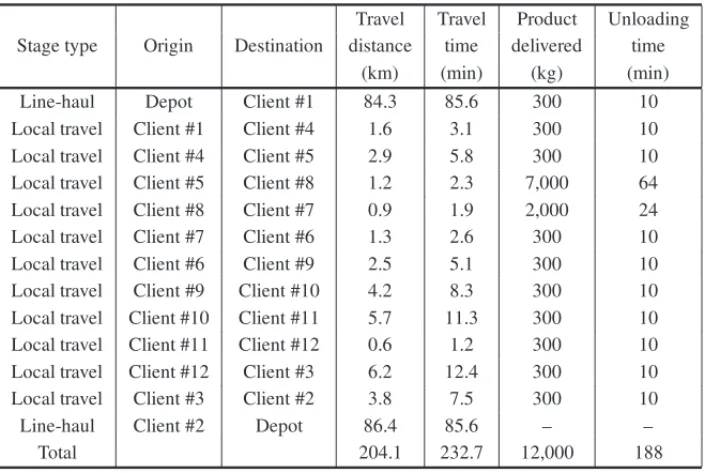
5.1 CoolVan route simulation
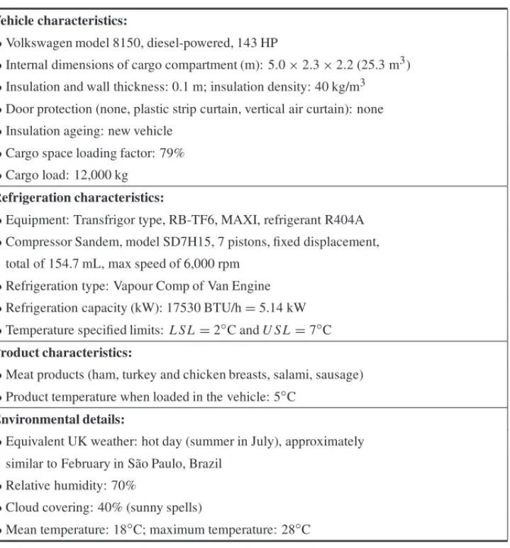
The CoolVan software is still not available commercially but its developers kindly accepted to ran basic routing configurations to serve as a data basis for this application. The necessary in-puts for the CoolVan simulation are presented in Table 1. Next, the data of the food products are fed into the CoolVan program (CoolVan Manual, 2000). The product is ready-to-eat refrigerated meat products (ham, turkey and chicken breasts, salami, sausage). A total of 12,000 kg of as-sorted products are distributed in the daily round, with two retailers receiving larger quantities (7,000 and 2,000 kg respectively), while the other ten clients getting 300 kg each (Table 2). The basic delivery information shown in Table 2, and in Figure 2, illustrates the TSP route. Table 2 also shows the distances travelled along the various segments of the TSP route and the delivering times at the retail premises. It is worth to notice, in Figure 2, the sharp changes of the internal vehicle temperature in the last phases of the simulation process, when the product mass inside the van gets successively smaller.
Table 1– CoolVan simulation inputs.
•Vehicle characteristics:
•Volkswagen model 8150, diesel-powered, 143 HP
•Internal dimensions of cargo compartment (m): 5.0×2.3×2.2 (25.3 m3)
•Insulation and wall thickness: 0.1 m; insulation density: 40 kg/m3
•Door protection (none, plastic strip curtain, vertical air curtain): none
•Insulation ageing: new vehicle
•Cargo space loading factor: 79%
•Cargo load: 12,000 kg
•Refrigeration characteristics:
•Equipment: Transfrigor type, RB-TF6, MAXI, refrigerant R404A
•Compressor Sandem, model SD7H15, 7 pistons, fixed displacement, total of 154.7 mL, max speed of 6,000 rpm
•Refrigeration type: Vapour Comp of Van Engine
•Refrigeration capacity (kW): 17530 BTU/h=5.14 kW
•Temperature specified limits:L S L=2◦C andU S L=7◦C
•Product characteristics:
•Meat products (ham, turkey and chicken breasts, salami, sausage)
•Product temperature when loaded in the vehicle: 5◦C
•Environmental details:
•Equivalent UK weather: hot day (summer in July), approximately similar to February in S˜ao Paulo, Brazil
•Relative humidity: 70%
•Cloud covering: 40% (sunny spells)
•Mean temperature: 18◦C; maximum temperature: 28◦C
The results of the CoolVan simulations are saved in Excel format. Figure 2 exhibits the TTI results obtained with the CoolVan software for the TSP sequence. The simulation starts with the outbound line-haul phase, which goes from the depot to the first client in the district. It is fol-lowed by the delivering visits, intercalating cargo discharging tasks with vehicle travel between successive delivery points. Finally, there is the inbound line-haul segment, linking the last served client to the depot.
5.2 Temperature variation modelling
Table 2– Input data for the TSP sequence of delivery points.
Travel Travel Product Unloading Stage type Origin Destination distance time delivered time
(km) (min) (kg) (min)
Line-haul Depot Client #1 84.3 85.6 300 10 Local travel Client #1 Client #4 1.6 3.1 300 10 Local travel Client #4 Client #5 2.9 5.8 300 10 Local travel Client #5 Client #8 1.2 2.3 7,000 64 Local travel Client #8 Client #7 0.9 1.9 2,000 24 Local travel Client #7 Client #6 1.3 2.6 300 10 Local travel Client #6 Client #9 2.5 5.1 300 10 Local travel Client #9 Client #10 4.2 8.3 300 10 Local travel Client #10 Client #11 5.7 11.3 300 10 Local travel Client #11 Client #12 0.6 1.2 300 10 Local travel Client #12 Client #3 6.2 12.4 300 10 Local travel Client #3 Client #2 3.8 7.5 300 10 Line-haul Client #2 Depot 86.4 85.6 – –
Total 204.1 232.7 12,000 188
in a TTI data sequence (Sahin et al., 2007; Simpson et al., 2011). However, in short-distance distribution cases of refrigerated products, as in the present work, it suffices to register the tem-perature values in order to verify whether they respect the thermal requisites reflected on PCI values (Section 4).
The theoretical basis to analyze the temperature variation of refrigerated products along time is the Newton’s Law of cooling. Suppose that a body, with initial temperatureθ0, is allowed to
cool in a compartment which is maintained at a constant temperatureθ1, withθ1 < θ0. Let the temperature of the body beθat timet. Then, the Newton’s law of cooling is
dθ
dt = −cs(θ −θ1), (12)
withθ=θ0fort =0, and wherecsis a positive proportionality constant. Conversely, ifθ0< θ1,
cs < 0. Suppose a quantity of cargo, with mass m and temperatureθ0, is set inside an empty
refrigerated bin. Departing from the Newton Law of cooling, a simple thermal balance leads to (Alvarez & Flick, 1999; Hoang et al., 2012b)
mC∂θ
∂t =βH(θ−θ1), (13)
whereCis the specific heat capacity of the product (J kg−1K−1),His the heat transfer conduc-tance of the product (W K−1) andβis a constant. The integration of (13) yields an exponential decay function onθ.
from the depot to the first visited retail outlet; (2)product unloadingat retailer premises; (3) vehicle travelfrom one served retail outlet to the next; (4)inbound line-haul, corresponding to the travel from the last served client back to the depot. A general mathematical expression, to represent the internal vehicle temperature variation along the route, was defined to be fitted to CoolVan simulation results
θtB =a0(θtA)a1(θext)a2exp
βH(tB−tA)
mC
, (14)
where
• tA=starting time of the phase under consideration;
• tB =time when the phase under consideration ends;
• θtA andθtB =temperature at timestAandtBrespectively;
• H =heat transfer conductance of the product, (W K−1); • C=thermal capacity of the product (J kg−1k−1);
• m=mass of the product inside the vehicle at the phase under consideration (kg); • a0,a1,a2andβare constants to be fitted.
Since in this case the type of product does not vary along all the CoolVan simulation, the values ofHandChave been calibrated together withβ, and Eq. (14) reduces to
θtB =a0(θtA)a1(θext)a2exp
β(tB−tA)
m
, (15)
The fitting of constants in Eq. (15) was based on CoolVan simulation values obtained for one vehicle type only, the one described in Table 1. Thus, these results should be understood as preliminary, and should not be extended to other situations. New CoolVan runs are under way, considering other vehicles and other visiting patterns. In the adjusted equations, the mass of the product inside the vehicle in expression (15) is expressed as a fraction of the total vehicle capacity. Furthermore, in the delivery runs analysed in this application, the vehicle leaves the depot with a 100% load, and returns empty to the depot.
a) Outbound line-haul phase (line-haul I):Since the vehicle leaves the depot with a 100% load,m = 1 in Eq. (15). For this phase, considering the vehicle carries the same full cargo load(m=1)and the external ambient temperature was not statistically significant, Eq. (15) reduces to
θtB =θtAexp[β(tB−tA)]. (16)
Two vehicle displacement intervals were considered: (a) 0 ≤ T ≤ 20 sec, leading to
β = −0.7670, and (b) T > 20 sec, leading to β = −0.0044. In addition, a lower limit of 4◦C for the temperatureθj was imposed for this phase (meaning the refrigeration
b) Cargo unloading phase: a0=0.3234;a1=1;a2=0.4517;β =0.00081 in relation (15).
The product mass varies during the unloading process. AssumingtB−tAis the duration
of the unloading phase,mAis the mass at the beginning of the cargo unloading phase, and
mB is the mass at its end, one interpolates linearly over time to determine the value of
m. The regression analysis led toR2 = 0.965, and the adjusted constants have shownt Student values significant at a 0.05 level.
c) Vehicle local travel phase: a0=1.4172,a1=0.5869;a2=0.0845 andβ = −0.0007 in
relation (15). Heremis constant and evaluated at timetA. The regression analysis led to
R2=0.913, and the adjusted constants showedtStudent values significant at a 0.05 level.
d) Inbound line-haul phase (line haul II):the expression to compute the temperature variation for the inbound line-haul is similar to the outbound line-haul phase. In this phase, the initial temperature is equal to the vehicle air temperature at the moment the last cargo delivery is accomplished. The temperature drops toθ1=4◦C after an approximately elapsed time of 2 minutes. It is also assumed that no chilled product is sent back to the depot, only working elements such as racks, fittings, empty trays, etc., remain in the truck. An equivalent mass equal to 2.5% of the total load was assumed for such elements, and thus m = 0.025. Applying Eq. (16) for this time interval, one getsβ = −0.0112. ForT ≥2 min to the end of the journey, the temperature remains constant and equal to 4◦C.
5.3 TTI generating module
For a specific routing sequence, the TTI model developed on CoolVan data estimates the travel time between successive delivering stops, the unloading times at different retailer premises, and the line-haul times. Table 2 is an example corresponding to the TSP route. A TTI time series is then constructed assuming one-minute intervals, in which each element is associated with the corresponding phase in the routing process. In the sequel, the vehicle internal temperature is estimated with the equation, indicated in Section 5.2, that corresponds to the phase in which the distribution process is at the moment. An element of the TTI data series is composed by the following elements: (a) element number, (b) phase type, as defined in Section 5.2, (c) starting timet0(min) of the event, (d) termination timet1(min) of the event, (e) temperature θ1 (◦C)
at timet1, estimated with the appropriate equation, (f) last served client number if phase type
is local travel, and zero otherwise, (g) next visiting client if phase type is local travel, or the servicing retailer number if it is an unloading phase. Along the computation stages one has
θ0(j) =θ1(j−1) for j =1,2, . . .andθ1(0) = θini, whereθini is the cargo temperature when it is
loaded in the vehicle at the depot.
Figure 3– Histogram of the internal vehicle temperature for the TSP routing alternative.
6 SIMULATED ANNEALING ALGORITHM TO OPTIMIZE
THE ROUTING SEQUENCE 6.1 Simulated Annealing
The subject of combinatorial optimization is the development of efficient techniques to find minimum or maximum values of a function with many integer (or binary) variables. Such a function, generally called the objective or cost function, represents a quantitative measure of the performance quality or goodness of a system. Exact methods are computationally unpractical for larger problems with many integer or binary variables and restrictions. In such cases heuris-tics are usually employed. One basic strategy to solve combinatorial problems is the iterative improvement method. In iterative improvement, one starts with the system in a known configu-ration, or with an initial solution chosen randomly. A standard rearrangement process is applied to all components of the system until a rearranged configuration, which improves the cost func-tion, is found. The rearranged configuration is now assumed as the new configurafunc-tion, and the process continues until no further improvements can be found. Iterative improvement comprises a search in the space of feasible solutions for rearrangement steps that will lead downwards to-ward the global minimum. But this searching process may get stuck in a local minimum. Thus, it is necessary to carry out the process many times, starting from different random configurations and choosing the best solution, which will be taken as the optimum.
gener-ally applicable meta-heuristic for solving combinatorial optimization problems. The algorithm is based on a combination of ideas from two different fields: statistical physics and combinatorial optimization. On the one hand, it can be viewed as an algorithm simulating the physical anneal-ing process of solids to their minimum energy states. On the other hand, it can be considered as a generalization of local search algorithms, which play an important role in combinatorial optimization.
The simulated annealing algorithm starts off with a given initial solution, very often chosen at random, and continuously tries to move from a current solution to one of its neighbours by ap-plying a generation mechanism and an acceptance criterion. The acceptance criterion allows for sporadic deteriorations in the cost function in a limited way. This is controlled by a parameter that plays a similar role as the temperature in the physical annealing process. The possibility of deteriorations makes the SA algorithm more general than pure iterative improvement algo-rithms, in which only strict improvements are applied. The resulting effect is that the annealing algorithm can systematically avoid local minima in order to arrive at a global minimum (Aarts & Korst, 1989).
Metropolis et al. (1953) developed a simple algorithm that can be used to provide an efficient simulation of a collection of atoms in equilibrium at a given temperature. Using a cost func-tion in place of energy, and defining configurafunc-tions by a set of parameters{xi}, Hastings (1970)
generalized the Metropolis procedure to treat iterative improvement optimization problems out-side statistical physics, and solving them in an analogous way. Now, temperature is simply a control parameter expressed in the same units as the cost function. In our application, in order to avoid duplication of terms, we call itGT – generalized temperature. The annealing process, as implemented in the Metropolis/Hasting procedure, differs from iterative improvement tech-niques in that the former avoids getting stuck in local minima, since transitions out of a local optimum are always possible at intermediate temperatures. In general terms, the SA method to solve optimization problems follows the computing sequence depicted in Figure 4.
A number of scientific articles have been published on SA applications to the solution of en-gineering problems (Correia et al., 2000; Jimenez et al., 2002; Lin et al., 2009). Specifically applications on vehicle routing problems, which is the main focus of this article: Aarts, 1989; Breedam, 1995; Osman, 1998; Mauri & Lorena, 2006; Leung et al., 2013; Hamzadayi et al., 2013.
6.2 Simulated Annealing applied to the distribution of refrigerated food
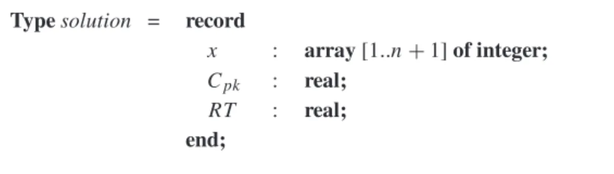
Let us initially define a data “type” in pseudo-code: Typesolution = record
x : array[1..n+1]of integer; Cpk : real;
RT : real;
end;
1 The system under analysis has a representative state described by ann-dimensional vectorx, for which the function to be minimized isf(x).
2 Letibe the step counter of the number of Monte Carlo iterations; 3 The function must return a scalar quantity.
4 The generalized temperatureG Tis a scalar quantity with the same dimension as f(x).
5 Initial step,i=1: Select an initial configurationxB(Bmeansbefore);
6 Set the initial generalized temperature to a high valueG T0; 7 Calculate the function value before the transition: fB= f(xB);
8 Choose a transitionxat random;
9 Do the trial transition asxA=xB+x(Ameansafter);
10 Calculate the function value after the transition fA= f(xA);
11 Computef = fA− fB:
(a) Iff ≤0, accept the new statexAand makexB=xA;
(b) Iff >0:
(I) Generate a random numberrsuch that 0≤r≤1; (II) Accept the statexAonly ifr<exp
−G Tf; 12 If the statexAis accepted, makexB=xA;
13 Reduce the temperatureG Tby some small value:G T−ǫG T←G T
14 Increase the Monte Carlo step by one:i←i+1; 15 IfG T>G Tmingo to 8, otherwisex=xBand End;
Figure 4– General SA computing structure.
The data-type contains, first, the mentioned array representing the ordering position of the clients, plus the depot. Next it appears the variableCpk, which is the correspondingPC I value computed
for the vector x representing the visiting sequence. Finally, RT is the total route extension, starting from the depot and terminating back to it when all delivering tasks are accomplished. Two variables of typesolutionare defined: ∅band∅a, the first one representing the candidate
solution obtained before the SA improvement routine is applied and, the second, the candidate solution generated afterwards.
In the application, two exploratory stages, indicated byk, are considered. In stagek=1 a candi-date solution, represented by the vectorx, is defined by a Monte Carlo routine, with the position of each client in the visiting sequence fully generated at random. This is done to allow the SA procedure to explore prospective solutions covering all the set of possibilities, thus avoiding local minima. The sub-optimal solution obtained at the end of stage 1, represented by variable∅b,
will serve as the initial candidate solution for stage 2.
selected at random in∅b.x. The positions of these two clients are exchanged mutually in order
to generate variable∅a.x, with the remaining clients keeping the same positions they occupied
before in candidate solution∅b. With this approach the SA improvement sequence will explore
closer neighbouring possibilities, thus avoiding too large jumps over the overall set of solutions. Figure 5 shows the pseudo-code of procedurevehicle route(k), that performs the generation of a vehicle route according to the stagekof the SA routine. Other intermediate formulations can also be adopted. For example, one could select a clientxiat random in∅b.x, and maintain fixed
in∅a.x all the positions of the clients located to the left of xi in∅b.x. Next, one shuffles at
random all the clients located at the right side ofxi in∅b.x, and then putting the result in∅a.x.
This scheme brings an intermediate degree of randomness between the other two alternatives. For this application, however, this latter scheme was not necessary because the mathematical structure of the problem led to a rapid SA convergence, as will be explained later.
In applying the SA heuristic to this problem, it is necessary to define the initial value for the generalized temperature (GT0). Investigating the maximum possible route extension for the problem analised in this work, one can see that 300 km is a likely value. With an adequate margin, it was setGT0=500 km. At each step of the SA meta-heuristic, the generalized temperature is
decreased according to a cooling ratert =0.99. This selected slow value temperature decreasing rate of 1% allows for a gentle downward trajectory, thus emulating the statistical mechanics annealing process. On the other hand, a minimum generalized temperature levelGTmin =0.01
(practically zero) was adopted.
The initialization part of the SA procedure starts with the definition of an initial vectorxB
gen-erated by a Monte Carlo routine, as explained before. WithxBand the distance matrix available
for this application, the total route extension RTB is computed. Similarly, entering the
proce-dure to compute process capability indices (PCI), the corresponding value ofC(pkB)is determined (Section 4). The triad{xB,C(B)
pk ,RTB}will constitute variable∅b.
Let us define a temporary optimum valueL∗for the route extension that is changed whenever a smaller value of RT is encountered. In the initialization process, ifC(pkB) < 1.33 (meaning the candidate solution is not acceptable), the valueL∗=GT0is adopted. Otherwise, ifC(pkB) ≥1.33,
L∗ =RTB is assumed. Next, the computer program enters the SA routine proper. The
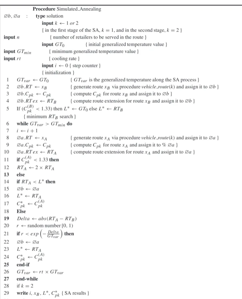
pseudo-code of the Simulated-Annealing procedure is presented in Figure 6.
Another candidate solution∅ais generated using the Monte Carlo routine. IfC(A)
pk < 1.33, it
means that the candidate solution∅ais not feasible. In this case a penalty is applied duplicating the value of RTA (row 12 in Figure 6). Otherwise, ifC(pkA) ≥ 1.33 and RTA < L∗, it means
that a feasible and better solution has been obtained. In such a case the temporary optimum solution so far is∅a, and consequently one makes∅b=∅ato proceed to a new computational
step (rows 15, 16, and 17, Figure 6), and the SA routine reduces the value of the generalized temperature (row 26).
It may occur that the candidate solution∅a is feasible (withC(pkA) ≤ 1.33) but RTA ≥ L∗,
random number 0≤r≤1, one compares the value of r with the analogue Boltzmann probability factor (row 21, in Figure 6). If the inequality in row 21 is observed, the SA accepts ∅a and
consequently one makes ∅b = ∅a to proceed to a new computation procedure (rows 22, 23, and 24, Figure 6), and the SA routine reduces the value of the generalized temperature (row 26). Otherwise, the value of the generalized temperature is reduced (row 26) and a new SA iteration is performed. According to this rationale, if the inequality condition in row (21) is satisfied, a worse (i.e., with RTA ≥ L∗), but feasible solution (i.e.,C(pkA) ≥ 1.33) is accepted in order to
avoid local minima. Otherwise, the former solution is maintained as provisional optimum so far, and the computation proceeds further to a new iteration.
The stage 1 ends whenGTvar ≤GTmin. In the second stage, the initial candidate solution is not
selected at random, but it is just the sub-optimal solution obtained in stage 1.
6.3 SA convergence
As indicated in Section 5.2, four different stage types along the vehicle route are considered: (I) outbound line-haul, which corresponds to the vehicle displacement from the depot to the first visiting retail outlet; (II)product dischargeat retailer premises; (III)local vehicle travelfrom a visited retail outlet to the next one; (IV)inbound line-haul, corresponding to the travel from the last served client back to the depot.
On CoolVan basic results, a mathematical expression to represent the step-by-step internal vehi-cle temperature variation along the route was calibrated (Section 5.2). In the sequel, a computer program evaluates the vehicle internal temperature at one-minute intervals for each route setting defined in the SA routine. For each route, the simulation produces a complete TTI set, and the resultingCpkvalues and total distance D travelled by the vehicle are registered.
The value of constantβ in Eq. (15) depends on the type of stage along the route. For stage-types (I), (III), and (IV) the vehicle is travelling with the cargo door shuttled and the refrigeration system on, and consequentlyβ < 0, since the temperature tends to decrease with time due to the refrigerating process. For stage-type (II) the cargo door stays opened and the refrigeration system is off. The refrigeration system is turned down in such situations to avoid vehicle exhaust pollutants to penetrate the refrigerated compartment, thus spoiling the product. As a consequence
β ≥0.
One important aspect to be considered in SA applications is the convergence of the iterative process (Mengersen & Tweedie, 1996; Holden, 1998; Souza de Cursi & Sampaio, 2012). As mentioned before, in iterative improvement heuristics used to minimize the objective function of a given problem a candidate solution along the process is rejected only when the resulting value of the cost function is not smaller than the previous iterative result. In practice, the dynamics involved in such routines concentrate the search in the neighbourhood of the actual investigated point. The Metropolis-Hastings method, on the other hand, accepts eventual and controlled degradations on the value of the cost function in accordance to a probability evaluation (Souza de Cursi & Sampaio, 2012). From row (21) in Figure 6 one has
Prob(accepting a degradation Delta)=exp
−Delt a GTvar
Procedurevehicle route(k)
1 ifk=1then
{fully randomized routing sequence, except for the depot inserted in positionn+1} 2 fori=1 tondo
3 OK[i] ←true 4 fori=1 tondo 5 flag←false 6 while notflag do
7 j←0
8 while(j=0)do 9 r←random[0,1] 10 j←trunc(r×n+0.5)
11 end-while
12 if(j>0)and(OK[j] =true)then
13 begin
14 flag←true
15 OK[j] ←true
16 x[i] ←j
17 end-if
18 end-while
19 end for
20 x[n+1] ←n+1 21 ifk=2then
{locally randomized routing sequence, except for the depot maintained in positionn+1}
22 fori=1ton+1 23 x[i] ←∅b.x[i]
24 flag←false 25 while notflagdo 26 r←random[0,1] 27 i1←trunc(r×n+0.5) 28 if(i1>0)thenflag←true
29 end-while 30 flag←false 31 while notflagdo 32 r←random[0,1] 33 i2←trunc(r×n+0.5)
34 if(i2>0)and(i2←i1)thenflag←true
35 end-while 36 ℓ←x[i1] 37 x[i1] ←x[i2] 38 x[i2] ←ℓ 39 ∅b.x[i] ←x[i]
40 end-procedure
ProcedureSimulated Annealing
∅b,∅a : typesolution inputk←1or2
{in the first stage of the SA,k=1, and in the second stage,k=2}
inputn {number of retailers to be served in the route}
inputG T0 {initial generalized temperature value}
inputG Tmin {minimum generalized temperature value}
inputr t {cooling rate}
inputi←0{step counter} {initialization}
1 G Tvar ←G T0 {G Tvaris the generalized temperature along the SA process}
2 ∅b.RT←xB {generate routexBvia procedurevehicle route(k)and assign it to∅b} 3 ∅b.Cpk←Cpk {computeCpkfor routexBand assign it to∅b}
4 ∅b.RT ex←RTB {compute route extension for routexBand assign it to∅b}
5 If(C(pkB)<1.33)thenL∗←G T0elseL∗←RTB {minimumRTBsearch}
6 whileG Tvar>G Tmindo
7 i←i+1
8 ∅a.RT←xA {generate routexAvia procedurevehicle route(k)and assign it to∅a}
9 ∅a.Cpk←Cpk {computeCpkfor routexAand assign it to %∅a}
10 ∅a.RT ex←RTA {compute route extension for routexAand assign it to∅a}
11 ifC(pkA)<1.33then 12 RTA←2×RTA
13 else
14 ifRTA<L∗then
15 ∅b←∅a 16 L∗←RTA
17 C∗pk←C(pkA) 18 Else
19 Delta←abs(RTA−RTB)
20 r←random number[0,1)
21 ifr<ex p−G TDelt a
var
then
22 ∅b←∅a 23 L∗←RTA
24 C∗pk←C(pkA) 25 end-if
26 G Tvar ←r t×G Tvar
27 end-while 28 ifk=2
29 writei,xB,L∗,C∗pk{SA results}
30 end-procedure
Souza de Cursi & Sampaio (2012) presented the following theorem: if{Ui}is a sequence of
random variables respecting
Un+1=Un, withn ≥0, and (18)
Un>m, (19)
such that
Prob(Un+1>Un)≤ϑnwith +∞
n=0
ϑn<∞, (20)
the sequence converges to
Un →m. (21)
With decreasing values ofGTvar, the probability of accepting a degradation Delta, given by (17),
satisfies conditions (18), (19) and (20), leading to the convergence of the Metropolis-Hastings method. In fact, such theorem gives a sufficient but not necessary condition, but the practical result is that the Metropolis-Hastings method has shown to be efficient in solving a large number of practical problems (Souza de Cursi & Sampaio, 2012).
Furthermore, regarding the specific problem treated in this work, the temperature inside the ve-hicle tends to increase during the product discharge stage, and tends to decrease during the trav-elling phases. But, since the discharging times are assumed invariable in this analysis, the impact of phase (2) in the optimization process is nil. The same happens with phases (I) and (IV), which also have a fixed behaviour in this analysis. Therefore, the only degrees of freedom when search-ing for the optimum occurs when the vehicle is travellsearch-ing from one visit to the next. In other words, the only phase that opens a way to improve the optimization results is phase III (the vehicle travelling phase). Since the mass m of the product inside the vehicle decreases during visiting stops, the value of exp
β(Tj−mTj−1) j
in expression (15) tends to decrease at every SA step, becauseβ ≤ 0 and mhas a decreasing value as j increases. In conclusion, the probabil-ity of accepting a degradationDelta, given by (17), satisfies conditions (18), (19) and (20), and therefore the SA tends to converge rapidly in our application.
7 RESULTS AND RESEARCH PROSPECTS
7.1 Simulated annealing results
Applying the SA procedures described in Figures 5 and 6, the first SA stage involved 1,306 steps, leading to the following sub-optimal solution:
Routing sequence→Depot – 8 – 10 – 7 – 4 – 3 – 1 – 6 – 12 – 5 – 11 – 9 – 2 – Depot Total distance travelled→241.0 km,Cpk =1.58;
The second SA stage, which departed from the former solution, involved 10,815 steps, leading to the final optimal solution
The model was programmed in Free Pascal, version 2.6.4, to be later incorporated in a Delphi format. It runs in a HP Pavilion dm4-2095br notebook. The first and the second stages of the SA algorithm take 4 and 21 sec respectively to run.
The route with minimum vehicle travel distance is the TSP one, with 204.1 km. But this route presentedCpk =0.35, well bellow the standard level. Taking the inverse TSP route, the PCI is
even worse, withCpk =0.15. The solution obtained with the SA heuristic has shown an increase
of 18.6 km when compared with the TSP configuration, a distance 9.1% greater, but maintaining the refrigerated product within the required temperature range. The SA resulting route is shown in Figure 7, which can be compared with the TSP alternative route. Figure 8, on the other hand, depicts the histogram of the TTI series obtained for the optimal SA solution (as compared with Figure 3, corresponding to the TSP alternative). It can be seen that the temperature distribution is also skewed, justifying the use of theCpkindex (Section 4). The TTI data used to make Figure 8
do not include the values corresponding to the vehicle travel from the last visit back to the depot because the truck is empty along that segment of the route, and therefore the corresponding temperature values do not affect the product quality.
7.2 Sensitivity analysis
For the SA optimal solution indicated in Section 7.1, the values ofCpk were computed for the
intermediate stages of the process and shown in Table 3. As mentioned, the stages correspond to the end of the cargo delivery phases. The results of the model show that the thermal properties inside the vehicle are very sensitive to time variations along the route, specifically the cargo discharging times. This happens due to various real problems as, for example, waiting times to start the unloading process, long paths to reach the point where the discharged cargo is to be set inside the client’s premises, excessive product checking time, etc. On the other hand, the vehicle travelling times, both along the line-haul segments and along the local links between clients in the route, show comparatively less variation.
Since there are an expressive number of variables in the problem, it was adopted the coefficient of variation of the vehicle unloading times to perform a preliminary sensitivity analysis of the results, the coefficient of variation(CV)being the ratio between the standard variation and the expected value. For the outbound and inbound line-haul phases, as well as for the local vehicle displacement times between successive visits, it was assumed CVL H = 0.1. For the cargo
discharging times, on the other hand, a parametric analysis was performed withCVDT varying
from 0.05 to 0.60. Of course, as observed in Table 3, each client shows a particular behaviour in terms ofCpk values. Therefore the sensibility analysis was performed separately for the 12
clients.
Through a Monte Carlo simulation, the model estimates, for each situation, the probability of Cpk <1.33, as a function ofCVDT, displayed per visiting sequence. In Table 4 and in Figure 9,
Figure 7– The SA optimized route as compared to the initial TSP route.
Figure 8– SA optimal route: histogram of internal vehicle temperature.
real configuration, with more detailed discharge-time statistical data collected from each client, this analysis can be performed with more accuracy.
Table 3– Optimal SA route:Cpkvalues for each process stage.
Elapsed time Stage Client no. since departure Cpk
(min)
1 8 157 2.16
2 7 185 2.29
3 4 204 2.34
4 6 222 2.39
5 9 239 2.44
6 10 259 2.47
7 11 282 2.46
8 3 306 2.42
9 12 330 2.37
10 5 355 2.23
11 2 376 1.91
12 1 394 1.33
Table 4– Probability of occurringCpk<1.33 as a function ofCVDTand the visiting sequence.
Visiting Client CVDT – Coefficient of variation, vehicle unloading times sequence number 0.05 0.10 0.15 0.20 0.30 0.40 0.50 0.60
1 8 0 0 0 0 0 0.01 0.02 0.17
2 7 0 0 0 0 0 0.01 0.02 0.17
3 4 0 0 0 0 0 0.02 0.04 0.25
4 6 0 0 0 0 0.01 0.02 0.04 0.25
5 9 0 0 0 0 0.03 0.05 0.09 0.25
6 10 0 0 0 0.01 0.07 0.11 0.17 0.33
7 11 0 0 0 0.03 0.12 0.22 0.27 0.42
8 3 0 0 0.02 0.08 0.21 0.33 0.39 0.58 9 12 0 0.01 0.06 0.13 0.28 0.42 0.50 0.75 10 5 0 0.04 0.09 0.23 0.37 0.49 0.59 0.75 11 2 0.01 0.11 0.16 0.37 0.49 0.61 0.67 0.75 12 1 0.31 0.40 0.49 0.54 0.62 0.72 0.75 0.83
7.3 Conclusion and research prospects
opti-Figure 9– Probability of not satisfying the thermal requirementCpk ≥1.33, as a function ofCVDT.
mized with a Simulated Annealing algorithm in which the objective function to be minimized is the vehicle travelled distance, but respecting a minimum capability index target value.
The authors intend to research further on this subject considering a larger refrigerated cargo distribution problem and using an irregular fleet of vehicles, including smaller trucks, with each one performing more than one route in a working day, the vehicles getting back to the depot when a visiting tour is finished and performing other visiting delivery sequences, as in Oswald & Stirn (2008). Such scheme will possibly improve the overall thermal performance of the delivery system, although with somewhat higher operating costs.
Second, additional TTI data will be gathered with the CoolVan simulator, in order to improve the regression fittings representing the TTI variation. Finally, a dynamic version of this cold-chain distribution planning problem will be developed considering other possible time deviations that might deserve routing revisions. For example, unexpected delays in the cargo unloading activities, traffic delays, and other fault occurrences that will be dynamically incorporated into the model in such a way as to devise corrective real-time measures.
ACKNOWLEDGMENTS
REFERENCES
[1] AARTSEHL & KORSTJHM. 1989. Boltzmann machines for travelling salesman problems. Euro-pean Journal of Operational Research,39: 79–95.
[2] ALVAREZG & FLICKD. 1999. Analysis of heterogeneous cooling of agricultural products inside beans Part II: thermal study.Journal of Food Engineering,39: 239–245.
[3] ANDREE´ S, JIRAW, SCHWINDK-H, WAGNERH & SCHWAGELE¨ F. 2010. Chemical safety of meat and meat products.Meat Science,86: 38–48.
[4] BORCH E & ARINDERP. 2002. Bacteriological safety issues in red meat and ready-to-eat meat products, as well as control measures.Meat Science,62: 381–390.
[5] BREEDAMAV. 1995. Improvement heuristics for the vehicle routing problem based on simulated annealing.European Journal of Operational Research,86: 480–490.
[6] CAMPANONE˜ LA, GINERSA & MASCHERONIRH. 2002. Generalized model for the simulation of food refrigeration. Development and validation of the predictive numerical method.International Journal of Refrigeration,25: 975–984.
[7] CHANGYS & BAIDS. 2001. Control charts for positively-skewed populations with weighted stan-dard deviations.Quality and Reliability Engineering International,17: 397–406.
[8] CHANGYS, CHOIIS & BAIDS. 2002. Process capability indices for skewed populations.Quality and Reliability Engineering International,18: 383–393.
[9] CHENJP & DINGCG. 2001. A new process capability index for non-normal distributions. Interna-tional Journal of Production Research,38(6): 1311–1324.
[10] COOLVANMANUAL– VERSION3.0. 2000. FRPERC – Food Refrigeration & Process Engineering Research Centre, University of Bristol, UK.
[11] CORREIAMH, OLIVEIRA JF & FERREIRA JS. 2000. Cylinder packing by simulated annealing.
Pesquisa Operacional,20(2): 269–286.
[12] CUESTAJF, LAMUA´ M & MORENOJ. 1990. Graphical calculation of half-cooling times.Int. J. Refrigeration,13: 317–324.
[13] CZARSKIA. 2008. Estimation of process capability indices in case of distribution unlike the normal one.Archives of Materials Science and Engineering,34(1), 39–42.
[14] DAELMANJ, JACXSENSL, DEVLIEGHEREF & UYTTENDAELEM. 2013. Microbial safety and quality of various types of cooked chilled foods.Food Control,30: 510–517.
[15] ELLOUZEM & AUGUSTINJ-C. 2010. Applicability of biological time temperature integrators as quality and safety indicators for meat products.International Journal of Food Microbiology,138: 119–129.
[16] ESTRADA-FLORESS & TANNERD. 2005. Interpretation of the Australian Standard for the thermal testing of refrigerated vehicles. EcoLibrium, November 2005, pp. 24–31.
[17] ESTRADA-FLORESS & EDDYA. 2006. Thermal performance indicators for refrigerated road vehi-cles.Int. J. Refrigeration,29: 889–898.