SCHEDULING COPPER REFINING AND CASTING OPERATIONS BY MEANS OF HEURISTICS FOR THE FLEXIBLE FLOW SHOP PROBLEM
Lorena Pradenas
1*, Abel Campos
2, Jes´us Salda˜na
3and V´ıctor Parada
4Received October 7, 2008 / Accepted April 18, 2011
ABSTRACT.Management of the operations in a copper smelter is fundamental for optimizing the use of the plant’s installed capacity. In the refining and casting stage, the operations are particularly complex due to the metallurgical characteristics of the process. This paper tackles the problem of automatic scheduling of operations in the refining and casting stage of a copper concentrate smelter. The problem is transformed into a flexible flow shop problem and to solve it, an iterative method is proposed that operates in two stages: in the first stage, a sequence of jobs is constructed that configures the lots, and in the second, the constructed solution is improved by means of simulated annealing. Fifteen test problems are used to show that the proposed algorithm improves the makespan by an average of 9.42% and the mean flow time by 12.19% with respect to an existing constructive heuristic.
Keywords: refining and casting, flexible flow shop, simulated annealing.
1 INTRODUCTION
In a copper concentrate smelter, a flow of wetsulfide oreis received, and through a metallurgical process, copper is produced. The process involves various typical operations, such as the storage and preparation of the load, melting, conversion, refining and casting, removing slag, and ab-sorption of gases. In the first operation, the wet ore is dried in a rotary furnace, and in smelting, the dry ore is fed into reactors where it is subjected to high temperatures to purify it. As a result, blister copper is obtained that contains 62 to 75% copper, which is the raw material for the con-version operation in which a new purification process gives rise to a product that contains about
*Corresponding author
1Industrial Engineering Department, University of Concepcion, Casilla 160-C, Correo 3, Concepci´on, Chile. E-mail: [email protected]
2Industrial Engineering Department, University of Concepcion, Casilla 160-C, Correo 3, Concepci´on, Chile. E-mail: [email protected]
3Industrial Engineering Department, University of Concepcion, Casilla 160-C, Correo 3, Concepci´on, Chile. E-mail: [email protected]
99% copper (Pradenas, Z´u˜niga & Parada, 2006). In the refining and casting stage, the product of the conversion is again purified in a rotary furnace and is then poured into casting wheels, generating 99.7% pure copper, which represents the final product.
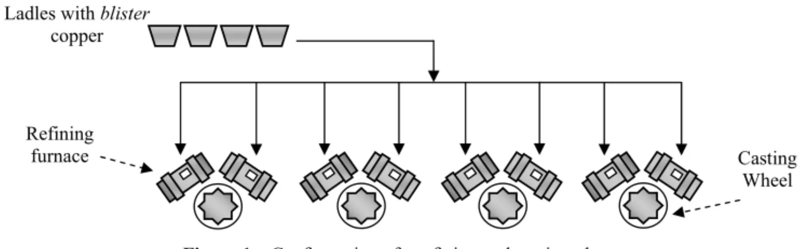
The smelted copper concentrate from the conversion stage is transported and fed to the refining furnaces by means of large ladles moved by a bridge crane. Figure 1 is an operations diagram of a refining and casting plant in which the furnaces are next to each casting wheel, providing independent loads. The refining operation is conducted in a set of reactors of different capacity. To load a given refining reactor, it must be in operation, it must not be processing another load, and a certain amount of time must have passed since it was unloaded. The processing time in this stage depends on the content of the material in the furnace and on its chemical characteristics, and therefore, it is known beforehand.
Copper anodes are cast in fixed molds inserted in rotating casting wheels. The molds in a wheel are filled from a pair of refining furnaces next to the casting wheel, but at the time of filling, only one furnace can be operated. The casting wheel turns periodically and sets up other molds to be filled. As the wheel turns, the filled molds are cooled with water until they reach the sector where they are unloaded automatically.
Ladles with copper
Refining
furnace Casting
Wheel
Figure 1– Configuration of a refining and casting plant.
for a copper concentrate smelter. In their work, they mention that the problem can be consid-ered to belong to the family of scheduling problems, but the topic was not explored further. The problem’s characteristics place it within the scheduling family of problems, which in general are still a great intellectual challenge because of their NP-hardness in most cases (Pinedo, 2008). In this paper, we propose that RCSP can be transformed into a flexible flow shop problem, one of the most extensively studied cases in recent literature on scheduling, but in this particular case taking into account the particular constraints associated with the metallurgical process (Fattahi, Jolai & Arkat, 2009; Mati, Lahlou & Dauzere-Peres, 2011). The computational difficulties that arise when solving instances of this problem numerically have led to attempts to use var-ious techniques to find good quality approximate solutions (Li, Pan, Suganthan & Chua, 2011; Rajkumar, Asokan, Anilkumar & Page, 2011; Zhang, Gao & Shi, 2011). To approach RCSP, we propose a mathematical model and an algorithm to solve it. We develop a computational experiment considering real operating situations.
Section 2 presents a mathematical model of the refining process with its particular constraints. In Section 3, the problem is characterized, a hierarchical approach is established to solve the problem, and an initial solution is improved by simulated annealing in the search for better feasible solutions. Section 4 presents the results and parameterization, and finally, Section 5 gives the main conclusions.
2 MATHEMATICAL REPRESENTATION OF A COPPER REFINING
AND CASTING PLANT
According to the characteristics of this production system, some elements are seen that allow the problem to be associated with a flexibleflow shoptype configuration (Pinedo, 2008):
• A job that enters the system has the possibility of continuing at any of the available work centers,i.e., for each stage of the process a job can be processed on any of the machines available at the job centers, characterizing a flexible type configuration (Bagchi, Gupta & Sriskandarajah, 2006).
• When a job’s process is finished in the refining furnace, it takes a unidirectional flow toward the adjacent casting wheel.
• The machines available at each stage of the process are identical, as they have the same processing speed.
The mathematical model for the problem is constructed with binary integer variables and continu-ous variables following the strategy that has typically been used to represent scheduling problems (Blazewicz, Dror & Weglarz, 1991). The model is presented in equations (1-10).
Parameters
to be processed atq job centers. Parameter pi corresponds to the refining time of jobi, which is a group of ladles with blister copper (in a range of 4 to 6 ladles) that are loaded in a refining furnace. The refining time depends mainly on the concentrate’s composition. The arrival timeri is obtained from estimates of when the loads will come from the previous conversion stage and considers the time required to transfer the ladles that determine jobito the refining furnace. The casting timeci depends mainly on the amount of loaded material. Parameter S represents the time required to prepare the wheel before starting a new casting, and A represents the cleaning time of a refining furnace.
pi = refining time of jobi, ci = casting time of jobi,
ri = time of release or arrival of jobi, S = preparation time of the casting wheel, A = preparation time of the furnace after a casting, E N C = number of allowed linkages.
Decision variables
The decision variables used in the model belong to three groups, some binary, some continuous, and some integer. These variables are related to each other and were selected for convenient formulation of the operating constraints. The binary variablexi jk takes a value of 1 when jobiis the jthjob processed on machinek. In this way each job assigned to a machine has a route and a
position j that delivers the sequence in which it will be processed. Variabletkj denotes the time at which the process of the jthjob of the sequence corresponding to machinekbegins. Variable mkcorresponds to the number of jobs assigned to machinek.
xi jk = 1 if jobi is the jthjob processed on machinek, and 0 in any other case;
tkj = starting time of the jthjob on machinek;
mk = number of jobs assigned to machinek.
Auxiliary variables
ykjl=1 if j=1 (linkage of the jobs processed onkandk+1) and 0 in any other case. Linkage occurs when a wheel finishes processing a job at the same instant at which one of the associated furnaces finishes the refining process; then, it is possible to load the wheel again without any prior preparation. The number of linkages per wheel in the real problem is limited because the workers are exposed to elevated temperatures, causing them to become physically exhausted. For that reason, only one linkage per wheel is generally allowed in a daily schedule.
Objective function and constraints
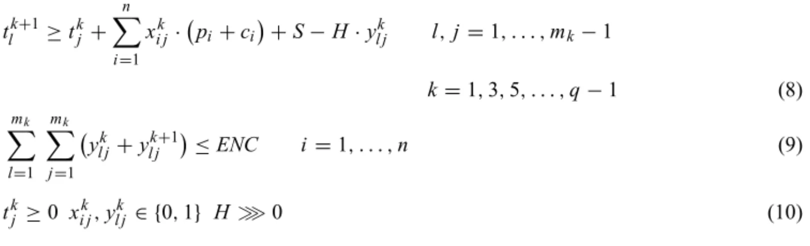
Constraint (2) establishes that for every machine there is a set of jobsmk and that their sum is equal to the total number of jobs(n)to be processed in the system. The group of constraints (3) states that a job does not start its process if it has not arrived at the refining stage(ri), causing the time at which jobi that is in the jth position on machinekstarts being processed to be greater
than or equal to the time of its arrival. Constraint (4) forces all the jobs to be processed in some machinekand in a given position j. Constraint (5) forces at least one of the jobs to be processed in the jthposition on machinek. Constraint (6) restricts the sequence of jobs on one machine, preventing them from interrupting each other. Constraint (7) allows a linkage to be produced in a wheel when a particular condition is fulfilled. If that condition is not fulfilled, constraint (8) allows a new process to be started on the machine after the processing of the previous job has been finished and the corresponding casting wheel has been cleaned. Constraint (9) limits the number of linkages that can be produced in the scheduling of a wheel. Finally, constraint (10) shows the general definition of the model’s variables.
The general precedence constraints are forced by the entry constraints of the jobs to the furnaces and by the double use of the wheel by contiguous furnaces. Under normal operating conditions, a typical refining and casting plant has 4 conversion reactors, 6 refining furnaces, and three casting wheels that maintain 20 hours of effective operation daily. With these facilities, a plant processes approximately 72 blister copper ladles consolidated in 12 jobs, so the possible routing combinations of the jobs are on the order of 612and the operating constraints number 948.
MinZ = Max l<k<m
mk−1
X
j n X
i
xi jk ·tkj+1−tkj+ n X
i
kki mk·(pi +ci) (1) s.t. q X k=1
mk =n (2)
tkj − n X
i=1
xki j·r≥0 j=1, . . . ,mk k=1, . . . ,q (3)
q X k=1 mk X j=1
xi jk =1 i =1, . . . ,n (4)
n X
i=1
xi jk ≤1 j =1, . . . ,mk k=1, . . . ,q (5)
tkj+1≥tkj + n X
i=1
xi jk · pi+ci +A j =1, . . . ,mk−1 k=1, . . . ,q (6)
tlk+1≥tkj + n X
i=1
xi jk · pi+ci− n X
i=1
xilk+1·pi−H· 1−yl jk
l,j =1, . . . ,mk−1
tlk+1≥tkj + n X
i=1
xi jk · pi+ci+S−H·yl jk l,j =1, . . . ,mk−1
k=1,3,5, . . . ,q−1 (8)
mk
X
l=1
mk
X
j=1
yl jk +yl jk+1
≤ENC i=1, . . . ,n (9)
tkj ≥0 xi jk,yl jk ∈ {0,1} H≫0 (10)
Representation of the problem through a graph
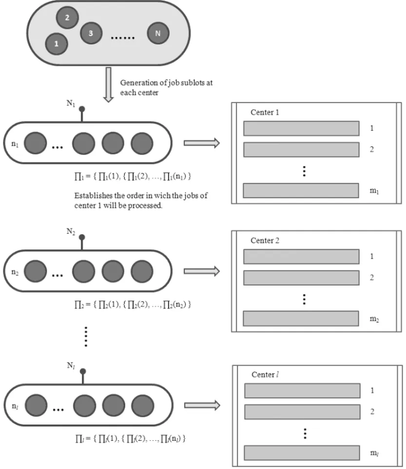
Typically, a flow shop problem is represented with a directed graph (Balas, 1969; Nowicki & Smutnicki, 1998). However, in this case, two particularities of the problem must be taken into account: the concept ofbatchorvirtual batchand thejob processing order. Starting from the unloading of the conversion reactors, the copper ladles are grouped (4 to 6 ladles) into jobs that enter the refining and casting stages associated with their corresponding unloading at different arrival times. Thus, a job constitutes a virtual processing lot,i.e., the jobs are not necessarily available and stored physically one after another in a space or buffer of the plant, but rather, the purpose of their grouping is to allow the definition of virtual job sub-batches before each processing center (routing – sequencing), allowing the scheduling problem to be decomposed at the level of each center, as represented schematically in Figure 2.
Figure 2– Directed graphG(14,3,6)with 6 jobs and 3 processing centers.
3 SOLUTION PROCEDURES
machines are identical; thus, a batch is not associated with a specific center. Each centerlhas a set of jobsNl of sizenl. The processing order of the jobs of each batch Nlcan be expressed as a permutationQ
l = { Q
l(1), Q
l(2), . . . , Q
l(nl)}whereQl(p)denotes the element belonging to sublotlthat will be processed in position p. Figure 3 presents a schematic diagram with the methodology used for the refining and casting plant.
The makespan of the process corresponds to the maximum time for completing a job that is in position pofsublot l. Let us consider that each job has an associated furnace-wheel processing time in the job center, soplidenotes the processing time at centerlof jobi. Therefore, a recursive function can be established for the completion time of a job in a sublotC1,5l(p):
C1,5l(p)=
max
C1,5l(p−1),a5l(p) +pl,5l(p) Unlinked job (11a)
maxC1,5l(p−1),r5l(p),a5l(p) +pl,5l(p) Linked job (11b)
where, p is in the discrete set {1,2,3, . . . ,nl}andCl,5l(0) = 0. a5l(p) is the elapsed time
between the output of the conversion stage and the arrival to the refining and casting stage. The process time pl,5l(p) corresponds to the refining time(r)plus casting time(m)of the job of
sublotlthat is in position p,i.e.:
pl,5l(p)=r5l(p)+m5l(p) (12)
The completion time of a job for centerl in position p starts when the previous job is finished (positionp−1 of sublotl) provided the job has arrived (positionp), which is why the maximum of those two times are in equation (11).
Cmax=MaxC1,5l(p) (13)
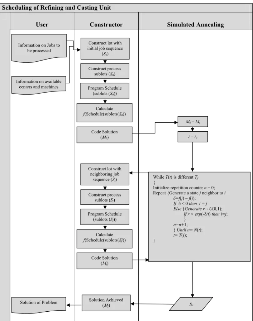
Another approach used to solve the FFSP decomposes the problem into two levels: a routing sub-problem and a job shop sub-problem (Brandimarte, 1993). For the routing sub-problem, we developed a job assignment heuristic forming sublots for each processing center starting from a given job sequence. Job sequencing is initially determined with a heuristic based on the LPT dispatch rule (Pinedo, 2008), and at the later stage, simulated annealing (Kirkpatrick Jr & Vecchi, 1983; Talbi, 2009) is used. A diagram of the procedure’s stages is presented in Figure 6. The construction function generates the processing sublots and schedules the sublot jobs inside a center. The sublots are constructed by assigning each job to a processing center according to the procedure presented in Figure 4. On the other hand, to construct the job schedule of a sublot each job is assigned to some machine of the processing center according to the procedure described in Figure 5.
The representation of the subproblem for the simulated annealing method requires the generation of a solution neighboring the current solution. For that purpose, a position pof the job sequence is chosen randomly, and the neighboring solution is obtained from random exchange among the positions p by p−1 or else p by p+1. The new sequence of jobs generates new sublots for each processing center, and the new starting time of each job must be recalculated.
Procedure 1: Construction of sublots Start
Givena sequence of jobs to be processed;
Whilethere is some unassigned job in the sequence Searchfor an available processing center Ifthere is an unoccupied center;
Assign the job to a center Otherwise
Assign the job to the tail of the center that is set free first
End.
Figure 4– Construction stage of Sublot scheduling.
Procedure 2: Job scheduling Start
For eachof the sublots associated with the centers;
Whilethere is a job of the sublot that has not been scheduled Choose the first job of the sublot
Searchfor an available machine in the center If the center has a machine
Ifthe machine is unoccupied
Schedule the starting time of the job(Ti) Schedule the completion time(Tf)
Otherwise
FollowingTi of sublot=Tf−1+Tsetup wheel Schedule its completion time(Tf)
Otherwise
Choose a machine available at the center Ifthere is an unoccupied machine
Schedule its starting time of the job(Ti) Schedule its completion time(Tf)
Otherwise
If there is linkage
FollowingTiof sublot=Tf−1−Trefining next job Schedule its completion time(Tf)
If there is no linkage
Tifollowing sublot=Tf−1+Tsetup wheel Schedule its completion time(Tf)
End while; End for;
End.
Solution of Problem Solution Achieved ( ) Construct lot with
neighboring job sequence ( )
Construct process sublots ( )
Program Schedule (sublots ( ))
Calculate (Schedule(sublots( ))
Code Solution ( )
=
=
While ( ) is different {
Initialize repetition counter = 0; Repeat {Generate a state neighbor to
( ) ( ); < 0
{ (0,1); ( ) ; }
1; } ( );
( ); }
Information on Jobs to be processed
Information on available centers and machines
Construct lot with initial job sequence
( )
Construct process sublots ( )
Program Schedule (sublots ( ))
Calculate (Schedule(sublots( ))
Code Solution ( )
Figure 6– Interaction between the Construction and Simulated Annealing.
4 RESULTS 4.1 Test problems
To generate the test problems, a computational tool was executed that programs the activities in the conversion plant, which is the previous stage in copper production (Pradenaset al., 2006). The output of this tool produces the input data for the copper refining and casting problem. This information contains data on the instant at which each ladle with molten material is produced in the conversion stage. One RCSP instance is defined by the number of jobs that will be pro-cessed, the availability of the processing centers, and the arrival and processing times of each. To generate the test problems, the normal operation of a refining and casting plant is considered, and alterations are made as to the availability of the processing centers and the number of jobs to be processed, increasing the complexity of the real problem instances. Table 1 presents the characteristics of the generated instances and the available centers.
Table 1– Characteristics of the jobs.
Problem No. of Consolidated Available
instances jobs centers
RM08XX 5 8 3
RM10XX 5 10 3
RM12XX 5 12 3
For each of the five instances of the three types of problems, refining, casting, arrival, and loading times were generated randomly with a uniform triangular probability distribution, as presented in Table 2. Time is measured in minutes and load size in metric tons.
Table 2– Distribution of the data that characterize each job.
Data Distribution function Refining Time Uniform [130,175]
Casting Time Uniform [240,420] Arrival Time Uniform [30, 1150]
Load Triangular [250, 250, 350]
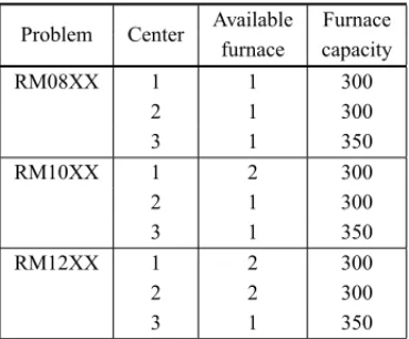
For the studied cases, it is assumed that the processing centers for each type of instance are always available, so that the three casting wheels are always operating and are fed by one of their corresponding refining reactors. Table 3 gives the details.
Hardware used
Table 3– Description of the processing centers.
Problem Center Available Furnace furnace capacity
RM08XX 1 1 300
2 1 300
3 1 350
RM10XX 1 2 300
2 1 300
3 1 350
RM12XX 1 2 300
2 2 300
3 1 350
Parameter definition
The simulated annealing method has various control parameters whose values must be estab-lished so that it will deliver good quality solutions in a reasonable execution time. To achieve an adequate parameterization, use was made of the 15 instances and of the WinCalibra soft-ware, whose procedure is based on aTaguchi Factorial Experiment Design and a local search (Adenso-Diaz & Laguna, 2006). The values obtained from the parameterization are presented in Table 4.
Table 4– Parameter values.
Parameter Range Obtained value
Parameterα 0.090-0.999 0.995
Initial temperature 1000-1700 1175
Final temperature 0.01-10.00 7.5
Iterations for each temperature level 1-100 76
Schedule generation
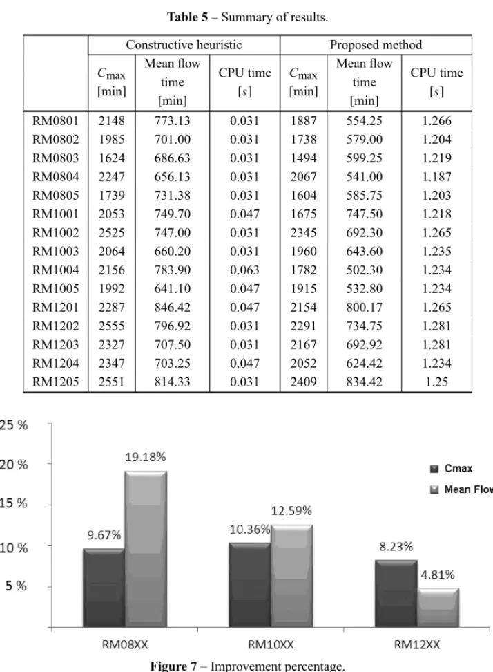
Table 5 shows the results obtained for the 15 instances using the proposed method as well as the constructive heuristic (Pradenaset al., 2005). The completion time(Cmax), the mean flow time, and the CPU time are given for each instance.
The proposed method improvesCmaxby an average of 9.42% and mean flow time by 12.19%
with respect to the constructive heuristic. Even though the CPUtime is very low, it is longer in simulated annealing, consistent with the difference between a constructive heuristic and the iterative characteristics of the simulated annealing metaheuristic. Figure 7 shows the average percentage improvement inCmax and mean flow time for each of the three types of problems
Table 5– Summary of results.
Constructive heuristic Proposed method
Cmax
Mean flow
CPU time Cmax
Mean flow
CPU time
[min] time [s] [min] time [s]
[min] [min]
RM0801 2148 773.13 0.031 1887 554.25 1.266
RM0802 1985 701.00 0.031 1738 579.00 1.204
RM0803 1624 686.63 0.031 1494 599.25 1.219
RM0804 2247 656.13 0.031 2067 541.00 1.187
RM0805 1739 731.38 0.031 1604 585.75 1.203
RM1001 2053 749.70 0.047 1675 747.50 1.218
RM1002 2525 747.00 0.031 2345 692.30 1.265
RM1003 2064 660.20 0.031 1960 643.60 1.235
RM1004 2156 783.90 0.063 1782 502.30 1.234
RM1005 1992 641.10 0.047 1915 532.80 1.234
RM1201 2287 846.42 0.047 2154 800.17 1.265
RM1202 2555 796.92 0.031 2291 734.75 1.281
RM1203 2327 707.50 0.031 2167 692.92 1.281
RM1204 2347 703.25 0.047 2052 624.42 1.234
RM1205 2551 814.33 0.031 2409 834.42 1.25
Figure 7– Improvement percentage.
5 CONCLUSIONS
for each available refining center in such a way that a route and a sequence for entering the refining center are defined that optimize the use of the casting wheel. At the second level, this constructed solution is improved by means of the simulated annealing method. After solving 15 test problems, the proposed algorithm improved on themakespanby 9.42% and the mean flow time by 12.19% with respect to a constructive heuristic.
ACKNOWLEDGMENTS
Authors were supported by projects: CONICYT: FBO16; UDEC-208.97011-1 and by the Mil-lennium Institute Complex Engineering Systems ICM: P-05-004-F.
REFERENCES
[1] ADENSO-DIAZ B & LAGUNA M. 2006. Fine-tuning of algorithms using fractional experimental designs and local search.Operations Research,54(1): 99–114.
[2] BAGCHI TP, GUPTAJND & SRISKANDARAJAHC. 2006. A review of TSP based approaches for flowshop scheduling.European Journal of Operational Research,169(3): 816–854.
[3] BALAS E. 1969. Machine sequencing via disjunctive graphs: an implicit enumeration algorithm. Operations Research,17(6): 941–957.
[4] BLAZEWICZJ, DRORM & WEGLARZJ. 1991. Mathematical programming formulations for ma-chine scheduling: a survey.European Journal of Operational Research,51(3): 283–300.
[5] BRANDIMARTEP. 1993. Routing and scheduling in a flexible job shop by tabu search.Annals of Operations Research,41(3): 157–183.
[6] FATTAHIP, JOLAIF & ARKATJ. 2009. Flexible job shop scheduling with overlapping in operations. Applied Mathematical Modelling,33(7): 3076–3087.
[7] KIRKPATRICK S JR, D GUELAT & VECCHI MP. 1983. Optimization by simulated annealing. Science,220(4598): 671–680.
[8] LIJ, PANQ, SUGANTHANP & CHUAT. 2011. A hybrid tabu search algorithm with an efficient neighborhood structure for the flexible job shop scheduling problem. International Journal of Advanced Manufacturing Technology,52(5-8): 683–697.
[9] MATIY, LAHLOUC & DAUZERE-PERESS. 2011. Modelling and solving a practical flexible job-shop scheduling problem with blocking constraints.International Journal of Production Research, 49(8): 2169–2182.
[10] NOWICKIE & SMUTNICKIC. 1998. The flow shop with parallel machines: A tabu search approach. European Journal of Operational Research,106(2-3): 226–253.
[11] PINEDOM. 2008. Scheduling: theory, algorithms, and systems. Springer Verlag.
[12] PRADENAS L, N ´UNEZ G, PARADA V & FERLANDJ. 2005. Gesti´on de operaciones de refino y Moldeo en la Producci´on de Cobre.Revista Ingenier´ıa de Sistemas,19(1): 19–28.
[14] RAJKUMAR M, ASOKANP, ANILKUMARN & PAGE T. 2011. A GRASP algorithm for flexible job-shop scheduling problem with limited resource constraints.International Journal of Production Research,49(8): 2409–2423.
[15] TALBI EG. 2009. Metaheuristics: From design to implementation. John Wiley & Sons, Hoboken (NJ).