Article
The Urban Heat Island Effect and the Role of
Vegetation to Address the Negative Impacts of Local
Climate Changes in a Small Brazilian City
Elis Dener Lima Alves1,* and António Lopes2
1 Instituto Federal de Educação, Ciência e Tecnologia, Ceres 76300-000, Brazil
2 Institute of Geography and Spatial Planning (IGOT-ULisboa), Center of Geographical Studies—Climate Change and Environmental Systems Research Group, Universidade de Lisboa, 1649-003 Lisboa, Portugal; [email protected]
* Correspondence: [email protected]; Tel.: +55-62-3307-7100 Academic Editor: Robert W. Talbot
Received: 2 November 2016; Accepted: 13 January 2017; Published: 9 February 2017
Abstract:This study analyzes the influence of urban-geographical variables on determining heat islands and proposes a model to estimate and spatialize the maximum intensity of urban heat islands (UHI). Simulations of the UHI based on the increase of normalized difference vegetation index (NDVI), using multiple linear regression, in Iporá (Brazil) are also presented. The results showed that the UHI intensity of this small city tended to be lower than that of bigger cities. Urban geometry and vegetation (UI and NDVI) were the variables that contributed the most to explain the variability of the maximum UHI intensity. It was observed that areas located in valleys had lower thermal values, suggesting a cool island effect. With the increase in NDVI in the central area of a maximum UHI, there was a significant decrease in its intensity and size (a 45% area reduction). It is noteworthy that it was possible to spatialize the UHI to the whole urban area by using multiple linear regression, providing an analysis of the urban set from urban-geographical variables and thus performing prognostic simulations that can be adapted to other small tropical cities.
Keywords:urban climate change; UHI; urban microclimates; mitigation
1. Introduction
The expansion of urban centers over the years has created a marked heating pattern in relation to their rural environment [1–4], especially in densely built urban centers with little vegetation where temperatures tend to be higher [4–9]. This pattern is known as urban heat islands (UHI) [4,10,11]. In 1833, Luke Howard hypothesized that the excess heat in cities during summer was due to a greater absorption of solar radiation by the vertical surfaces of a city and the lack of available humidity for evaporation [11]. Howard’s theories were surprisingly accurate. However, there are several other reasons for the appearance of an UHI pattern: urban heat generated from heating, air conditioning, transportation, and industrial processes [11], and a decrease in wind speed due to a roughness length increase, which also slows down energy transfer from the surface to the urban atmosphere [12,13]. Pollution also contributes to this scenario because air particles absorb and emit heat to urban canyons [14,15].
Several other problems related to UHIs have been observed, such as increased urban pollution, intense summer rainfalls, and high energy consumption. Also, there may be problems related to thermal discomfort and heat stress impacting human health and causing a high death rate of already physically vulnerable people.
Attenuating the effects of UHI in tropical climates is imperative and should be considered a key element in urban design to address climate change in cities [14,16]. Despite its volume, studies of
Atmosphere 2017, 8, 18 2 of 14
urban heat islands have been an important tool to manage urban spaces. As a part of urban planning, spatialization of the differences between intra-urban and rural temperatures can contribute to mitigate the magnitude of UHIs [17,18] and improve quality of life.
Significant efforts have been made by the scientific community to assess the impact of UHIs on the urban environment [4,19–21]: simulations of urban heat islands and multiple linear regression have been used in numerous studies [22–29], obtaining good results. When combined with observations, they may provide prospects for the reorganization of territories. However, as previously pointed out by others, very often the results of studies are not properly used by the government due to a lack of detailed and useful information, or simply due to the lack of interest by urban planners not sufficiently preoccupied with the problems related with urban climate changes [29].
This research is a first UHI assessment in Iporá, and the main objectives are:
(i) to analyze the influence of urban-geographical variables as triggering factors of the formation of heat islands;
(ii) to propose a model to estimate and spatialize the maximum intensity of UHIs in the city core; and (iii) to simulate the mitigation of urban heat islands with an increase in vegetation index (NDVI) by
using multiple linear regression. 2. Materials and Methods
2.1. Data Collection
The city of Iporá is located in the western part of the state of Goiás (GO), Brazil (Figure1), and its territorial area is approximately 1026.4 km2[30]. The population of Iporá has not changed substantially in recent decades (from 1980, there was an increase of approximately 4920 people), and as of the writing of this paper the city currently counts 31,274 inhabitants [30]. From The economy is based on the third sector, followed by agriculture. The rainy season occurs from April to September (with an average of approximately 180 mm), and from October to March (approximately 1400 mm). The mean total annual value is approximately 1600 mm.
spatialization of the differences between intra-urban and rural temperatures can contribute to mitigate the magnitude of UHIs [17,18] and improve quality of life.
Significant efforts have been made by the scientific community to assess the impact of UHIs on the urban environment [4,19–21]: simulations of urban heat islands and multiple linear regression have been used in numerous studies [22–29], obtaining good results. When combined with observations, they may provide prospects for the reorganization of territories. However, as previously pointed out by others, very often the results of studies are not properly used by the government due to a lack of detailed and useful information, or simply due to the lack of interest by urban planners not sufficiently preoccupied with the problems related with urban climate changes [29].
This research is a first UHI assessment in Iporá, and the main objectives are:
(i) to analyze the influence of urban-geographical variables as triggering factors of the formation of heat islands;
(ii) to propose a model to estimate and spatialize the maximum intensity of UHIs in the city core; and (iii) to simulate the mitigation of urban heat islands with an increase in vegetation index (NDVI) by
using multiple linear regression.
2. Materials and Methods
2.1. Data Collection
The city of Iporá is located in the western part of the state of Goiás (GO), Brazil (Figure 1), and
its territorial area is approximately 1026.4 km2 [30]. The population of Iporá has not changed
substantially in recent decades (from 1980, there was an increase of approximately 4920 people), and as of the writing of this paper the city currently counts 31,274 inhabitants [30]. From The economy is based on the third sector, followed by agriculture. The rainy season occurs from April to September (with an average of approximately 180 mm), and from October to March (approximately 1400 mm). The mean total annual value is approximately 1600 mm.
Seven thermo-hygrometers were installed within the urban area of Iporá. The distribution of the thermo-hygrometers sought to meet two criteria: (i) represent the different urban-geographical characteristics of the city; and (ii) standardize the contact surface, following the recommendations by Oke [31]. They were installed in white-painted weather shelters fixed on wooden poles at a height of 1.80 m in roundabouts and road centers (Figure 1) with a SVF ≥ 0.8. With this procedure, it is assured that there is no microclimatic influence of buildings or nearby trees.
Figure 1. Location of the city of Iporá and the measurement sites.
The OM-EL-USB-2-LCD thermo-hygrometers were manufactured by OMEGA. They have an accuracy of 0.5 °C for air temperature. Data was recorded from 20 October 2014 to 24 November 2014, recording data every 30 min, totaling 1630 data outputs.
Figure 1.Location of the city of Iporá and the measurement sites.
Seven thermo-hygrometers were installed within the urban area of Iporá. The distribution of the thermo-hygrometers sought to meet two criteria: (i) represent the different urban-geographical characteristics of the city; and (ii) standardize the contact surface, following the recommendations by Oke [31]. They were installed in white-painted weather shelters fixed on wooden poles at a height of
1.80 m in roundabouts and road centers (Figure1) with a SVF≥0.8. With this procedure, it is assured that there is no microclimatic influence of buildings or nearby trees.
The OM-EL-USB-2-LCD thermo-hygrometers were manufactured by OMEGA. They have an accuracy of 0.5◦C for air temperature. Data was recorded from 20 October 2014 to 24 November 2014, recording data every 30 min, totaling 1630 data outputs.
2.2. Methodology and Data Analysis
There is not an universal criteria for calculating the intensity of urban heat islands [4,31–33]. In many studies, such calculation was performed by subtracting the temperature recorded in the urban area from the temperature recorded at weather stations or airports. For example, this technique was applied for more than 20 years by Alcoforado et al. [4] for the city of Lisbon, Portugal. Miao et al. [1] defined UHI as the mean air temperature difference between stations inside (i.e., urban areas) and outside (i.e., rural areas) built environments.
Based on Lopes et al. [4], it was considered that an UHI occurred in Iporá when the temperature of one of the collection sites was higher than the temperature of the other collection sites. The intensity of an UHI was calculated as the difference, at a given moment, between the site with the highest temperature (Thigher) and the site with the lowest temperature (Tlower), according to Equation (1).
UHIt0 h→23 h=Thigher−Tlower (1)
The urban-geographical variables used for multiple linear regressions were altitude (A), terrain aspect (TA), demographic density (DD), NDVI, terrain slope (TS), and urbanization index (UI). Seven areas were selected (Figure2), corresponding to each measurement site. A square with an area of 40,000 m2(200 m×200 m) focusing on each measurement location was determined (Figure2). Mean and mode values of the urban-geographical variables for each square were determined (Table1).
Atmosphere 2017, 8, 18 3 of 13
2.2. Methodology and Data Analysis
There is not an universal criteria for calculating the intensity of urban heat islands [4,31–33]. In many studies, such calculation was performed by subtracting the temperature recorded in the urban area from the temperature recorded at weather stations or airports. For example, this technique was applied for more than 20 years by Alcoforado et al. [4] for the city of Lisbon, Portugal. Miao et al. [1] defined UHI as the mean air temperature difference between stations inside (i.e., urban areas) and outside (i.e., rural areas) built environments.
Based on Lopes et al. [4], it was considered that an UHI occurred in Iporá when the temperature of one of the collection sites was higher than the temperature of the other collection sites. The intensity of an UHI was calculated as the difference, at a given moment, between the site with the highest temperature (Thigher) and the site with the lowest temperature (Tlower), according to Equation (1).
UHI → = − (1)
The urban-geographical variables used for multiple linear regressions were altitude (A), terrain aspect (TA), demographic density (DD), NDVI, terrain slope (TS), and urbanization index (UI). Seven areas were selected (Figure 2), corresponding to each measurement site. A square with an area of
40,000 m2 (200 m × 200 m) focusing on each measurement location was determined (Figure 2). Mean
and mode values of the urban-geographical variables for each square were determined (Table 1).
Figure 2. Measurement sites and method for obtaining urban-geographical variables.
The normalized difference vegetation index ( NDVI ) and the urbanization index (UI) were calculated using Landsat 5 Thematic Mapper (TM) satellite images.
The NDVI is a simple indicator of vegetation biomass and strength, and can be used as cover fraction using empirical relations as a possible basis function. Normalized Difference Vegetation Index (NDVI) is determined by:
NDVI =NIR − R
NIR + R (2)
where NDVI is Normalized Difference Vegetation Index, NIR is Near InfraRed (band 4 in Landsat 5 TM), and R (Red) is band 3 of the satellite. The Urbanization Index (UI) was determined using Equation (3). The UI is generally used because of its easiness of mapping and characterizing built areas [34,35].
UI =SWIR − R
SWIR + R (3)
where SWIR (Short Wave Infra-Red) is Landsat 5 TM band 7.
Figure 2.Measurement sites and method for obtaining urban-geographical variables.
The normalized difference vegetation index (NDVI) and the urbanization index (UI) were calculated using Landsat 5 Thematic Mapper (TM) satellite images.
The NDVI is a simple indicator of vegetation biomass and strength, and can be used as cover fraction using empirical relations as a possible basis function. Normalized Difference Vegetation Index (NDVI) is determined by:
NDVI= NIR−R
NIR+R (2)
where NDVI is Normalized Difference Vegetation Index, NIR is Near InfraRed (band 4 in Landsat 5 TM), and R (Red) is band 3 of the satellite. The Urbanization Index (UI) was determined using Equation (3). The UI is generally used because of its easiness of mapping and characterizing built areas [34,35].
UI= SWIR−R
SWIR+R (3)
where SWIR (Short Wave Infra-Red) is Landsat 5 TM band 7.
Table 1. Altitude (A), terrain slope (TS), demographic density (DD), NDVI, terrain aspect (TA), and urbanization index (UI) at the measurement sites.
Sites A1 TS1 DD2 NDVI1 TA3 UI1 1 608.3 1 684.4 0.05 213 −0.09 2 570.6 2.4 3560.3 0.26 190 −0.27 3 588.8 2.1 2103 0.07 208 0 4 580.8 2.7 70.6 0.01 296 0.06 5 596.9 3.3 4002 0.08 280 −0.02 6 615.1 1.7 2084.6 0.08 282 0.01 7 595.8 2.4 912.6 0.09 233 −0.02
1Mean value in a square with a 200 m side centered on the measurement site;2Population calculated by the Brazilian Census of 2010;3Mode value in a square with a 200 m side centered on the measurement site.
Multiple linear regression is a multivariate technique whose main purpose is to obtain a mathematical relation between one of the studied variables (dependent or response variable) and the other variables that describe the system (independent or explanatory variables). It also seeks to reduce the number of independent variables with a minimal loss of information. After the mathematical relation is found, its main application is to produce values for the dependent variable when independent variables are available [36].
In order to determine which independent variables had the greatest potential to contribute to UHIs, a step-by-step multiple linear regression was used [37,38].
According to Montgomery, Peck, and Vining [39], the multiple linear regression model (MLRM) with k control variables can be represented by Equation (4).
Y=β0+β1X1i+β2X2i+ · · · +βkXki+εi (4)
The regression coefficients β0, β1, ..., βkare described by Montgomery, Peck, and Vining [39] as follows: β0is the intercept coefficient, which is the average of Yiwhen all control variables are equal to zero; the coefficients β1, ..., βkare partial regression coefficients. The coefficient βkcan be interpreted as a partial derivative of Yiin relation to Xki, that is, the variation of Y caused by a unit change in Xk since the other control variables are kept constant.
The criterion adopted for input and output variables in the model was their significance level (p-value < 0.05). The best multiple linear regression model was used to estimate UHI values for the entire urban area. The software used (Surfer 13) performed a semi-variogram analysis (presented in Section3), followed by the interpolation of UHI using the kriging technique.
Simulations of UHIs were made from the equations obtained by multiple linear regression with several scenarios corresponding to the increase in vegetation cover.
3. Results and Discussion
As previously discussed, a total of 1630 data values (corresponding to the period from 20 October 2014 to 24 November 2016) were used to calculate the value of maximum heat islands.
3.1. A Case Study of a Hot and Dry Night (21 October 2014) in the Iporá Region
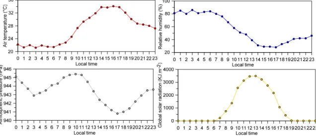
In tropical areas, very hot and dry nights may lead to extremely uncomfortable situations and even to an excess of mortality, especially of more vulnerable people (young and old people). This case study considers one of these situations, which was studied for the first time in the city of Iporá. On 21 October 2014, the Intertropical Convergence Zone (ZCIT) oscillated from 08◦N to 10◦N in the Pacific and from 07◦N to 09◦N in the Atlantic, and a hot and dry continental tropical air mass (mTc) affected the study area. The Brazilian National Institute of Meteorology (INMET) station located on the outskirts of the city (Figure3) recorded an amplitude of 12.9◦C in the air temperature: the minimum (21.2◦C) was recorded at 03:00 and the maximum at 16:00 (34.1◦C). Relative humidity reached less than 30% during several hours, approximately from 14:00 to 17:00. There was little fluctuation in the atmospheric pressure (from 941 to 945 hPa) because a low system influenced the region. However, due to the influence of the mTc air mass, the sky was clear and the global solar radiation was more than 3500 KJ·m−2at noon.
Atmosphere 2017, 8, 18 5 of 13
region. However, due to the influence of the mTc air mass, the sky was clear and the global solar radiation was more than 3500 KJ·m−2 at noon.
Figure 3. Weather data from the Brazilian National Institute of Meteorology (INMET) station on 21 October 2014.
3.2. Multiple Linear Regression of Maximum Heat Islands
In order to observe the pattern of an UHI during its greatest intensity, multiple linear regressions were calculated at 20:30, 21:00, and 21:30 on 21 October 2014. NDVI and UI variables were used in three equations (Equations (5)–(7)) because these are the most important in the model and they represent an effective way to propose measures to address urban climate change. In Equation (5), NDVI explained 92.3% of the spatial variability of the UHI at 20:30, the UI in Equation (6) explained 86.5% at 21:00, and Equation (7) explained 88.4% of the variability of the UHI at 21:30. All equations (Table 2) had a r2 > 0.9. Others urban-geographical areas were not included in the model because they
presented a p-value < 0.05.
Table 2. Equations obtained for maximum urban heat islands (UHI) intensity.
Estimated UHI Number of Equations
UHI : = 29.84 + (0.0000753 × DD) − (13.510 × NDVI) + (0.744 × UI) Equation (5) UHI : = 29.741 − (5.933 × NDVI) − (0.00309 × TA) + (6.478 × UI) Equation (6) UHI : = 28.927 − (7.302 × NDVI) + (5.508 × UI) Equation (7)
The semi-variogram used for kriging UHIs at 20:30 (Figure 4) was an exponential model, with a
r2 = 0.69, a nugget effect = 0.06 ( ), and a silo ( + ) = 1.23. From this point, it is considered that
there is no spatial dependence between samples. The spatial dependence on UHI intensity, obtained by the range ( ) was 188 m. For the kriging of UHI at 21:00, the Gaussian model was used, with r2 = 0.78,
nugget = 0.48, silo = 1.13, and spatial dependence = 295 m (the maximum distance with the influence of space on each point). At 21:30, the best semi-variogram was obtained with r2 = 0.94, = 0.82, and
+ = 2.69. The maximum range of spatial dependence was greater than the others (758 m). The semi-variograms (Figure 4) were used as an input model for the spatialization (with kriging) of UHIs. The resulting maps are shown in Figure 5. The patterns of UHIs were similar for all three times, and the area located at the southwest of the maps shows an intense heat island corresponding to the center of Iporá. Its peak was at 21:30. In addition, the spatial patterns of UHI < 0, also called urban cool islands (UCI), were maintained.
Figure 3. Weather data from the Brazilian National Institute of Meteorology (INMET) station on 21 October 2014.
3.2. Multiple Linear Regression of Maximum Heat Islands
In order to observe the pattern of an UHI during its greatest intensity, multiple linear regressions were calculated at 20:30, 21:00, and 21:30 on 21 October 2014. NDVI and UI variables were used in three equations (Equations (5)–(7)) because these are the most important in the model and they represent an effective way to propose measures to address urban climate change. In Equation (5), NDVI explained 92.3% of the spatial variability of the UHI at 20:30, the UI in Equation (6) explained 86.5% at 21:00, and Equation (7) explained 88.4% of the variability of the UHI at 21:30. All equations (Table2) had a r2> 0.9. Others urban-geographical areas were not included in the model because they presented a p-value < 0.05.
Table 2.Equations obtained for maximum urban heat islands (UHI) intensity.
Estimated UHI Number of Equations
UHI20:30=29.84+ (0.0000753×DD) − (13.510×NDVI) + (0.744×UI) Equation (5) UHI21:00=29.741− (5.933×NDVI) − (0.00309×TA) + (6.478×UI) Equation (6) UHI21:30=28.927− (7.302×NDVI) + (5.508×UI) Equation (7)
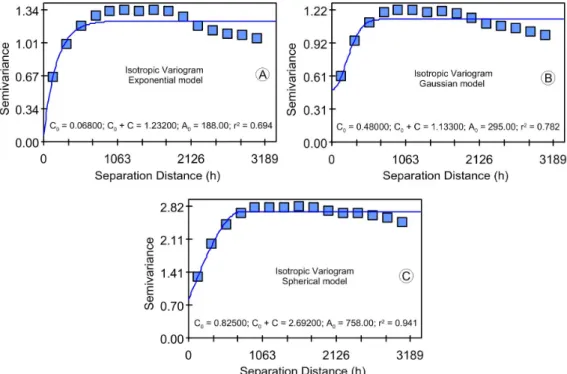
The semi-variogram used for kriging UHIs at 20:30 (Figure 4) was an exponential model, with a r2= 0.69, a nugget effect = 0.06 (C0), and a silo (C0+C) = 1.23. From this point, it is considered that there is no spatial dependence between samples. The spatial dependence on UHI intensity, obtained by the range (A0) was 188 m. For the kriging of UHI at 21:00, the Gaussian model was used, with r2= 0.78, nugget = 0.48, silo = 1.13, and spatial dependence = 295 m (the maximum distance with the influence of space on each point). At 21:30, the best semi-variogram was obtained with r2= 0.94, C0= 0.82, and C0+C = 2.69. The maximum range of spatial dependence was greater than the others (758 m).
Atmosphere 2017, 8, 18 6 of 13
Figure 4. Semi-variograms used for the kriging of the maximum UHI intensities at 20:30 (A);
21:00 (B); and 21:30 (C).
Figure 5. Thermal patterns estimated on the 21 October 2014, at 20:30 (A); 21:00 (B); and 21:30 (C). According to the boxplots (Figure 6), the highest median value was observed for the UHI at 21:30 (2.7 °C), whereas the maximum value was observed at 21:00 (4.5 °C). The highest values corresponding to 50% of the data were observed at 21:30 (2.2–3 °C), while at 20:30 and 21:00 the interval was lower: 1.9–2.8 °C and 1.8–2.8 °C, respectively. Therefore, the data set of boxplots shows that there was little change in the intensity of the UHI.
Urban heat islands are often regarded as the most important factor influencing the urban environment and its surroundings [2,4,40]. However, the phenomenon known as urban cool islands may also occur with significant effects. This pattern was first detected by Hu, Su, and Zhang [41] based on an analysis of microclimate characteristics of a reservoir in the Hexi Region, China. Figure 4.Semi-variograms used for the kriging of the maximum UHI intensities at 20:30 (A); 21:00 (B); and 21:30 (C).
Atmosphere 2017, 8, 18 6 of 13
Figure 4. Semi-variograms used for the kriging of the maximum UHI intensities at 20:30 (A);
21:00 (B); and 21:30 (C).
Figure 5. Thermal patterns estimated on the 21 October 2014, at 20:30 (A); 21:00 (B); and 21:30 (C). According to the boxplots (Figure 6), the highest median value was observed for the UHI at 21:30 (2.7 °C), whereas the maximum value was observed at 21:00 (4.5 °C). The highest values corresponding to 50% of the data were observed at 21:30 (2.2–3 °C), while at 20:30 and 21:00 the interval was lower: 1.9–2.8 °C and 1.8–2.8 °C, respectively. Therefore, the data set of boxplots shows that there was little change in the intensity of the UHI.
Urban heat islands are often regarded as the most important factor influencing the urban environment and its surroundings [2,4,40]. However, the phenomenon known as urban cool islands may also occur with significant effects. This pattern was first detected by Hu, Su, and Zhang [41] based on an analysis of microclimate characteristics of a reservoir in the Hexi Region, China.
Figure 5.Thermal patterns estimated on the 21 October 2014, at 20:30 (A); 21:00 (B); and 21:30 (C).
The semi-variograms (Figure4) were used as an input model for the spatialization (with kriging) of UHIs. The resulting maps are shown in Figure5. The patterns of UHIs were similar for all three times, and the area located at the southwest of the maps shows an intense heat island corresponding
to the center of Iporá. Its peak was at 21:30. In addition, the spatial patterns of UHI < 0, also called urban cool islands (UCI), were maintained.
According to the boxplots (Figure6), the highest median value was observed for the UHI at 21:30 (2.7◦C), whereas the maximum value was observed at 21:00 (4.5◦C). The highest values corresponding to 50% of the data were observed at 21:30 (2.2–3◦C), while at 20:30 and 21:00 the interval was lower: 1.9–2.8◦C and 1.8–2.8◦C, respectively. Therefore, the data set of boxplots shows that there was little change in the intensity of the UHI.Atmosphere 2017, 8, 18 7 of 13
Figure 6. Boxplots of UHIs at 20:30, 21:00, and 21:30.
Even at a maximum UHI, cool islands may occur. This is shown in Figure 7, which was designed by superimposing the UHI over the relief. It can be seen that the areas located in valley bottoms had the lowest values, suggesting a cold air drainage. This is in accordance with the study by Lopes [42], which reported that cold-air lakes in Oeiras, Portugal, formed in topographically depressed areas, were double fed by the cool air formed in situ by irradiation and also by the cold air drained by gravity that formed in the upper sections of the valleys.
Figure 7. Maximum UHI intensities.
Figure 8 shows the quantification of the area of each urban heat island class. The UHI classes > 1 °C had an area of 14.91 km2, which corresponds to 90% of the urban area. The UHI classes < 1 °C had an area of 1.67 km2, which corresponds to 10% of the total area. Therefore, there was a predominance of heat islands in high intensity classes. The cool islands (classes with UHI < 0 °C), were concentrated in the valley bottoms, which present vegetated areas and water bodies (Figure 8).
Figure 6.Boxplots of UHIs at 20:30, 21:00, and 21:30.
Urban heat islands are often regarded as the most important factor influencing the urban environment and its surroundings [2,4,40]. However, the phenomenon known as urban cool islands may also occur with significant effects. This pattern was first detected by Hu, Su, and Zhang [41] based on an analysis of microclimate characteristics of a reservoir in the Hexi Region, China.
Even at a maximum UHI, cool islands may occur. This is shown in Figure7, which was designed by superimposing the UHI over the relief. It can be seen that the areas located in valley bottoms had the lowest values, suggesting a cold air drainage. This is in accordance with the study by Lopes [42], which reported that cold-air lakes in Oeiras, Portugal, formed in topographically depressed areas, were double fed by the cool air formed in situ by irradiation and also by the cold air drained by gravity that formed in the upper sections of the valleys.
Atmosphere 2017, 8, 18 7 of 13
Figure 6. Boxplots of UHIs at 20:30, 21:00, and 21:30.
Even at a maximum UHI, cool islands may occur. This is shown in Figure 7, which was designed by superimposing the UHI over the relief. It can be seen that the areas located in valley bottoms had the lowest values, suggesting a cold air drainage. This is in accordance with the study by Lopes [42], which reported that cold-air lakes in Oeiras, Portugal, formed in topographically depressed areas, were double fed by the cool air formed in situ by irradiation and also by the cold air drained by gravity that formed in the upper sections of the valleys.
Figure 7. Maximum UHI intensities.
Figure 8 shows the quantification of the area of each urban heat island class. The UHI classes > 1 °C had an area of 14.91 km2, which corresponds to 90% of the urban area. The UHI classes < 1 °C had an area of 1.67 km2, which corresponds to 10% of the total area. Therefore, there was a predominance of heat islands in high intensity classes. The cool islands (classes with UHI < 0 °C), were concentrated in the valley bottoms, which present vegetated areas and water bodies (Figure 8).
Figure 8 shows the quantification of the area of each urban heat island class. The UHI classes > 1◦C had an area of 14.91 km2, which corresponds to 90% of the urban area. The UHI classes < 1◦C had an area of 1.67 km2, which corresponds to 10% of the total area. Therefore, there was a predominance of heat islands in high intensity classes. The cool islands (classes with UHI < 0◦C), were concentrated in the valley bottoms, which present vegetated areas and water bodies (FigureAtmosphere 2017, 8, 18 8 of 13 8).
Figure 8. Areas of UHI and cool island classes.
3.3. The Influence of Vegetation on the Mitigation of Urban Heat Island Patterns
In this section, several simulations were performed to understand the potential role of the vegetation in the mitigation of UHI intensity in Iporá. Changes in vegetation (which can be monitored by the NDVI) may be a good alternative to minimize the UHI intensity and excessive temperatures in the tropics, mainly in the Brazilian Midwest region, which presents high temperatures during almost the entire year. Trancoso et al. [43] found a relation between NDVI and biomass for that region. Because this index is an abstract figure to urban planners, this relation can be very useful in determining how much vegetation is needed in urban areas.
Equations (8)–(12) (Table 3) were prepared based on Equation (7) by multiple linear regressions regarding the maximum heat island on 21 October 2014, at 21:30. With the equation, the most influential variables were UI, which explained 88.4% of the spatial variability of heat islands, and NDVI, which explained 4.1%, with a r2 = 0.92. The UI indicates the degree of urbanization of an area. Due to the difficulty of changing built environments, the simulations did not change UI values. Only NDVI was changed because it may be increased by the creation of green areas or simply by planting trees on sidewalks and road medians. The simulations were performed by increasing NDVI by 20% (Equation (8)), 40% (Equation (9)), 60% (Equation (10)), 80% (Equation (11)), and 100% (Equation (12)), which corresponds to a proportional biomass increase in the streets. Trancoso et al. [43] observed that a lower biomass correlates with a higher relative variation of NDVI between dry and wet seasons.
Table 3. Equations used to simulate the maximum UHI with increases in NDVI.
Simulated UHI Equations Number of Equations
Maximum UHI UHI = 28.927 − (7.302 × NDVI) + (5.508 × UI) Equation (7) Simulated UHI 1 UHI = 28.927 − (7.302 × 1.2 × NDVI) + (5.508 × UI) Equation (8) Simulated UHI 2 UHI = 28.927 − (7.302 × 1.4 × NDVI) + (5.508 × UI) Equation (9) Simulated UHI 3 UHI = 28.927 − (7.302 × 1.6 × NDVI) + (5.508 × UI) Equation (10) Simulated UHI 4 UHI = 28.927 − (7.302 × 1.8 × NDVI) + (5.508 × UI) Equation (11) Simulated UHI 5 UHI = 28.927 − (7.302 × 2 × NDVI) + (5.508 × UI) Equation (12)
The simulations of Figure 9 show how the intensity of UHIs can be minimized by increasing the NDVI. Liu et al. [44] and Mackey et al. [45] observed a similar relation. With the increase in NDVI, the UHI gradually decreased: the areas close to the Tamanduá stream significantly decreased the
Figure 8.Areas of UHI and cool island classes.
3.3. The Influence of Vegetation on the Mitigation of Urban Heat Island Patterns
In this section, several simulations were performed to understand the potential role of the vegetation in the mitigation of UHI intensity in Iporá. Changes in vegetation (which can be monitored by the NDVI) may be a good alternative to minimize the UHI intensity and excessive temperatures in the tropics, mainly in the Brazilian Midwest region, which presents high temperatures during almost the entire year. Trancoso et al. [43] found a relation between NDVI and biomass for that region. Because this index is an abstract figure to urban planners, this relation can be very useful in determining how much vegetation is needed in urban areas.
Equations (8)–(12) (Table3) were prepared based on Equation (7) by multiple linear regressions regarding the maximum heat island on 21 October 2014, at 21:30. With the equation, the most influential variables were UI, which explained 88.4% of the spatial variability of heat islands, and NDVI, which explained 4.1%, with a r2 = 0.92. The UI indicates the degree of urbanization of an area. Due to the difficulty of changing built environments, the simulations did not change UI values. Only NDVI was changed because it may be increased by the creation of green areas or simply by planting trees on sidewalks and road medians. The simulations were performed by increasing NDVI by 20% (Equation (8)), 40% (Equation (9)), 60% (Equation (10)), 80% (Equation (11)), and 100% (Equation (12)), which corresponds to a proportional biomass increase in the streets. Trancoso et al. [43] observed that a lower biomass correlates with a higher relative variation of NDVI between dry and wet seasons.
The simulations of Figure9show how the intensity of UHIs can be minimized by increasing the NDVI. Liu et al. [44] and Mackey et al. [45] observed a similar relation. With the increase in NDVI, the UHI gradually decreased: the areas close to the Tamanduá stream significantly decreased the values of UHI, or even presented a negative UHI (−4◦C, also known as cool island). In simulations with NDVI, they increased by 80% and 100%. In some areas (mainly in the city center) with less vegetation, the model shows no significant decreases in UHI intensity.
Table 3.Equations used to simulate the maximum UHI with increases in NDVI.
Simulated UHI Equations Number of Equations
Maximum UHI UHI=28.927− (7.302×NDVI) + (5.508×UI) Equation (7) Simulated UHI 1 UHI=28.927− (7.302×1.2×NDVI) + (5.508×UI) Equation (8) Simulated UHI 2 UHI=28.927− (7.302×1.4×NDVI) + (5.508×UI) Equation (9) Simulated UHI 3 UHI=28.927− (7.302×1.6×NDVI) + (5.508×UI) Equation (10) Simulated UHI 4 UHI=28.927− (7.302×1.8×NDVI) + (5.508×UI) Equation (11) Simulated UHI 5 UHI=28.927− (7.302×2×NDVI) + (5.508×UI) Equation (12)
Atmosphere 2017, 8, 18 9 of 13
values of UHI, or even presented a negative UHI (−4 °C, also known as cool island). In simulations with NDVI, they increased by 80% and 100%. In some areas (mainly in the city center) with less vegetation, the model shows no significant decreases in UHI intensity.
The simulated UHI with a 100% increase in NDVI had the highest data variation, the highest minimum, and the lowest mean and median (Table 4), thereby demonstrating the ability of the vegetation to minimize UHI intensity.
Figure 9. Simulations of spatial patterns of heat islands with increases in NDVI.
Table 4. Simulated UHI intensity statistics with NDVI increases.
Statistics UHI (Observed)
UHI_1 UHI_2 UHI_3 UHI_4 UHI_5
(Simulated)
(1.2 × NDVI) (1.4 × NDVI) (1.6 × NDVI) (1.8 × NDVI) (2 × NDVI)
Minimum −1.79 −2.48 −2.75 −3.08 −3.71 −4.27 Maximum 4.40 4.50 4.35 4.27 4.34 4.35 Mean 2.99 2.86 2.74 2.62 2.49 2.37 Median 3.21 3.11 3.01 2.90 2.80 2.69 First quartile 2.75 2.61 2.46 2.31 2.15 2.01 Third quartile 3.49 3.42 3.33 3.25 3.18 3.11 Variance 0.63 0.79 0.87 1.00 1.19 1.38 Standard deviation 0.79 0.89 0.93 1.00 1.09 1.17 Coefficient of variation 0.27 0.31 0.34 0.38 0.44 0.50
In general, the increase in NDVI resulted in a decrease in the intensity of the UHI, and the frequency in cool island classes increased with the increase in NDVI. Classes from −5 °C to −4 °C were only verified in the simulation with a 100% increase in NDVI (Figure 10). Among cool islands, the class −1 to 0 °C had the greatest increase in relative frequency (Figure 10).
In the heat island classes 0–1 °C, 1–2 °C, and 2–3 °C, an effective increase in frequency was observed (Figure 10), which is in line with a decrease in the frequency of UHIs of a greater magnitude (3–4 °C and 4–5 °C). This occurred because, with the increase in NDVI, UHIs decreased, therefore representing lower classes.
Figure 9.Simulations of spatial patterns of heat islands with increases in NDVI.
The simulated UHI with a 100% increase in NDVI had the highest data variation, the highest minimum, and the lowest mean and median (Table4), thereby demonstrating the ability of the vegetation to minimize UHI intensity.
Table 4.Simulated UHI intensity statistics with NDVI increases.
Statistics (Observed)UHI
UHI_1 UHI_2 UHI_3 UHI_4 UHI_5
(Simulated)
(1.2×NDVI) (1.4×NDVI) (1.6×NDVI) (1.8×NDVI) (2×NDVI)
Minimum −1.79 −2.48 −2.75 −3.08 −3.71 −4.27 Maximum 4.40 4.50 4.35 4.27 4.34 4.35 Mean 2.99 2.86 2.74 2.62 2.49 2.37 Median 3.21 3.11 3.01 2.90 2.80 2.69 First quartile 2.75 2.61 2.46 2.31 2.15 2.01 Third quartile 3.49 3.42 3.33 3.25 3.18 3.11 Variance 0.63 0.79 0.87 1.00 1.19 1.38 Standard deviation 0.79 0.89 0.93 1.00 1.09 1.17 Coefficient of variation 0.27 0.31 0.34 0.38 0.44 0.50
In general, the increase in NDVI resulted in a decrease in the intensity of the UHI, and the frequency in cool island classes increased with the increase in NDVI. Classes from−5◦C to−4◦C were only verified in the simulation with a 100% increase in NDVI (Figure10). Among cool islands, the class−1 to 0◦C had the greatest increase in relative frequency (Figure10).
Figure 10. Relative frequency of simulated UHI classes.
3.4. Simulation of the Maximum Urban Heat Island in a Highly Built Density Area of Iporá
The maximum intensity of the UHI was found in the commercial center of Iporá (Figure 9). Figure 11 shows the maximum heat island (observed) simulated with an increase in NDVI by 100%, and the respective NDVIs (normal NDVI and simulated NDVI). It is noteworthy in Figure 11 that the maximum intensity heat island and its size decreased with the increase in NDVI in its core area. It is also observed that, in some points, the NDVI hardly changed, which did not cause a significant decrease in the intensity of the UHI because of the insignificant biomass vegetation in the area.
Figure 11. (A)—Effective UHI; (B)—Simulated UHI; (C)—Observed NDVI; (D)—Simulated NDVI.
In the core area of the maximum heat island (Figure 11), the intensity ranged from 3.2 to 4.3 °C. In the simulated UHI, however, the maximum and minimum values were lower (2.7–4.2 °C), with an average gain of approximately 0.1 to 0.5 °C. It was noted that the curve of the simulated UHI was
Figure 10.Relative frequency of simulated UHI classes.
In the heat island classes 0–1◦C, 1–2◦C, and 2–3◦C, an effective increase in frequency was observed (Figure10), which is in line with a decrease in the frequency of UHIs of a greater magnitude (3–4◦C and 4–5◦C). This occurred because, with the increase in NDVI, UHIs decreased, therefore representing lower classes.
3.4. Simulation of the Maximum Urban Heat Island in a Highly Built Density Area of Iporá
The maximum intensity of the UHI was found in the commercial center of Iporá (Figure9). Figure11shows the maximum heat island (observed) simulated with an increase in NDVI by 100%, and the respective NDVIs (normal NDVI and simulated NDVI). It is noteworthy in Figure11that the maximum intensity heat island and its size decreased with the increase in NDVI in its core area. It is also observed that, in some points, the NDVI hardly changed, which did not cause a significant decrease in the intensity of the UHI because of the insignificant biomass vegetation in the area.
Atmosphere 2017, 8, 18 10 of 13
Figure 10. Relative frequency of simulated UHI classes.
3.4. Simulation of the Maximum Urban Heat Island in a Highly Built Density Area of Iporá
The maximum intensity of the UHI was found in the commercial center of Iporá (Figure 9). Figure 11 shows the maximum heat island (observed) simulated with an increase in NDVI by 100%, and the respective NDVIs (normal NDVI and simulated NDVI). It is noteworthy in Figure 11 that the maximum intensity heat island and its size decreased with the increase in NDVI in its core area. It is also observed that, in some points, the NDVI hardly changed, which did not cause a significant decrease in the intensity of the UHI because of the insignificant biomass vegetation in the area.
Figure 11. (A)—Effective UHI; (B)—Simulated UHI; (C)—Observed NDVI; (D)—Simulated NDVI.
In the core area of the maximum heat island (Figure 11), the intensity ranged from 3.2 to 4.3 °C. In the simulated UHI, however, the maximum and minimum values were lower (2.7–4.2 °C), with an average gain of approximately 0.1 to 0.5 °C. It was noted that the curve of the simulated UHI was
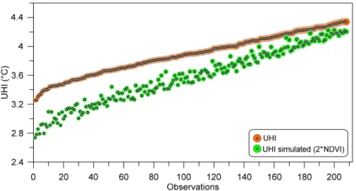
In the core area of the maximum heat island (Figure11), the intensity ranged from 3.2 to 4.3◦C. In the simulated UHI, however, the maximum and minimum values were lower (2.7–4.2◦C), with an average gain of approximately 0.1 to 0.5◦C. It was noted that the curve of the simulated UHI was always below that of the observed UHI, with minor differences occurring at higher intensities due to low NDVI values in points with a greater intensity (Figure12).
Atmosphere 2017, 8, 18 11 of 13
always below that of the observed UHI, with minor differences occurring at higher intensities due to low NDVI values in points with a greater intensity (Figure 12).
Figure 12. Maximum UHI and maximum simulated UHI with NDVI increased by 100%.
After a simulation of UHI with the NDVI increased by twice the simulated UHI, the area decreased by 45% (from 94,296 m2 to 51,931 m2).
4. Conclusions
The UHI in Iporá presents different spatial and time configurations in relation to big cities, with intensities tending towards lower values.
It is also noteworthy that:
1 The urban-geographical variables NDVI and UI were those that contributed the most to explain
the variability in the maximum UHI.
2 It was observed that the areas located in the valleys had lower thermal values, suggesting a cold air drainage as defined by Lopes [42].
3 During the occurrence of a maximum UHI, UHI > 1 °C classes had an area of approximately
15,000 km2, which corresponded to 90% of the urban area.
4 With the increase in NDVI, the UHI gradually decreased: the areas close to the Tamanduá stream
significantly decreased the values of UHI, or even presented a negative UHI (−4 °C, also known as cool islands), in simulations with NDVI increased by 80% and 100%.
5 In some areas of the city, there was little decrease in the intensity of UHIs due to little or no greening. Therefore, even with a 100% increase in NDVI, it would be too low and insufficient to significantly minimize UHIs.
6 The frequency of cool island classes increased with the increase in NDVI. The cool island class
−5 °C to −4 °C was only observed in the simulation with a 100% increase in NDVI. There was also a decrease in UHI classes 3–4 °C and 4–5 °C and an increase in low intensity classes due to the migration of more intense UHI to lower intensity classes.
7 With the increase in NDVI in the central area of a maximum UHI (dense urban area), there was
a perceptible and significant decrease in its intensity and size (a 45% area decrease).
As final conclusions, it is noteworthy that, by using multiple linear regression, it was possible to spatialize the UHI to the whole urban area, thereby providing an analysis of the urban setting from urban-geographical variables and thus performing prognostic simulations. Unger et al. [25], László and Szegedi [26], Bottyán and Unger [27], and Hart and Sailor [28] also concluded that a statistical type of modelling of the spatial distribution of maximum urban heat islands based on urban surface factors is an appropriate process because of the important roles it plays in increasing urban temperature. The relation between NDVI and biomass is a potentially useful way to determine how much vegetation planners need to plant to decrease 1 °C in city centers in order to properly address urban
UHI (°C)
Figure 12.Maximum UHI and maximum simulated UHI with NDVI increased by 100%.
After a simulation of UHI with the NDVI increased by twice the simulated UHI, the area decreased by 45% (from 94,296 m2to 51,931 m2).
4. Conclusions
The UHI in Iporá presents different spatial and time configurations in relation to big cities, with intensities tending towards lower values.
It is also noteworthy that:
1 The urban-geographical variables NDVI and UI were those that contributed the most to explain the variability in the maximum UHI.
2 It was observed that the areas located in the valleys had lower thermal values, suggesting a cold air drainage as defined by Lopes [42].
3 During the occurrence of a maximum UHI, UHI > 1◦C classes had an area of approximately 15,000 km2, which corresponded to 90% of the urban area.
4 With the increase in NDVI, the UHI gradually decreased: the areas close to the Tamanduá stream significantly decreased the values of UHI, or even presented a negative UHI (−4◦C, also known as cool islands), in simulations with NDVI increased by 80% and 100%.
5 In some areas of the city, there was little decrease in the intensity of UHIs due to little or no greening. Therefore, even with a 100% increase in NDVI, it would be too low and insufficient to significantly minimize UHIs.
6 The frequency of cool island classes increased with the increase in NDVI. The cool island class
−5◦C to−4◦C was only observed in the simulation with a 100% increase in NDVI. There was also a decrease in UHI classes 3–4◦C and 4–5◦C and an increase in low intensity classes due to the migration of more intense UHI to lower intensity classes.
7 With the increase in NDVI in the central area of a maximum UHI (dense urban area), there was a perceptible and significant decrease in its intensity and size (a 45% area decrease).
As final conclusions, it is noteworthy that, by using multiple linear regression, it was possible to spatialize the UHI to the whole urban area, thereby providing an analysis of the urban setting
from urban-geographical variables and thus performing prognostic simulations. Unger et al. [25], László and Szegedi [26], Bottyán and Unger [27], and Hart and Sailor [28] also concluded that a statistical type of modelling of the spatial distribution of maximum urban heat islands based on urban surface factors is an appropriate process because of the important roles it plays in increasing urban temperature.
The relation between NDVI and biomass is a potentially useful way to determine how much vegetation planners need to plant to decrease 1 ◦C in city centers in order to properly address urban climate changes. In the city center of Iporá, local planners may obtain a maximum gain of approximately 0.5◦C by doubling the vegetation on the streets. Future research must address the problem related to choosing the best plant species, taking into account that ventilation on streets should not be reduced by dense canopies in order to prevent higher concentrations of air pollution [29]. Acknowledgments:The authors would like to thank the São Paulo Research Foundation (FAPESP) for granting the scholarship (12/10450-0). They would also like to thank the anonymous reviewers and the editor for their helpful and constructive comments that greatly contributed towards improving the final version of this paper. Author Contributions:The manuscript was prepared by Elis Dener Lima Alves and revised by Antonio Lopes. All the authors reviewed the manuscript and contributed their part to improve the manuscript. All authors have read and approved the final manuscript.
Conflicts of Interest:The authors declare no conflict of interest.
References
1. Miao, S.; Chen, F.; LeMone, M.A.; Tewari, M.; Li, Q.; Wang, Y. An observational and modeling study of characteristics of urban heat island and boundary layer structures in Beijing. J. Appl. Meteorol. Climatol. 2009, 48, 484–501. [CrossRef]
2. Oke, T.R. City size and the urban heat island. Atmos. Environ. 1973, 7, 769–779. [CrossRef]
3. Arnfield, A.J. Two decades of urban climate research: A review of turbulence, exchanges of energy and water, and the urban heat island. Int. J. Climatol. 2003, 23, 1–26. [CrossRef]
4. Lopes, A.; Alves, E.; Alcoforado, M.J.; Machete, R. Lisbon urban heat island updated: New highlights about the relationships between thermal patterns and wind regimes. Adv. Meteorol. 2013, 2013, 487695. [CrossRef] 5. Chang, C.; Goh, K. The relationship between height to width ratios and the heat island intensity at 22:00 h
for Singapore. Int. J. Climatol. 1999, 19, 1011–1023.
6. Montávez, J.P.; Rodríguez, A.; Jiménez, J.I. A study of the urban heat island of Granada. Int. J. Climatol. 2000, 20, 899–911. [CrossRef]
7. Memon, R.A.; Leung, D.Y.C.; Liu, C.-H. An investigation of urban heat island intensity (UHII) as an indicator of urban heating. Atmos. Res. 2009, 94, 491–500. [CrossRef]
8. Ting, D.S.-K. Heat islands—Understanding and mitigating heat in urban areas. Int. J. Environ. Stud. 2012, 69, 1008–1011. [CrossRef]
9. Shashua-Bar, L.; Potchter, O.; Bitan, A.; Boltansky, D.; Yaakov, Y. Microclimate modelling of street tree species effects within the varied urban morphology in the Mediterranean city of Tel Aviv, Israel. Int. J. Climatol. 2010, 30, 44–57. [CrossRef]
10. Oke, T.R. Canyon geometry and the nocturnal urban heat island: Comparison of scale model and field observations. J. Climatol. 1981, 1, 237–254. [CrossRef]
11. Gartland, L. Ilhas de Calor: Como Mitigar Zonas de Calor em Áreas Urbanas; Oficina de textos: São Paulo, Brazil, 2010.
12. Sz ˝ucs, Á. Wind comfort in a public urban space—Case study within Dublin Docklands. Front. Archit. Res. 2013, 2, 50–66. [CrossRef]
13. Alcoforado, M.-J.; Andrade, H.; Lopes, A.; Vasconcelos, J.; Vieira, R. Observational studies on summer winds in Lisbon (Portugal) and their influence on daytime regional and urban thermal patterns. Merhavim 2006, 6, 90–112.
14. Grimmond, C.S.B.; King, T.S.; Cropley, F.D.; Nowak, D.J.; Souch, C. Local-scale fluxes of carbon dioxide in urban environments: Methodological challenges and results from Chicago. Environ. Pollut. 2002, 116, S243–S254. [CrossRef]
15. Oke, T.R. Boundary Layer Climates, 2nd ed.; Routledge: London, UK, 1987; pp. 1–435.
16. Georgescu, M.; Morefield, P.E.; Bierwagen, B.G.; Weaver, C.P. Urban adaptation can roll back warming of emerging megapolitan regions. Proc. Natl. Acad. Sci. USA 2014, 111, 2909–2914. [CrossRef] [PubMed] 17. Sharma, A.; Conry, P.; Fernando, H.J.S.; Hamlet, A.F.; Hellmann, J.J.; Chen, F. Green and cool roofs to mitigate
urban heat island effects in the Chicago metropolitan area: Evaluation with a regional climate model. Environ. Res. Lett. 2016, 11, 1–16. [CrossRef]
18. Coffee, J.E.; Parzen, J.; Wagstaff, M.; Lewis, R.S. Preparing for a changing climate: The Chicago climate action plan’s adaptation strategy. J. Great Lakes Res. 2010, 36 (Suppl. 2), 115–117. [CrossRef]
19. Alcoforado, M.-J.; Andrade, H. Nocturnal urban heat island in Lisbon (Portugal): Main features and modelling attempts. Theor. Appl. Climatol. 2006, 84, 151–159. [CrossRef]
20. Charabi, Y.; Bakhit, A. Assessment of the canopy urban heat island of a coastal arid tropical city: The case of Muscat, Oman. Atmos. Res. 2011, 101, 215–227. [CrossRef]
21. Brandsma, T.; Wolters, D. Measurement and statistical modeling of the urban heat island of the city of Utrecht (the Netherlands). J. Appl. Meteorol. Climatol. 2012, 51, 1046–1060. [CrossRef]
22. Mihalakakou, G.; Flocas, H.A.; Santamouris, M.; Helmis, C.G. Application of Neural networks to the simulation of the heat island over Athens, Greece, using synoptic types as a predictor. J. Appl. Meteorol. 2002, 41, 519–527. [CrossRef]
23. Saitoh, T.S.; Shimada, T.; Hoshi, H. Modeling and simulation of the Tokyo urban heat island. Atmos. Environ. 1996, 30, 3431–3442. [CrossRef]
24. Stewart, I.D.; Oke, T.R.; Krayenhoff, E.S. Evaluation of the ‘local climate zone’ scheme using temperature observations and model simulations. Int. J. Climatol. 2014, 34, 1062–1080. [CrossRef]
25. Unger, J.; Bottyán, Z.; Gulyás, A.; Kevei-Bárány, I. Urban temperature excess as a function of urban parameters in szeged, part 2: Statistical model equations. Acta Climatol. Chorol. 2001, 34–35, 15–21. 26. László, E.; Szegedi, S. A multivariate linear regression model of mean maximum urban heat island: A case
study of Beregszász (Berehove), Ukraine. Q. J. Hungarian Meteorol. Serv. 2015, 119, 409–423.
27. Bottyán, Z.; Unger, J. A multiple linear statistical model for estimating the mean maximum urban heat island. Theor. Appl. Climatol. 2003, 75, 233–243. [CrossRef]
28. Hart, M.A.; Sailor, D.J. Quantifying the influence of land-use and surface characteristics on spatial variability in the urban heat island. Theor. Appl. Climatol. 2008, 95, 397–406. [CrossRef]
29. Alcoforado, M.-J.; Andrade, H.; Lopes, A.; Vasconcelos, J. Application of climatic guidelines to urban planning. Landsc. Urban Plan. 2009, 90, 56–65. [CrossRef]
30. IBGE, Cidades. 2015. Available online: http://www.cidades.ibge.gov.br/ (accessed on 1 September 2016). 31. Oke, T.R. Initial Guidance to Obtain Representative Meteorological Observations at Urban Sites; IOM Report No.
81, WMO/TD. No. 1250; World Meteorological Organization (WMO): Geneva, Switzerland, 2006.
32. Martin-Vide, J.; Sarricolea, P.; Moreno-García, M.C. On the definition of urban heat island intensity: The ‘rural’ reference. Front. Earth Sci. 2015, 3, 1–6. [CrossRef]
33. Alves, E. Seasonal and spatial variation of surface urban heat island intensity in a small urban agglomerate in Brazil. Climate 2016, 4, 61. [CrossRef]
34. Kawamura, M.; Jayamana, S.; Tsujiko, Y. Relation between social and environmental conditions in Colombo Sri Lanka and the urban index estimated by satellite remote sensing data. Int. Arch. Photogramm. Remote Sens. 1996, XXXI, 321–326.
35. As-syakur, A.R.; Adnyana, I.W.S.; Arthana, I.W.; Nuarsa, I.W. Enhanced built-up and bareness index (EBBI) for mapping built-up and bare land in an urban area. Remote Sens. 2012, 4, 2957–2970. [CrossRef]
36. Lapponi, J.C. Estatistica Usando Excel, 4th ed.; CAMPUS—RJ: Rio de Janeiro, Brazil, 2005.
37. Gál, T.; Balázs, B.; Geiger, J. Modelling the maximum development of urban heat island with the application of gis based surface parameters in szeged (part 2): Stratified sampling and the statistical model. Acta Climatol. Chorol. 2005, 38–39, 59–69.
38. Unger, J. Modelling of the annual mean maximum urban heat island using 2D and 3D surface parameters. Clim. Res. 2006, 30, 215–226. [CrossRef]
39. Montgomery, D.C.; Peck, E.A.; Vining, G.G. Introduction to Linear Regression Analysis, 5th ed.; John Wiley & Sons: New York, NY, USA, 2012.
41. Hu, Y.; Su, C.; Zhang, Y. Research on the microclimate characteristics and cold island effect over a reservoir in the Hexi Region. Adv. Atmos. Sci. 1988, 5, 117–126. [CrossRef]
42. Lopes, A. Drenagem e acumulação de ar frio em noites de arrefecimento radiativo. Um exemplo no vale de Barcarena (Oeiras). Finisterra 1995, 30, 149–164. [CrossRef]
43. Trancoso, R.; Sano, E.E.; Meneses, P.R. The spectral changes of deforestation in the Brazilian tropical savanna. Environ. Monit. Assess. 2015, 187, 4145. [CrossRef] [PubMed]
44. Liu, W.; Ji, C.; Jiang, X.; Zhong, J. Relationship between NDVI and the urban heat island effect in Beijing area of China. Proc. SPIE Int. Soc. Opt. Eng. 2005, 5884, 58841R.
45. Mackey, C.W.; Lee, X.; Smith, R.B. Remotely sensing the cooling effects of city scale efforts to reduce urban heat island. Build. Environ. 2012, 49, 348–358. [CrossRef]
© 2017 by the authors; licensee MDPI, Basel, Switzerland. This article is an open access article distributed under the terms and conditions of the Creative Commons Attribution (CC-BY) license (http://creativecommons.org/licenses/by/4.0/).