Resilience: statistical study of psychosocial and biological predictors at the workplace

2019

UNIVERSIDADE DE LISBOA

FACULDADE DE CIÊNCIAS

DEPARTAMENTO DE ESTATÍSTICA E INVESTIGAÇÃO OPERACIONAL

Resilience: statistical study of psychosocial and biological

predictors at the workplace

Heloísa Gabriela de Castro Vasconcelos Gonçalves Galante

Mestrado em Bioestatística

Trabalho de Projeto orientado por:

Professora Doutora Lisete Sousa

i

Acknowledgments

Às minhas orientadoras, Professora Lisete e Doutora Maria João, pelo enorme apoio dado durante todo o processo deste projeto.

Aos meus pais, Luísa e Marc, e irmã Gabriela, que me acompanharam ao longo destes meses e sempre me compreenderam.

Aos meus avós, Fátima e Herculano, e Tia Nini, que me motivaram a ser forte e nunca desistir.

À minha Tia São, que não chegou a assistir ao final desta etapa, mas que decerto me vê.

Ao meu melhor amigo Bruno, que sempre soube como me sentia.

iii

Resumo

A resiliência pode ser definida como a capacidade de um indivíduo adaptar-se com facilidade a infortúnios ou mudanças inesperadas. Também é vista como um mecanismo positivo de resposta a acontecimentos stressantes, desde desastres naturais a questões financeiras, problemas de saúde, divórcio e morte. A resiliência é estudada desde o século XIX e desde aí demonstra uma evolução conceptual, tendo sido concebida como trajetória, contínuo, sistema, característica, processo, ciclo e categoria qualitativa. Nas teorias que consideram a resiliência uma característica, acredita-se que uma combinação de outras características físicas e psicológicas potenciem a capacidade de ser resiliente. Perante a cultura do trabalho que se verifica no mundo contemporâneo, é interessante estudar o papel da resiliência em trabalhadores, cujo maior fator de stress é o trabalho em si e todas as suas componentes e ligações com as restantes áreas da vida pessoal, de modo a entender de que forma estes diversos fatores podem influenciar os seus níveis de resiliência.

O principal objetivo deste estudo é identificar possíveis preditores de resiliência em trabalhadores. Com este intuito, os 1385 colaboradores de uma instituição bancária que cumpriam os critérios de inclusão pré-definidos foram convidados a participar no projeto. Aos 260 que aceitaram fazer parte do estudo e realizar exames laboratoriais, foi aplicado um questionário pormenorizado acerca do respondente, do seu trabalho, experiências e vida pessoal, incluindo diversos tipos de variáveis (sociodemográficas, relacionadas com o trabalho, relacionadas com o estilo de vida, clínicas), para além de diversas escalas validadas referentes a estes temas (ASSET, MHI-5, Escala de Satisfação no Trabalho, CAGE, Escala de Felicidade Subjetiva, OSLO, Presentismo e Absentismo). A isto, juntam-se as variáveis bioquímicas provenientes dos resultados das análises laboratoriais. A variável resiliência foi medida através das versões de 25 e 10 itens da Escala de Resiliência de Connor-Davidson. Estes dados foram recolhidos entre Novembro de 2012 e Junho de 2013. A base de dados contendo todas as variáveis foi corrigida e validada no contexto deste projeto antes de se iniciar o processo de análise abaixo descrito.

Primeiramente, foi realizada uma análise exploratória dos dados, de modo a caracterizar os respondentes. Seguidamente, decidiu-se qual das versões da escala de resiliência seria considerada a medida única de resiliência durante o decorrer da análise, através do cálculo do coeficiente de correlação ordinal de Spearman e do respetivo teste de significância. Os resultados demonstram que o valor desta medida sugere uma associação elevada entre ambas as versões, o que significa que a menos redundante, de 10 itens, deve ser escolhida. Depois, devido ao grande número de possíveis preditores na base de dados, procedeu-se a uma pré-seleção das variáveis cuja associação com a resiliência (se numéricas, usando o coeficiente de correlação de Spearman) ou diferença entre grupos relativamente à resiliência (se categóricas, usando os testes de Mann-Whitney ou Kruskal-Wallis) fossem estatisticamente significativas. As variáveis pré-selecionadas foram integradas num modelo de regressão inicial, ao qual se aplicou a seleção stepwise de modo a obter-se um modelo mais parcimonioso que simultaneamente explicasse a maior percentagem possível da variabilidade da resiliência. Este modelo final, validado no que diz respeito aos pressupostos de uma análise de regressão, engloba como preditores a saúde mental, segurança no trabalho e sobrecarga laboral (medidos por subescalas do ASSET), ter interesses ou hobbies, tomar medicação para a ansiedade crónica e o nível de presentismo, e explica aproximadamente 35% da variabilidade da resiliência. Possíveis interações a adicionar a este modelo final foram analisadas relativamente aos preditores descritos, mas não se demonstraram estatisticamente significativas na análise de regressão. Por último, com o objetivo de entender de melhor forma a estrutura das variáveis

iv

selecionadas inicialmente, foi aplicada uma análise fatorial múltipla de dados mistos. Esta metodologia inovadora propõe alargar o conceito da análise fatorial múltipla, em que existem vários grupos de variáveis mas em que cada grupo contém apenas variáveis do mesmo tipo, para os casos em que estes grupos acomodam tanto variáveis do tipo numérico como categórico. Os grupos formados com as variáveis em questão foram “Trabalho” e “Saúde Física e Mental”. As três primeiras componentes principais explicam pouco mais de 20% da variabilidade dos dados. Relativamente à primeira componente principal, o impacto de ambos os grupos é quase idêntico. O grupo "Trabalho" contribui mais para a segunda componente principal, enquanto que para a terceira o grupo "Saúde Física e Mental" apresenta a maior contribuição, embora a diferença seja bastante pequena.

As limitações deste estudo prendem-se essencialmente com a pequena dimensão da amostra, com o facto de não ter sido recolhida aleatoriamente e por ser proveniente de um tipo muito limitado de trabalhadores, o que pode enviesar os resultados. Não obstante, a análise realizada foi capaz de dar resposta aos objetivos do projeto e revela-se importante e relevante para um maior conhecimento do fenómeno da resiliência e da sua importância nos trabalhadores. Futuros estudos com amostras de maior dimensão e mais variabilidade de trabalhadores podem consolidar e confirmar os resultados obtidos, aprofundando esta temática.

Palavras-chave: resiliência, dados categóricos, métodos não-paramétricos, regressão múltipla, análise

v

Abstract

Resilience is one of the most important characteristics of an employee in the workaholic culture of our current society. The main purpose of this study is to discover which other traits, habits and features can significantly influence and impact resilience levels. For this purpose, a comprehensive questionnaire was applied to 260 workers from a banking institution between November 2012 and June 2013, including sociodemographic, work-related, lifestyle-related, clinical and biochemical variables, while also comprising several validated scales. Resilience was measured with the 25-item and 10-item versions of the Connor-Davidson Resilience Scale. After a pre-selection of the survey’s variables with a statistically significant association (if numerical) or difference between groups (if categorical) regarding resilience, its best predictors were identified through a regression analysis: ASSET’s Psychological wellbeing, Job security and Overload scales, having interests/hobbies, taking medication for chronic anxiety and the percentage of work performance loss (presenteeism). This regression model explains about 35% of resilience’s variability. Also, in an attempt to understand the structure of the resilience predictors and reduce its dimension, a multiple factor analysis of mixed data was conducted regarding the pre-selected variables, which were divided in two conceptual groups: “Work” and “Physical and Mental Health”. The first three principal components explain about 20% of their variability. This study was important to provide more evidence and information regarding resilience predictors at the workplace and exploring the relationships between resilience and several scales, some of which have not been analyzed by the scientific community so far. However, further studies with larger sample sizes, mixed categories of workers and other types of variables are needed to confirm the obtained results. This knowledge can lead to improvements in workers’ resilience levels, and therefore increase productivity and work satisfaction of a company’s employees, which is fruitful to both.

Keywords: resilience, categorical data, non-parametric methods, multiple regression, multiple factor

vii

Table of contents

1.5 Study Design and Description ...3

2. Statistical Methodology. ...9

2.1 Spearman rank correlation coefficient ...9

2.2 One-way analysis of variance ...11

2.3 Mann-Whitney U test ...12

2.4 Kruskal Wallis test ...13

2.5 Conover post-hoc test ...14

2.6 Benjamini-Hochberg correction ...14

2.7 Multiple Linear Regression ...15

2.8 Fisher’s exact test ...20

viii

3. Results. ...23

3.1 Exploratory analysis ...23

3.2 Choosing the dependent variable ...27

3.3 Choosing the independent variables ...27

3.4 Resilience prediction ...40

3.5 Multiple Factor Analysis of Mixed Data ...47

Discussion. ...53

References. ...57

Appendices. ...61

A. List of variables ...61

ix

List of tables

Table 2.1.1: Interpretation of Spearman's coefficient according to Fowler, Cohen and Jarvis (2009). .10

Table 2.2.1: ANOVA components. ...11

Table 2.7.1: ANOVA components for multiple regression analysis. ...16

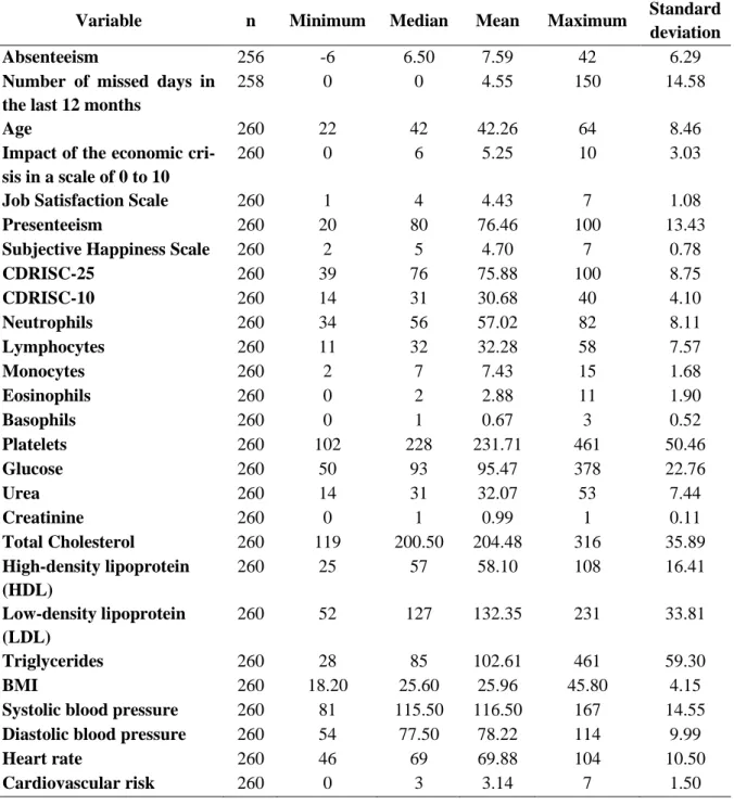
Table 3.1.1: Summary of some of the questionnaire’s numerical variables. ...24

Table 3.1.2: Summary of some of the questionnaire’s categorical variables. ...25

Table 3.3.1.1: Spearman’s correlation coefficient estimates and the corrected p-values for the respec-tive significant tests. ...28

Table 3.3.2.1: Mann-Whitney and Kruskal-Wallis tests’ corrected p-values. ...29

Table 3.4.1: Parameter estimates and their standard errors, observed values of the t-statistic and p-val-ues for Model 1. ...40

Table 3.4.2: Stepwise selection’s final models. ...42

Table 3.4.3: Parameter estimates and their standard errors, observed values of the t-statistic and p-val-ues for Model 1.2. ...42

Table 3.4.4: VIFs of the independent variables of Model 1.2. ...45

Table 3.5.1: Groups of variables and their types for the implementation of MFA of mixed data...47

Table 3.5.2: Eigenvalues, percentage of explained variance and cumulative percentage of explained variance for the first ten principal components of the MFA for mixed data. ...47

Table 3.5.3: Eigenvalues of each variable group for the first three principal components. ...48

Table 3.5.4: Percentage of explained variance of each variable for the first three principal compo-nents. ...48

Table 3.5.5: Squared loadings of each variable for the first three principal components. ...49

xi

List of figures

Figure 1.1.1: Resilience model (George Mason University's Resilience Model, n.d.) ...1

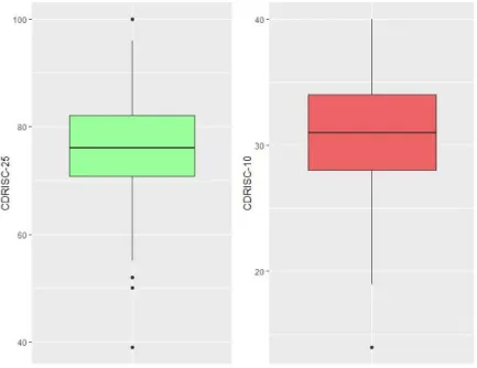
Figure 3.1.1: Boxplots of CDRISC-25 (left) and CDRISC-10 (right). ...23

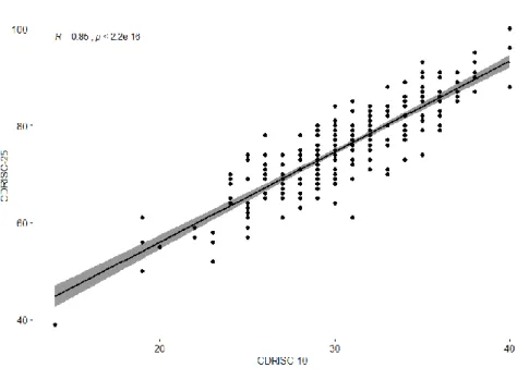
Figure 3.2.1: Scatter plot of CDRISC-10 vs CDRISC-25. ...27

Figure 3.3.1.1: Scatter plots of CDRISC-10 vs the variables with significant Spearman’s rank correla-tion coefficient. ...28

Figure 3.3.2.1: Parallel boxplots of CDRISC-10 vs the variables with significant Mann-Whitney’s test. ...30

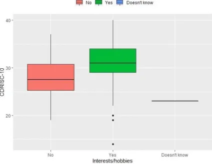
Figure 3.3.2.1.1: Parallel boxplots of CDRISC-10 vs Interests/hobbies. ...31

Figure 3.3.2.1.2: Parallel boxplots of CDRISC-10 vs Work relationships. ...31

Figure 3.3.2.1.3: Parallel boxplots of CDRISC-10 vs Overload. ...32

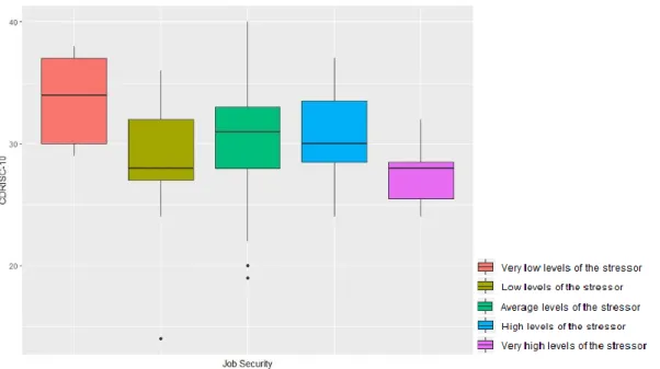
Figure 3.3.2.1.4: Parallel boxplots of CDRISC-10 vs Job security. ...33

Figure 3.3.2.1.5: Parallel boxplots of CDRISC-10 vs Control. ...33

Figure 3.3.2.1.6: Parallel boxplots of CDRISC-10 vs Resources and communication. ...34

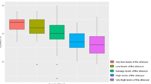
Figure 3.3.2.1.7: Parallel boxplots of CDRISC-10 vs Aspects of the job. ...35

Figure 3.3.2.1.8: Parallel boxplots of CDRISC-10 vs Perceived commitment of employee to organiza-tion. ...35

Figure 3.3.2.1.9: Parallel boxplots of CDRISC-10 vs Physical health. ...36

Figure 3.3.2.1.10: Parallel boxplots of CDRISC-10 vs Psychological wellbeing. ...37

Figure 3.3.2.1.11: Parallel boxplots of CDRISC-10 vs Productivity...37

Figure 3.3.2.1.12: Parallel boxplots of CDRISC-10 vs Depression. ...38

Figure 3.3.2.1.13: Parallel boxplots of CDRISC-10 vs Chronic anxiety. ...39

Figure 3.3.2.1.14: Parallel boxplots of CDRISC-10 vs Medication for chronic anxiety. ...39

Figure 3.4.1: Histogram (left) and boxplot (right) of Model 1.2’s residuals. ...43

Figure 3.4.2: Quantile-quantile plot of Model 1.2’s residuals. ...44

Figure 3.4.3: Scatter plot of predicted values vs residuals of Model 1.2. ...44

Figure 3.4.4: Cook’s distances for Model 1.2. ...46

Figure 3.5.1: Correlation circles of the numerical variables for the combinations of the first three prin-cipal components. ...50

Figure 3.5.2: Contribution of each variable for the combinations of the first three principal compo-nents. ...51

Figure 3.5.3: Contribution of each group for the combinations of the first three principal components. ...52

1

Chapter 1

Introduction

1.1 Definition

Resilience can be defined as the capability to adapt with ease to misfortune or unexpected change (Merriam-Webster, 2019). It is a coping mechanism or response to stressful experiences, that can be related to any type of problem or challenge, ranging from natural disasters to financial issues, health concerns, divorce and death.

The concept of resilience has been studied since the 1800s and is continuously evolving. During its development, resilience has been constructed as a trajectory, a continuum, a system, a trait, a process, a cycle and a qualitative category (Jackson et al., 2007). In theories that consider resilience a trait, it is believed that a combination of physical and psychological characteristics, including body chemistry and personality factors, gives individuals the skills to be resilient (Jacelon, 1997).

Resilient people tend to not become as bothered, upset or fearful when adversities happen as people with less resilience do, although that does not mean they do not feel them as deeply. Having resilience merely implies that the subject of a certain unpleasant event utilizes their skills, strengths and knowledge to overcome it and grow from it, without losing hope or falling into despair. Figure 1.1.1 provides an illustration of the most common characteristics and states conceptually associated to resilience.

2

1.2 Literature review

Resilience at the workplace

According to the World Health Organization (1994), the majority of the world’s population (58%) spends one-third of their adult life at work. This allows the achievement of material and economic goals and provides a better quality of life. However, there are several jobs in many countries that still entail hazards to health, therefore reducing the well-being, working capacity and life span of working individuals.

In a workplace setting, various demanding situations can take place: heavy workload, impractical deadlines, poor communication, rigid schedules, competition between colleagues, discrimination and general bad work environment. These can lead to workers’ discouragement, lack of motivation and mental and physical health problems. To deal with this constant pressure and stress, resilience is a needed and valuable skill. It has been associated with various positive states, including optimism, zest, curiosity, energy and openness to experience (Tugade & Fredrickson, 2004), which can boost performance and creativity.

Work-related psychosocial risk factors or stressors are likely to have an impact in physical and mental health through closely interrelated emotional, cognitive, behavioral and physiological mechanisms. Strong evidence was found that high job demands, low job control, low co-worker support, low supervisor support, low procedural and relational justice and a high effort–reward imbalance predict the incidence of stress-related mental disorders, for which resilience can be a structural protective factor (Rutter, 2006).

Environmental, demographic and lifestyle factors

Tugade and Fredrickson (2004) suggest that the ability to find positive meaning in adverse situations and to regulate negative emotions contributes to personal resilience. Studies have shown a link between low resilience and several mental health outcomes, such as burnout, secondary traumatic stress, depression and anxiety (Rees et al., 2015). Furthermore, evidence on resilient survivors of violent trauma shows that these exhibited better health and less severe post-traumatic stress disorder symptoms than those who were not resilient (Connor, Davidson & Lee, 2003).

Characteristics like sex, education level, income level and history of childhood abuse are thought to contribute to the prediction of resilience: females, individuals with lower levels of education and income and individuals with history of childhood trauma report diminished resilience (Sparks et al., 1997). Other factors such as age, race/ethnicity, substance use, social support, chronic diseases, recent life stressors and past traumatic events are also shown to impact individuals’ level of resilience (Bonanno et al, 2007). However, some studies claim there is no relationship between resilience and social support and lifestyle or work-related factors (Corina & Adriana, 2013; Black et al., 2017), although it is generally acknowledged that resilience moderates various stress types (Liu et al., 2018).

As far as individual personality traits go, a negative correlation between resilience and neuroticism and positive associations with extraversion and conscientiousness have been accounted for (Fayombo, 2010). Bonanno et al. (2002) discusses hardiness, self-enhancement, repressive coping, positive emotions and laughter as being resilience-promoting.

3

1.3 Research objectives

The general objective of this study is the identification of sociodemographic, psychological, clinical and biological factors that impact workers’ resilience and global mental health. This study aims to answer the following questions:

1. What factors impact the resilience level at the workplace? 2. Is there an underlying structure to the main resilience predictors?

1.4 Project outline

This project begins with the introduction above, stating the study’s subject, the state of the art and reasons for its importance and relevance in today’s society, followed by a thorough description of the dataset. Next, a methodology chapter describes the theoretical principals behind the statistical methods used. This is followed by the results chapter, where the outcomes of the statistical analyses are presented and compared. It ends with a discussion chapter, where the obtained results are critically examined and further work and research regarding this subject are suggested.

1.5 Study Design and Description

The study presented in this project is descriptive, with a cross sectional design. It was conducted in the context of the project “Health Impact Assessment of Employment Strategies”, led by Doctor Maria João Heitor dos Santos in 2011, resulting of a collaboration protocol between the then High Commissioner of Health, the Institute of Preventive Medicine and Public Health of the Faculty of Medicine of the University of Lisbon and the National Institute of Health Doutor Ricardo Jorge. It contains data from a survey applied to employees of Caixa Económica Montepio Geral (CEMG) in the Lisbon County, between November 2012 and June 2013. The questionnaire itself is not included in the Appendices section due to it being confidential.

1.5.1 Sample

Eligible subjects for the study were identified from the employee population of CEMG using the following selection criteria:

• Employees between the age of 18 and 69 years;

• Employees able to understand and sign an informed consent.

A total of 1385 Lisbon County’s CEMG employees were identified in these conditions. All were sent an invitation to participate in the survey through their institutional email, and only those who voluntarily wanted to take part in the project were included in the study. Therefore, the resulting sample is non-random.

From the 1385 invited employees, 405 responded to the survey. A blood sample and anthropometric measures were also collected from 260 participants out of the 405. Matching of participants between the survey and blood samples was possible using an ID linked to a name and email address, to guarantee confidentiality.

4

In order to include the variables collected from the blood sample and biochemical parameters in this study, only the data from the 260 participants was used in the analysis.

1.5.2 Description of the variables

From the original dataset, containing 406 raw variables, a subset of 106 variables indicated by the project leader was considered for this analysis. This set contains variables which are reported by experts and literature as being of interest regarding the study of the resilience phenomenon.

The final dataset contains the following types of variables (detailed in Appendix A): • Sociodemographic • Work-related • Lifestyle-related • Clinical • Biochemical • Scales

- CDRISC Scale (Connor & Davidson, 2003), a brief self-rated assessment to quantify individual

resilience. The CDRISC is composed of 25 items, each rated on a 5-point scale of responses (0– 4). The scale is rated based on how the subject felt over the previous month. The total score ranges from 0–100, with higher scores reflecting greater resilience;

- ASSET (Cooper, Sloan & Williams, 1988), a short stress evaluation tool to assess the risk of

workplace stress, containing twelve subscales: eight of which evaluate the workers’ job per-ception, two of which evaluate their attitude towards the organization and the other two which evaluate their physical and mental health;

- Mental Health Index Scale - MHI-5 (Veit & Ware, 1983; Ribeiro, 2001), a scale of 5 items,

each rated in a 6-point scale, used for the measurement of mental health status;

- Oslo Social Support Scale (Dalgard, 1996; Dalgard et al. 2006), a scale of 3 items, two of them

rated in a 5-point scale and one rated in a 4-point scale, that allows overall assessment of social support;

- Subjective Happiness Scale (Lyubomirsky & Lepper, 1999), a scale of 4 items, each rated in

a 7-point scale, which evaluates one’s self-assessment of subjective happiness;

- CAGE Scale (Ewing, 1984), a scale of 4 items, each rated as 0 (if the answer is “No”) or 1 (if

the answer is “Yes”), to measure alcohol consumption;

- Job Satisfaction Scale (Cooper, Sloan & Williams, 1988), a scale of 7 items, each rated in a

7-point scale, that evaluates one’s level of satisfaction with their job;

- Presenteeism Scale (Kessler et al. 2004; 2003), a scale of 3 items, each ranging from 0 to 10,

5

1.5.3 Data preparation

• Database cleaning

Prior to the analysis itself, an internal data cleaning was conducted, in order to identify inaccu-rate or incorrect records and proceed to their correction or removal, to assure the consistency of the database.

• New variables

Based on the objectives of this project, a set of extra indicators was computed from some of the original variables in the dataset:

- CDRISC-10: A new variable for resilience was created, using the 10 item version of the

CDRISC. This version is obtained from the 25 item, based on a psychometric analysis that al-lowed the identification of the 10 items that best captured the features of resilience with minimal redundancy. The 10 item version (final scores range from 0 to 40) comprises items 1, 4, 6, 7, 8, 11, 14, 16, 17, 19 from the original scale.

- Absenteeism: Absenteeism refers to the usual pattern of absence in a function or obligation

(Weiner, Schmitt & Highhouse, 2012). To create an absenteeism indicator, the difference be-tween the number of effective work hours and the number of expected work hours was com-puted. Thus, negative values represent loss in work hours, positive values represent surpluses in work hours and 0 represents absence of loss (or surplus) of work hours.

- Cardiac Risk Index: This indicator is based on the standards of the Portuguese Society of

Car-diology, according to which its risk factors are:

Modifiable factors: Smoking;

High blood pressure (pre-hypertensive and hypertensive); Diabetes; Obesity; High cholesterol; Sedentarism; Psychosocial stress. Non-modifiable factors: Male gender;

Age greater than 55 years; Heredity.

6

For each risk factor present in an individual a value of 1 was considered, except for heredity because no information was available. A cardiac risk indicator was computed through the sum of the values for the set of risk factors. Therefore, the values of this indicator range from 0 to 9, and the higher the value, the greater the cardiovascular risk.

Besides the variables above, there was also the need to work with the total score for each scale comprised in the survey, instead of the individual questions’ scores. For this purpose, the following scale scores were calculated:

- ASSET subscales: First, each of the subscales’ sten score (Colman, 2019) was computed using

the individual level norms for the general population group, according to the ASSET Norm Supplement. Then, to obtain final scores, the following rules were applied to the “perceptions of your job”, “attitudes to your organization” and “your health” scales, respectively:

Scores below sten 3 indicate very low levels of the stressor/ very low levels of commit-ment/ very good health levels (coded as 1);

Scores below sten 4 indicate low levels of the stressor/ low levels of commitment/ good health levels (coded as 2);

Scores within the range defined by sten 4 to sten 7 indicate average levels of the stressor, commitment and health (coded as 3);

Scores above sten 7 indicate high levels of the stressor/ high levels of commitment/ poor health levels (coded as 4);

Scores above the sten 8 indicate very high levels of the stressor/ very high levels of commitment/ very poor health levels (coded as 5).

- MHI-5: The questions “How much of the time in the previous 4 weeks have you felt calm and

peaceful?” and “How much of the time in the previous 4 weeks have you been a happy person?” are reversed (a 6 turned into a 1, a 5 into a 2, a 4 into a 3, a 3 into a 4, a 2 into a 5 and a 1 into a 6). Then, the mean of the 5 items is multiplied by 100 and divided by 5, varying from 0-100. Individuals with a score lower or equal to 52 present psychological distress;

- OSLO-3: A sum index was computed using the raw individual scores of the 3 questions,

rang-ing from 3 to 14. A score of 3-8 means “poor support”, 9-11 means “moderate support” and 12-14 means “strong support”;

- Subjective Happiness Scale: To score the scale, the question “Some people are generally not

very happy. Although they are not depressed, they never seem as happy as they might be. To what extent does this characterization describe you?” was reversed (a 7 turned into a 1, a 6 into a 2, a 5 into a 3, a 3 into a 5, a 2 into a 6 and a 1 into a 7), and the mean of the 4 items was calculated;

- CAGE: The final score corresponds to the sum of the 4 items. A sum greater than or equal to 2

indicates a high probability of alcohol dependence;

- Job Satisfaction Scale: An overall indicator was obtained by calculating the arithmetic mean

of the seven items;

- Presenteeism Scale: Absolute Presentism corresponds to the proportion of the loss of one's

performance at work, calculated by multiplying by 10 the response to the question “On a 0-to-10 scale, how would you rate your overall job performance on the days you worked during the

7

past 4 weeks (28 days)?”. This indicator varies between 0 and 100, and the higher its value, the lower the performance loss.

1.5.4 Software

The database preparation and statistical analysis were conducted using Microsoft Excel and R Studio (R Core Team, 2019), respectively.

1.5.5 Ethical considerations

This study was approved by two institutional ethical committees: the Ethics Committee for Health of the National Institute of Health Doutor Ricardo Jorge (INSA) and the Ethics Committee for Health of the Lisbon/North Hospital Center of the Faculty of Medicine of the University of Lisbon (CHLN/FMUL). It was also approved by the National Commission of Data Protection (CNPD). All participants signed an informed consent.

1.5.6 Previous studies in the context of the project

The data corresponding to the 405 questionnaire respondents has been initially studied, in the context of the original project. The CDRISC scale was validated for a Portuguese sample (Faria Anjos et al., 2019), where the three identified dimensions of resilience were the self-efficacy, spirituality and social support factors present in the scale. The Portuguese version of ASSET was validated in terms of its psychometric properties and its convergent validity was tested (Heitor et al., 2018).

9

Chapter 2

Statistical Methodology

This project is based on workers’ responses to a comprehensive questionnaire regarding several dimensions of their life. Survey variables are mostly categorical, which can be limiting as far as statistical methodology goes – most studies with a similar background stick to scale validations and contingency table analyses. In this study, the methods were chosen taking into account its research questions and the quality of the data.

Firstly, as there are two measures for resilience, the Spearman rank correlation coefficient was calculated with the purpose of selecting which should be considered the most adequate dependent variable for a future regression model. This method was also used to select the relevant numerical independent variables regarding resilience and to check for potential associations between them. Concerning the categorical independent variables, Mann-Whitney (for variables with only two groups) and Kruskal-Wallis (for variables with more than two groups) tests were applied to check for significant differences in resilience between groups. For the Kruskal-Wallis tests with a significant p-value, Conover’s test was used in order to identify which of the respective variables’ groups present statistically significant differences in resilience levels. Throughout these analyses, the Benjamini-Hochberg correction was applied to correct p-values in cases of multiple testing. A multiple regression analysis was conducted to study the linear relationship between resilience and the selected predictor candidates. To check for plausible interaction terms to add to this regression model, Fisher’s exact test was applied to determine if there was a statistically significant association between any two pairs of categorical variables present in the final multiple regression model. The methodologies described so far mean to answer the first research objective formulated in Section 1.3. Finally, a multiple factor analysis of mixed data was conducted to reduce dimensionality and explore the structure of the initially selected variables, considering the presence of both categorical and numerical variables and their potential to form conceptual groups. This method aims to answer the second research objective mentioned in Section 1.3. The R functions and respective packages that allowed the implementation of these techniques are mentioned throughout the text. The significance level 𝛼 = 0.05 was used for all methods. Also, it should be mentioned that the Levene and Shapiro-Wilk tests for the validation of the ANOVA and linear regression assumptions are not detailed in this chapter because they are widely known and not the main focus of the present statistical analysis.

2.1 Spearman rank correlation coefficient

The Spearman rank correlation coefficient (𝑟𝑠) represents a non-parametric alternative to the Pearson

product-moment correlation. This measure can be applied to numerical or ordinal variables and is robust when extreme values are present. If there is an intention to perform hypotheses tests over the population’s correlation coefficient, Spearman’s coefficient can also substitute Pearson’s coefficient

10

when the latter’s assumptions of bivariate normality or linearity are not verified by the data (Hauke & Kossowski, 2011).

Spearman’s rank correlation coefficient assesses how well an arbitrary monotonic function can describe a relationship between two variables without making assumptions about their probability distributions. It can range from -1 to +1, where a value of 0 indicates that there is no linear association between ranks, and, therefore, no monotonic relationship between the variables, a value of -1 indicates a perfect negative correlation between ranks and a value of +1 represents a perfect positive correlation between ranks (Table 2.1.1).

Table 2.1.1: Interpretation of Spearman's coefficient according to Fowler, Cohen and Jarvis (2009).

|𝒓_𝒔| Association strength 0.90 – 1.00 Perfect 0.70 – 0.89 Strong 0.40 – 0.69 Moderate 0.20 – 0.39 Weak 0.00 – 0.19 Very weak

Let there be 𝑋 and 𝑌, a pair of random variables. For a sample of size 𝑛, the 𝑛 raw scores 𝑥𝑖, 𝑦𝑖, 𝑖 =

1, … , 𝑛, are converted to ranks. The formula for

𝑟

𝑟

= 1 −

𝑛(𝑛2₋₁₎ (2. 1)

where 𝑟𝑥𝑖 is the rank of 𝑥𝑖, 𝑟𝑦𝑖 is the rank of 𝑦𝑖 and 𝑑𝑖 = 𝑟𝑥𝑖− 𝑟𝑦𝑖.

The formula to use when there are tied ranks is:

𝑟

=

∑ ( 𝑟𝑖 _𝑥𝑖−𝑟̅ )(𝑟𝑥 _𝑦𝑖−𝑟̅ )𝑦

√∑ ( 𝑟𝑖 𝑥𝑖−𝑟̅ )𝑥2(𝑟_𝑦𝑖−𝑟̅ )𝑦 2

(2. 2)

To test whether the Spearman correlation coefficient is significantly different from zero, the following is hypothesized:

H0: There is no association between 𝑋 and 𝑌; H1: There is an association between 𝑋 and 𝑌.

For a large number of (𝑋𝑖, 𝑌𝑖) pairs, the distribution of 𝑇 = 𝑅𝑠√ 𝑛−2

1−𝑅𝑠2 can be approximated by a

Student’s t distribution with 𝑛 − 2 degrees of freedom, under the null hypothesis. For a significance level of 𝛼, the null hypothesis is rejected if the observed value of the test statistic |𝑇0| ≥ 𝑡(𝑛−2, 1−𝛼 2⁄ ),

which represents the 1 − 𝛼 2⁄ quantile of a Student’s t distribution with 𝑛 − 2 degrees of freedom.

11

2.2 One-way analysis of variance

The one-way analysis of variance, or one-way ANOVA, is a parametric method that allows the comparison of the population means of three or more independent groups, in order to determine whether there is statistical evidence that these are significantly different. This test presumes the existence of a continuous dependent variable and a categorical independent variable with 𝑘 mutually exclusive levels, 𝑘 = 3,4, …, of sizes 𝑛𝑖, 𝑖 = 1, … , 𝑘, where ∑ 𝑛𝑖 = 𝑁.

One-way ANOVA assumptions are as follows: - Independence of observations;

- Random sample of data from the population;

- Normal distribution of the dependent variable across factor groups; - Homogeneity of variances across factor groups;

- No outliers.

These assumptions are explained in more depth in Section 2.5 of this chapter.

The null and alternative hypotheses of a one-way ANOVA can be expressed as: H0: µ1= µ2= ⋯ = µ𝑘;

H1: At least one µ𝑖 differs from the remaining.

where µ𝑖 is the population mean of the 𝑖th group (𝑖 = 1,2, … , 𝑘).

The test statistic for a one-way ANOVA is denoted as 𝐹. For an independent variable with 𝑘 groups, the 𝐹 statistic evaluates whether the group means are significantly different. Its components are usually depicted in a table like the following:

Table 2.2.1: ANOVA components.

Sum of Squares (SS) Degrees of freedom Mean Square (MS) F Group ∑ 𝑛𝑗(𝑦̅.𝑗− 𝑦̅..) 2 𝑘 𝑗=1 𝑘 − 1 𝑆𝑆𝑇𝑟𝑒𝑎𝑡/(𝑘 − 1) 𝑀𝑆𝑇𝑟𝑒𝑎𝑡 /𝑀𝑆𝐸𝑟𝑟𝑜𝑟 Error ∑ ∑(𝑦𝑖𝑗− 𝑦̅.𝑗) 2 𝑛𝑖 𝑖=1 𝑘 𝑗=1 𝑁 − 𝑘 𝑆𝑆𝐸𝑟𝑟𝑜𝑟/(𝑁 − 𝑘) Total 𝑆𝑆𝑇𝑟𝑒𝑎𝑡+ 𝑆𝑆𝐸𝑟𝑟𝑜𝑟 𝑁 − 1

where 𝑦𝑖𝑗 is the 𝑖th observation of the 𝑗th group, 𝑦̅.𝑗 is the mean of the 𝑗th group and 𝑦̅.. is the overall

mean of the 𝑁 observations.

The 𝐹 statistic, calculated by 𝐹 = 𝑀𝑆𝑇𝑟𝑒𝑎𝑡 /𝑀𝑆𝐸𝑟𝑟𝑜𝑟, follows a F-Snedecor distribution with 𝑘 −

12

is rejected if the observed value of the test statistic 𝐹0≥ 𝐹(𝑘−1, 𝑁−𝑘, 1− 𝛼), which represents the 1 − 𝛼

quantile of a F-Snedecor distribution with 𝑘 − 1, 𝑁 − 𝑘 degrees of freedom.

If the test p-value is significant, sample contrasts or post-hoc tests can be used in order to determine which of the sample pairs are significantly different. However, the Type I error rate tends to become inflated when performing these methods, which raises concerns about multiple comparisons.

The function used in R was anova() from the stats package. The homogeneity and normality assumptions were tested by running leveneTest() and shapiro.test(), from car and stats packages, respectively.

2.3 Mann-Whitney U test

The Mann-Whitney U test is a non-parametric alternative to the independent sample t-test, used when its assumptions are not met or when data are ordinal. This test can be applied when measuring the same dependent variable in two independent populations (𝑋 and 𝑌) to assess if there are differences between them (Mann & Whitney, 1947). Therefore, the test’s hypotheses are:

H0: 𝑋 and 𝑌 have the same distribution;

H1: The distributions of 𝑋 and 𝑌 differ on location. This test assumes the following criteria:

- Random samples from the populations;

- Independence within samples and mutual independence between samples; - Measurement scale of the dependent variable is at least ordinal.

The procedure to compute the observed value of the test statistic is:

1. All the observations are ranked, beginning with 1 for the smallest value. When there are groups of tied values, a rank equal to the midpoint of unadjusted rankings is attributed to each group; 2. The sum of the ranks for the observations from sample 1 is calculated. The sum of ranks in

sample 2 is now determined, since the sum of all the ranks equals 𝑁(𝑁 + 1)/2, where 𝑁 is the total number of observations;

3. The U statistic is given by min (𝑈1, 𝑈2), where 𝑈𝑖 is given by:

𝑈

= 𝑅

−

2 (2. 3)

where

𝑛

𝑅

𝜎_𝑈 , where µ𝑈 = 𝑛₁𝑛₂

2 and 𝜎𝑈 =

√𝑛1𝑛2(𝑛1+𝑛2+1)

12 , is approximated by a Standard Normal distribution, under the null hypothesis. For a

significance level of 𝛼, the null hypothesis is rejected if the observed value of the test statistic |𝑍0| ≥

ʓ1−𝛼 2⁄ , which represents the 1 −𝛼 2⁄ quantile of a Standard Normal distribution.

13

2.4 Kruskal Wallis test

The Kruskal-Wallis test is a non-parametric alternative to a one-way ANOVA. It assesses whether a number of populations originate from the same distribution. It is used to compare three or more independent populations based on samples with equal or different sample sizes, therefore representing an extension of the Mann–Whitney U test (Kruskal & Wallis, 1952).

For 𝑘 = 3, 4, … samples of size 𝑛𝑖, 𝑖 = 1, … , 𝑘, 𝑛 = ∑ 𝑛𝑖:

H0: All 𝑘 populations have the same distribution; H1: At least two of the 𝑘 populations differ in location.

1. Data is ranked from 1 to 𝑛 ignoring group membership. Tied values are assigned the average of the ranks they would have received had they not been tied.

2. If the data contain no ties, the test statistic is given by:

𝐻 = _𝑛(𝑛+1)12 ∑ 𝑅𝑖2

𝑛_𝑖 𝑘

𝑖=1 − 3(𝑛 + 1) (2. 4)

In the presence of ties, a corrected test statistic can be applied (Siegal and Castellan, 1988):

𝐻 = ( 12 𝑛(𝑛+1)∑ 𝑅𝑖2 𝑛𝑖 𝑘 𝑖=1 − 3(𝑛 + 1)) (1 − ∑𝑔𝑗=1(𝑡𝑗3−𝑡𝑗) 𝑛3_−𝑛 ) ⁄ (2. 5)

where Ri is the rank sum of the 𝑖th group, 𝑔 is the number of distinct groups of ties and 𝑡_𝑗 is the

number of ties in the 𝑗th group, 𝑗 = 1, … , 𝑔.

In case of no ties, the observed value of 𝐻 should be compared to the critical value obtained from the exact distribution of 𝐻. Otherwise, this distribution can be approximated by a Chi-squared distribution with 𝑔 − 1 degrees of freedom under the null hypothesis, although the approximation is unsatisfactory when 𝑛𝑖 values are small. In this case, for a significance level of 𝛼, the null hypothesis is rejected if the

observed value of the test statistic 𝐻0≥ 𝜒2(𝑔−1,1−𝛼), which represents the 1 − 𝛼 quantile of a

Chi-squared distribution with 𝑔 − 1 degrees of freedom.

If the test p-value is significant, then at least two of the 𝑘 populations differ in location. In these cases, post-hoc tests can be used in order to determine which of the sample pairs are significantly different. However, the Type I error rate tends to become inflated when performing these methods, which raises concerns about multiple comparisons.

14

2.5 Conover’s post-hoc test

The Conover test is a non-parametric post-hoc test for multiple comparisons. Meant to follow a Kruskal-Wallis test when the null hypothesis is rejected, it determines which groups differ significantly. It is also statistically more powerful than other non-parametric alternatives, such as Dunn’s test (Conover & Iman, 1979).

For every pair of groups (𝑖, 𝑗), 𝑖 ≠ 𝑗, 𝑖, 𝑗 = 1, … , 𝑘 of a categorical variable with 𝑘 groups, this test hypothesizes:

H0: µ𝑖 = µ𝑗;

H1: µ𝑖 ≠ µ𝑗.

with a total of 𝑘(𝑘 − 1)/2 possible hypotheses.

This test uses the following test statistic:

𝑇 =

Here, 𝑛 represents the total sample size, Ri is the rank sum of the 𝑖th group, 𝑛_𝑖 and 𝑛_𝑗 are the sizes of

the groups being compared, 𝑅̅𝑖 and 𝑅̅𝑗 are their respective mean ranks and 𝐻 is the test statistic from the

Kruskal-Wallis test (with or without ties). Under the null hypothesis, the distribution of 𝑇 is approximated to a Student’s t distribution with 𝑛 − 𝑘 degrees of freedom. For a significance level of 𝛼, the null hypothesis is rejected if the observed value of the test statistic 𝑇0≥ 𝑡(𝑛−𝑘,1−𝛼 2⁄ ), which

represents the 1 − 𝛼 2⁄

quantile of a Student’s t distribution with 𝑛 − 𝑘 degrees of freedom.

The function used in R was kwAllPairsConoverTest() from the PMCMRplus package.

2.6 Benjamini-Hochberg correction

The Benjamini-Hochberg correction is one of many methods designed to correct p-values after multiple statistical tests. This correction in particular is based on the False Discovery Rate (FDR), which is defined as the expected proportion of falsely rejected hypotheses among the set of rejected hypotheses if there is at least one rejection, and zero otherwise (Benjamini & Hochberg, 1995).

To apply the BH procedure, we first test each of the 𝑚 = 𝑘(𝑘 − 1)/2 hypotheses under consideration by calculating a test statistic and comparing it to the appropriate distribution to obtain a p-value. Let 𝑝(𝑖), 𝑖 = 1, … , 𝑚 be the ordered p-values, and 𝐻(𝑖) the null hypothesis corresponding to 𝑝(𝑖). Then, to

obtain a FDR control level 𝛼∗_{, we reject all 𝐻}

(𝑖) for 𝑖 = 1, … , 𝑘, for which:

𝑘 = 𝑚𝑎𝑥 {𝑖: 𝑝(𝑖)≤ 𝑖 𝑚𝛼

∗_{} (2. 7)}

and reject no hypotheses if this maximum does not exist. This procedure controls the FDR at 𝛼 for any configuration of false null hypotheses, assuming independent test statistics.

15

In R, the correction was applied selecting p.adjust=”BH” within the functions whose tests include multiple comparisons.

2.7 Multiple Linear Regression

Multiple Linear Regression is a statistical procedure that uses several explanatory variables to predict the outcome of a response variable. The goal of this technique is to model the linear relationship between the explanatory (independent) variables and response (dependent) variable. It represents an extension of the simple linear regression, which only contains one explanatory variable.

Given a response variable 𝑌 with 𝑖 = 1, … , 𝑛 observations and 𝑝 explanatory variables {𝑋1, 𝑋2, … , 𝑋𝑝},

the formula for a multiple linear regression model is:

𝑦𝑖 = 𝛽0+ 𝛽1𝑥𝑖1+ 𝛽2𝑥𝑖2+ ⋯ + 𝛽𝑝𝑥𝑖𝑝+ ɛ𝑖 (2. 8)

where 𝑦𝑖 is the 𝑖th observed value of the response variable, 𝑥𝑖𝑘 is the 𝑖th value of the 𝑋𝑘 explanatory

variable (𝑘 = 1, … , 𝑝), {𝛽0, 𝛽1, 𝛽2, … , 𝛽𝑝} are unknown parameters (𝛽0 is the intercept and the remaining

are the respective coefficients of the 𝑋𝑘, 𝑘 = 1, … , 𝑝, explanatory variables) and ɛ𝑖 are the random

errors. This equation can also be expressed in a matrix form:

𝐘 = X𝛃 + 𝛆 (2. 9)

where 𝐘 = (𝑌1, … , 𝑌𝑛)𝑇 is the 𝑛 ∗ 1 vector of the response variable, 𝛃 = (β0, β1, … , β𝑝)𝑇 is the (𝑝 +

1) ∗ 1 vector of the regression parameters, 𝛆 = (ɛ1, … , ɛ𝑛)𝑇 is the 𝑛 ∗ 1 vector of the random errors and

X = [ 1 𝑋11 𝑋12 … 𝑋1𝑝 1 𝑋21 𝑋22 … 𝑋2𝑝 … … … … … 1 𝑋𝑛1 𝑋𝑛2 … 𝑋𝑛𝑝]

the 𝑛 ∗ (𝑝 + 1), (𝑛 ≥ 𝑝) is the design or regression matrix.

The expressions 𝛃̂ = (XTX)−1XT𝐘, 𝛆̂ = 𝐲 − X𝛃̂ and S2= σ̂2=(𝐘−X𝛃̂)𝐓(𝐘−X𝛃̂)

𝑛−𝑝−1 represent the estimated

{𝛽1, 𝛽2, … , 𝛽𝑝}, 𝛆 (also called residuals) and variance of the model, respectively, obtained by applying

the least squares method.

A multiple linear regression analysis assumes: - Normality of errors

This assumption can be validated with the Shapiro-Wilk test (Shapiro & Wilk, 1965), which tests the null hypothesis that a sample came from a Normally distributed population. Monte Carlo simulation was used to show that Shapiro–Wilk has the best power for a given signifi-cance level when compared to Kolmogorov–Smirnov, Lilliefors and Anderson–Darling tests (Razali & Wah, 2011).

A graphical way to analyze this assumption is to obtain a boxplot of the residuals or a quantile-quantile plot, that represents the theoretical quantile-quantiles of a Normal distribution vs the model’s residuals.

16 - Homoscedasticity of errors

This assumption can be validated with Levene’s test (Levene, 1960), which tests the null hy-pothesis that, for a variable calculated for two or more groups, the population variances are equal. This test is robust and mostly well accepted by the statistical community, although it is not asymptotically distribution free (O’Brien, 1981).

A graphical way to analyze this assumption is to plot predicted values vs residuals and residuals

vs independent variables. A plot whose observations resemble a wedge-shape suggest

hetero-scedasticity.

- Independence of errors

Errors should be independent, meaning they are not capturing some information about the model. If this is not true, it will lead to an inaccurate model. Graphically, this assumption can be validated by observing the plot of observation indices vs observed values of the dependent variable.

- Linear relationship between the dependent variable and the independent variables;

Nonlinearity is usually most evident in a plot of observed values of the independent variable vs observed values of the dependent variable.

- Absence of multicollinearity (high correlation between independent variables).

One of the ways to validate this assumption is to calculate the Variance Inflated Factors (VIFs). For the 𝑘th predictor, 𝑉𝐼𝐹𝑘 =

1

1−𝑅𝑘2, where 𝑅𝑘

2 _{is the 𝑅}2 _{value obtained by running a regression}

of the 𝑘th predictor over the remaining predictors. A VIF of 1 means there is no correlation between the 𝑘th predictor and the other independent variables, while VIFs higher than 4 should be investigated.

To run the regression analysis, the function used in R was lm() from the stats package.

Table 2.7.1: ANOVA components for multiple regression analysis.

Sum of Squares (SS) Degrees of freedom Mean Square (MS)

Model Error Total 𝐲𝑇_{X𝛃̂ − 𝑛𝑦̅}2 𝐲𝑇𝐲 − 𝐲𝑇X𝛃̂ 𝑆𝑆𝑀𝑜𝑑𝑒𝑙+ 𝑆𝑆𝐸𝑟𝑟𝑜𝑟 𝑝 𝑛 − 𝑝 − 1 𝑛 − 1 𝑆𝑆𝑀𝑜𝑑𝑒𝑙/𝑝 𝑆𝑆𝐸𝑟𝑟𝑜𝑟/(𝑛 − 𝑝 − 1)

17

Testing hypotheses for: 1. The overall model fit

H0: 𝛽₁= 𝛽₂= ⋯ = 𝛽_𝑝= 0; H1: ∃_𝑗, 𝑗 = 1, … , 𝑝: 𝛽_𝑗 ≠ 0. The test statistic is given by:

𝐹 =

𝑀𝑆𝐸𝑟𝑟𝑜𝑟 (2. 10)

Under the null hypothesis, F follows a F-Snedecor distribution with 𝑝, 𝑛 − 𝑝 − 1 degrees of freedom. For a significance level of 𝛼, the null hypothesis is rejected if the observed value of the test statistic 𝐹0≥ 𝐹(𝑝,𝑛−𝑝−1,1−𝛼), which represents the 1 − 𝛼 quantile of a F-Snedecor distribution with 𝑝, 𝑛 − 𝑝 −

1 degrees of freedom.

2. The 𝜷𝒋 coefficient

H0: 𝛽_𝑗= 𝑐; H1: 𝛽𝑗≠ 𝑐.

The test statistic is given by:

𝑇 =

𝑆√𝑑𝑖𝑖 (2. 11)

where 𝑑𝑖𝑖 is (𝑖, 𝑖)th element of the (XTX)−1 matrix. Under the null hypothesis, 𝑇 follows a Student’s t

distribution with 𝑛 − 𝑝 − 1 degrees of freedom. For a significance level of 𝛼, the null hypothesis is rejected if the observed value of the test statistic |𝑇0| ≥ 𝑡(𝑛−𝑝−1,1−𝛼 2⁄ ), which represents the

1 − 𝛼 2⁄ quantile of a Student’s t distribution with 𝑛 − 𝑝 − 1 degrees of freedom.

3. A linear combination of 𝜷s H0: 𝐚T𝛃 = 𝐜;

H1: 𝐚T𝛃 ≠ 𝐜.

The test statistic is given by:

𝑇 =

18

where 𝐚T𝛃 = E[Y|𝑋1= 𝑥1, … , 𝑋𝑝= 𝑥𝑝]. Under the null hypothesis, 𝑇 follows a Student’s t distribution

with 𝑛 − 𝑝 − 1 degrees of freedom. For a significance level of 𝛼, the null hypothesis is rejected if the observed value of the test statistic |𝑇0| ≥ 𝑡(𝑛−𝑝−1,1−𝛼 2⁄ ), which represents the 1 − 𝛼 2⁄ quantile of a

Student’s t distribution with 𝑛 − 𝑝 − 1 degrees of freedom.

4. The comparison of nested models

Considering a complete model 𝑌 = 𝛽0+ 𝛽1𝑋1+ ⋯ + 𝛽𝑘𝑋𝑘+ 𝛽𝑘+1𝑋𝑘+1+ ⋯ + 𝛽𝑝𝑋𝑝+ ɛ, it is

possible to test if the reduced model can be 𝑌 = 𝛽0+ 𝛽1𝛽𝑋1+ ⋯ + 𝛽𝑘𝑋𝑘+ ɛ, i.e.:

H0: 𝛽𝑘+1 = 𝛽𝑘+2 = ⋯ = 𝛽𝑝= 0;

H1: ∃_𝑗, 𝑗 = 𝑘 + 1, … , 𝑝: 𝛽_𝑗≠ 0. The test statistic is given by:

𝐹 =

𝑆𝐹𝑢𝑙𝑙𝑀𝑜𝑑𝑒𝑙/(𝑛−𝑝−1) (2. 13)

Under the null hypothesis, F follows a F-Snedecor distribution with 𝑝 − 𝑘, 𝑛 − 𝑝 − 1 degrees of freedom. For a significance level of 𝛼, the null hypothesis is rejected if the observed value of the test statistic 𝐹0≥ 𝐹(𝑝−𝑘,𝑛−𝑝−1,1−𝛼), which represents the 1 − 𝛼 quantile of a F-Snedecor distribution with

𝑝 − 𝑘, 𝑛 − 𝑝 − 1 degrees of freedom.

Determination coefficient

The determination coefficient is a statistical calculation that represents the fraction of the 𝑦𝑖 variability

explained by the regression model, i.e., it measures how well its predictions approximate the real data points (Shieh, 2008).

𝑅2_{= 1 −}𝑆𝑆𝐸𝑟𝑟𝑜𝑟

𝑆𝑆𝑇𝑜𝑡𝑎𝑙 (2. 14)

If 𝑅2= 1, the regression predictions perfectly fit the data.

Due to the inflation that can be experienced by 𝑅2 _{as more independent variables are added to the model,}

some authors recommend the use of an alternate but identically interpreted version of this measure, regularly referred to as adjusted 𝑅2 (𝑅2𝑎𝑑𝑗). It penalizes the statistic as extra variables are included in

the model, and its value will always be less than or equal to that of 𝑅2. It is computed as: 𝑅2𝑎𝑑𝑗 = 1 − (1 − 𝑅2)

𝑛−1

𝑛−𝑝−1 (2. 15)

Model selection

A multiple regression model attributes a coefficient for each independent variable, meaning it contains all possible simpler models as special cases. There is usually an interest in selecting the most parsimonious model, i.e., a model that accomplishes a desired level of explanation or prediction with as

19

few explanatory variables as possible. One of the methods used to achieve this is the stepwise procedure, for which there are three main approaches:

• Forward selection: Starting with a model with no independent variables, the addition of each of them is tested using a selection criterion, only adding the variable whose inclusion gives the most statistically significant improvement of the fit. This is repeated until no variable is able to improve the model;

• Backward selection: Starting with a model containing all the candidate variables, the deletion of each of them is tested using a selection criterion, only deleting the variable whose exclusion gives the most statistically significant improvement of the fit. This is repeated until no further variables can be deleted without a statistically significant loss of fit;

• Bidirectional selection: A combination of the previous two, testing at each step whether varia-bles should be included or excluded.

An automation of the stepwise selection is available through the stepAIC() function from the MASS package. This function is based on one of the most recognized selection criteria, the Akaike Information Criterion (AIC), an estimator of the relative quality of statistical models for a given set of data.

𝐴𝐼𝐶 = 2𝑝 − 2 ln(𝐿̂) (2. 16)

where 𝐿̂ is the value of the likelihood function for the model. The smaller the AIC, the better the model.

The direction argument of stepAIC() allows the specification of whether the process should only add terms (“forward”), only remove terms (“backward”), or do either as needed (“both”).

Discordant observations

Besides checking if the selected model verifies the regression method’s assumptions, it is also important to analyze the discordant observations that may be present in the data and possibly influencing the fitted model. There are two types of discordant observations:

1. Outliers, or atypical observations, are data points that appear to prominently differ from the rest. They can exist due to variability in the measurement or measurement errors, although a small number of outliers is to be expected in large samples, and not immediately attributed to abnormal circumstances.

This assumption can be validated through the studentized (or jackknife) residuals (𝑇𝑖).

H0: The 𝑖th observation is not an outlier;

H1: The 𝑖th observation is an outlier.

The test statistic is given by:

𝑇

= 𝑟

(

𝑛−𝑝−𝑟𝑖2

)

1/2

20 where 𝑟𝑖 =

ɛ̂𝑖

𝑆√1−ℎ𝑖𝑖 represents the 𝑖th observation’s standardized residual (ℎ𝑖𝑖 is the 𝑖th

observation leverage). Under the hypothesis ɛ ⋂ 𝑁(0, 𝜎2𝐈), 𝑇𝑖 follows an approximate Student’s

t distribution with 𝑛 − 𝑝 − 2 degrees of freedom. For a significance level of 𝛼, the null hypothesis is rejected if the observed value of the test statistic |𝑇0| ≥ 𝑡(𝑛−𝑝−2,1−𝛼 2⁄ ), which

represents the 1 − 𝛼 2⁄ quantile of a Student’s t distribution with 𝑛 − 𝑝 − 2 degrees of freedom.

The R function outlierTest(), from the car package, tests if the observation with the largest ab-solute value of studentized residuals is an outlier and calculates a corrected p-value.

2. Influential observations are data points whose deletion has a large effect on the parameter estimates, and therefore have the ability to change the fitting of the model (Everitt, 1998). One of the methods to identify influential observations is the Cook’s distance:

𝐷

= (

𝑝+1

) (

1−ℎ𝑖𝑖

)

A criterion to consider an observation influential is for its Cook’s distance to be bigger than 0.5.

2.8 Fisher’s exact test

Fisher’s exact test is a non-parametric statistical technique used to assess the hypothesis of independence of two categorical variables with two groups each, disposed in a 2 × 2 contingency table with fixed margins. This test is valid for all sample sizes, although it is usually applied as an alternative to the Chi-squared test of independence, when its size requirements are violated or when the data are very unequally distributed among the cells of the table. For two categorical variables 𝑋 and 𝑌:

H0: There is no association between 𝑋 and 𝑌; H1: There is an association between 𝑋 and 𝑌.

Despite being originally formulated for 2 × 2 contingency tables, Fisher’s test can be generalized to accommodate any 𝑚 ∗ 𝑛 contingency table, 𝑚, 𝑛 ≥ 2 (Mehta & Patel, 1983; Weisstein, n.d.). Assuming 𝑋 and 𝑌 have 𝑚 and 𝑛 groups, respectively, the contingency table that represents their relationship has a 𝑚 ∗ 𝑛 dimension, where 𝑎𝑖𝑗 is the observation in the 𝑖th row and 𝑗th column (𝑖 = 1, … , 𝑚 and 𝑗 =

1, … , 𝑛). The row and column sums are given by:

𝑁 = ∑ 𝑅𝑖 = ∑ 𝐶𝑗 (2. 19)

The conditional probability of obtaining the present matrix given these row and columns sums is:

𝑃

=

𝑁! ∏𝑖,𝑗𝑎𝑖𝑗! (2. 20)

The significance level is then computed by summing the conditional probabilities of all the tables that have these same row and column sums that are no larger than 𝑃𝑐𝑢𝑡𝑜𝑓𝑓.

21

2.9 Multiple factor analysis of mixed data

Multivariate data analysis concerns all the statistical techniques that analyze multiple subjects’ measurements simultaneously, i.e., data originated from two or more outcome variables. These variables can be either numerical, often handled by a Principal Component Analysis (PCA), or categorical, by a Multiple Correspondence Analysis (MCA).

Multiple factor analysis (Escofier & Pagès, 1994; Abdi et al., 2013) is a multivariate analysis method where variables are structured into conceptual groups (i.e., a set of variables measured for a sample of wines may contain groups of variables such as “odor”, “taste” and “origin”). This method can be considered as an extension of PCA for categorical variables, MCA for numerical variables and Factor Analysis of Mixed Data (FAMD) where the active variables are of both types. Unlike regular Factor Analysis, the main idea of MFA is to give groups the same importance, by weighting each variable with the inverse of the variance of the first principal component of the group it belongs to. In standard MFA, the nature of the variables can vary from one group to another but not within groups. The multiple factor analysis of mixed data procedure allows this to take place.

Let 𝑛 be the total number of observations in a dataset and 𝑝 the total number of variables which describe them, separated in 𝐺 groups. Each group is represented by a data matrix X(𝑔)= [X1(𝑔) X2(𝑔)], 𝑔 =

1, … , 𝐺, where X1(𝑔) contains the numerical variables of the 𝑔th group and X2(𝑔) its categorical

variables. The numerical columns of the matrices X(𝑔) are concatenated in a global numerical matrix X1= [X1(1)… X1(𝐺)], of dimension 𝑛 × 𝑏 (𝑏 is the total number of numerical variables). The same is

done for the categorical columns, in a global categorical matrix X2= [X2(1)… X2(𝐺)], of dimension

𝑛 × 𝑐 (𝑐 is the total number of categorical variables). The total number of levels of the 𝑐 categorical variables is 𝑚, and the total number of individuals belonging to level 𝑘 (𝑘 = 1, … , 𝑚) is 𝑛𝑘.

Let Z = [Z1 Z2], where Z1 (𝑛 × 𝑏) is the standardized version of X1 (as in a regular PCA) and Z2 (𝑛 × 𝑚)

is the centered version of the indicator matrix of X2 (as in a regular MCA). Z has 𝑛 rows and 𝑏 + 𝑚

columns, where 𝑏 = 𝑏(1)_{+ ⋯ + 𝑏}(𝐺) _{and 𝑚 = 𝑚}(1)_{+ ⋯ + 𝑚}(𝐺)_{, given that 𝑏}(𝑔) _{and 𝑚}(𝑔) _represent

the number of numeric variables and of categorical variables’ levels present in the 𝑔th group, respectively (𝑔 = 1, … , 𝐺). Let N =1_𝑛𝕀𝑛 be the diagonal matrix of order 𝑛 of the weights of the rows of

Z and M = 𝑑𝑖𝑎𝑔(1, … ,1, 𝑛

𝑛1, … ,

𝑛

𝑛𝑚) the diagonal matrix of order 𝑏 + 𝑚 of the weights of the columns

of Z.

Step 1 – weighting the columns of 𝐙 to balance the importance of the groups:

For 𝑔 = 1, … , 𝐺, the first eigenvalue 𝜆1(𝑔) of a PCA applied to X(𝑔) is computed. Then, the diagonal

matrix P of the weights 1

𝜆1(𝑡𝑘) can be obtained, where 𝑡𝑘 𝜖 {1, … , 𝐺} denotes the group of the 𝑘th column

of Z. Finally, the diagonal matrix MP representing the new weights of the columns of Z is calculated.

Step 2 – processing the factor coordinates (principal component scores):

The Generalized Singular Value Decomposition (GSVD) of Z with metrics N 𝜖 ℝ𝑛 and MP 𝜖 ℝ𝑏+𝑚 gives

22

𝑍 = 𝑈𝛬𝑉𝑇 (2. 21)

where Λ = 𝑑𝑖𝑎𝑔(√𝜆1… √𝜆𝑟) is the 𝑟 × 𝑟 diagonal matrix of the singular values of ZMZTN and ZTNZM

(𝑟 corresponds to the maximum number of linearly independent columns of Z), U is the 𝑛 × 𝑟 matrix of the first 𝑟 eigenvectors of ZMZTN such that UTNU = 𝕀𝑟, and V is the (𝑏 + 𝑚) × 𝑟 matrix of the first 𝑟

eigenvectors of ZTNZM such that VTMV = 𝕀𝑟 (𝕀𝑟 is the identity matrix of size 𝑟).

The 𝑛 × 𝑟 matrix of the factor coordinates of the 𝑛 observations is given by F = UΛ. Therefore, the (𝑏 + 𝑚) × 𝑟 matrix of the factor coordinates of the 𝑏 quantitative variables and 𝑚 levels is given by A∗₌

MVΛ, where the first 𝑏 rows contain the factor coordinates of the numerical variables and the following 𝑚 rows contain the factor coordinates of the categorical variables’ levels.

Step 3 – squared loading processing:

The squared loadings symbolize the contribution of each of the 𝑝 variables to the variance of the 𝑟 principal components, i.e., the columns of F. Knowing 𝑉𝑎𝑟(f𝑖) = ‖a𝑖‖MP2, where f𝑖 is the 𝑖th principal

component and a𝑖 is the 𝑖th loadings vector (columns of A = 𝛬V), the contribution of the 𝑗th variable

𝑥𝑗, 𝑗 = 1, … , 𝑝 to the variance of the 𝑖th principal component is:

𝑐𝑗𝑖 = 1 𝜆1(𝑡𝑗) 𝑎𝑗𝑖2 if 𝑥𝑗 is numerical; 𝑐𝑗𝑖 = ∑ 1 𝜆₁(𝑡𝑠) 𝑛 𝑛𝑠𝑎𝑠𝑖 2 𝑠ϵ𝐼𝑗 if 𝑥𝑗 is categorical. (2. 22)

where 𝐼𝑗 represents the set of indices of the levels of the categorical variable 𝑥𝑗.

2.9.1 The PCAmixdata package

In order to overcome the previously mentioned limitations of standard PCA, MCA and MFA, the R package PCAmixdata (Chavent et al., 2017) comprises three main functions: PCAmix(), a PCA of a mix of numerical and categorical variables, PCArot(), a rotation following PCAmix(), and MFAmix(), a MFA of mixed multi-table data. These functions make no distinction between ordinal and nominal variables. While PCA for mixed data can be found in other R packages, this is the only existing implementation of a rotation for a PCA of mixed data and a MFA of mixed data. This package also proposes functions to plot graphical outputs, predict scores for new observations of the principal components of PCAmix(),

PCArot() and MFAmix(), and project supplementary variables/groups of variables or levels on PCAmix()/ MFAmix() maps.

23

Chapter 3

Results

The dataset used in this project consists of the responses of 260 CEMG Lisbon County workers to a questionnaire applied between November 2012 and June 2013. Following a descriptive analysis, focused on the two versions of the CDRISC scale and some of the remaining collected variables, a preliminary selection of the best resilience scale score and the resilience predictor candidates is conducted, through the Spearman rank correlation coefficient and the Mann-Whitney and Kruskal-Wallis tests. After this, a regression analysis is applied, where resilience represents the dependent variable and the previously selected variables represent its predictors. Regression’s assumptions are validated for the final model. Finally, in order to better explore the structure of the pre-selected variables while accounting for their types and the conceptual groups they may form, a multiple factor analysis of mixed data is conducted.

3.1 Exploratory analysis

The most important variables for the study’s objectives are the resilience scale scores, which were calculated with the full 25 scale items (CDRISC-25) and also with 10 of the 25 items (CDRISC-10).