Auroral ionospheric conductivities: a comparison between experiment
and modeling, and theoretical f
10.7-dependent model
for EISCAT and ESR
J. Lilensten1, P. L. Blelly2, W. Kofman1, D. Alcayde´2
1CEPHAG-ENSIEG, BP 46, 38402 Saint Martin d’He`res Cedex, France
2CESR, 9 Avenue Claude Roche, 31029 Toulouse Cedex, France Received: 23 February 1996/Revised: 24 June 1996/Accepted: 25 June 1996
Abstract. Several authors have published models of aur-oral conductances in the past. Some of them are based on theoretical approaches; others are the result of observa-tions. The data bases for the latter models range from 8 h to 3 years of experiments. In this paper, we show the results of our own modeling, based on a coupled ki-netic/fluid approach. We compare these results to the sta-tistical model based on 3 years of experiment. We then model the auroral ionospheric conductances above EIS-CAT and the EISEIS-CAT-Svalbard Radar for different solar-activity indices. These modeled conductances are fitted with a simple law depending on the f
10.7index and on the solar zenith angle.
1 Introduction
Hall and Pedersen conductivities are essential parameters for the description of ionospheric phenomena and mag-netosphere coupling. Therefore, many authors have tried to model them, or deduce them from incoherent-scatter radar measurements. A very good review of most of the models can be found in Brekke and Hall (1988); the authors also discuss the proper choice of parameters, such as the collision freqeuncy models, and that will therefore not be discussed again here; nor will the other models be presented. The important thing about those models is that they are based on sparse data bases, ranging between a few hours to 27 days of data. Most of the radar data for those models come from Chatanika or EISCAT experi-ments. The geophysical conditions vary from f
10.7"81 to 156. The main result is that conductivities may take any value in a margin too large to be informative (for example, the Pedersen conductivity ranges between 5 and 12 MHOS at a solar zenith angle of 0°, depending on the model used).
Correspondence to: J. Lilensten
Since that time, a step forward has been taken with the statistical study of solar contribution to auroral height-integrated conductivities (Senior, 1991). The author pro-cesses 3 years of EISCAT data in order to deduce a statis-tical model of conductances above EISCAT. The data are chosen from quiet conditions. This model is an improve-ment in the sense that it is based on a large data base, and so any theoretical computation should first be compared with this one. This is the aim of the first part of this paper, where we will discuss the assumptions made by Senior. This demonstrates the difficulties of the experimental ap-proach, and shows the need for a theoretical model. We then propose a theoretical model for EISCAT diurnal conductances, depending on the solar activity. ‘‘Diurnal’’ is taken in the sense ‘‘only due to photoionization’’. Fi-nally, we also predict the diurnal conductances above the EISCAT-Svalbard Radar (ESR) for different solar activ-ities. Another review paper that includes Senior’s model may be found in Brekke and Moen (1993).
We do not describe the two radars (EISCAT and ESR), since this is very well done in several papers. One can find most of the useful explanations on the diverse modes of the EISCAT radar in Rishbeth and Van Eycken (1993). The scientific objectives and the location of ESR, soon fully operational, are described in Bjornaet al. (1991).
2 Experimental/theoretical comparison
2.1 Description of Senior’s work
In order to perform a meaningful comparison, one needs to remember how the conductivities have been processed by Senior. From the EISCAT data base, she selected 3 years of CP-3 experiments for quiet conditions. At low altitudes, where only power-profile measurements are available, the author corrected the power-profile density assuming¹
the value given by IGRF at 120 km). Since there is an asymmetry between the conductivities around noon due to the neutral atmosphere, the author chose a neutral atmosphere model which does not depend on the time. Then, the computation only depends on the solar zenith angle, and morning and evening data could be mixed (although the asymmetry also shows up in the electron density). This model is vin2mil (Alcayde´, 1981). It pro-poses an analytical formula for the neutral temperature and densities which depends on a set of seven parameters, amongst which is the exospheric temperature. All of the seven parameters used in Senior’s work are those pub-lished in the original paper of Alcayde´ (1981), including the exospheric temperature set to 1000 K. The ion mass normally depends on the ion composition; but, in order to be again as general as possible, it was set to 30 amu. The formula for the ion/neutral collision frequency came from Brekke and Rino (1978), and has the advantage of being independent of the ion temperature. The electron/neutral collision frequency came from Banks and Kockarts (1973), and only depends on the neutral temperature and densi-ties. With a careful analysis of the whole data base, Senior came up with 27127 blocks of data (each block corre-sponding to an electron density, and electron/ion temper-ature profile measurements), from 23 CP-3 experiments gathering about 900 h of data from June 1984 to Novem-ber 1987. Those points are shown in Fig. 1. The meanKp is 3. Then, the author extracted all data that could be perturbed by precipitation. This selection procedure is fairly complicated, and strongly depends on the criterion used. In Senior’s article, the selection has been made using a statistical model by Hardy et al. (1987). Once this is
Fig. 1. CP-3-experiment data base used for the statistical study of Senior (1991). The points are those data excluded because they are thought to be due to precipitation. Thelight crossesare the data used for Senior’s modeling. Although it is difficult to see, some points show up in the crosses at any angle, especially on the Pedersen conductance. Thefull lineis the statistical model from Senior. The
dot/dashed line is the modeling from TRANSCAR. Finally, the
dashed linerepresents Hardy’s statistical model for conductances due to precipitation
done, about 9000 profiles were left for the computation of the integrated conductivities. The resulting seasonal dis-tribution of the data base had no point during winter (21 December to 21 March). The computation of the conduc-tivities was carried out using the usual formulas:
p
p" N
ee B
C
u
elen
u2
e#l2en
# uilin
u2
i#l2in
D
, (1)
p
H" N
ee B
C
u2e
u2e#l2 en
! u2i
u2i#l2 in
D
, (2)
wherep
pandpHare, respectively, the Pedersen and Hall height-dependent conductivities, N
e represents the elec-tron density,u
e,ithe electron/ion gyrofrequencies,lis the collision frequency, and B the magnetic field strength. Senior then fitted a height-integrated conductivity model to the data base. This model, referred to hereafter as CS, is also shown in Fig. 1, and constitutes the basis for our comparison. It predicts the conductances due only to the photoionization.
2.2 Description of the modeling
TRANSCAR is a coupled kinetic/fluid transport equation code. It has been described in Diloy et al. (1996). The kinetic part consists in solving a stationary electron trans-port equation along the magnetic field line, taking into account the collisions between a hot population of elec-trons (photoelecelec-trons and/or precipitation) and the neu-tral atmosphere. Collisions may be elastic and/or inelastic, leading to the computation of the ion production. The electron thermal gas heating rate through friction force is also computed. These parameters (ion production and electron heating rate) are then used as inputs to the fluid code. This part solves the eight moments of the time-dependent fluid equation, namely the densities (electron, ions: first moment), temperatures (electron, ions: second moment), velocity vector (three more moments), and heat-flux vector (moments 6 to 8). It should be noted that the electron density and temperature are inputs to the kinetic part, so that the coupling is dynamic. On our IBM RISC 590, eight CPU hours are necessary to describe 24 h of experiment (taking into account three simulated hours of blank run to make sure that the model is in an equilibrium state at the beginning of the modeled day), making it impossible to simulate all the 54 days of experiment, and then average the computed conductivities. One could gather the experimental days within a few blocks, each weighting the relative number of blocks of experiments. However, the problem of relative weight is not a simple one, since small zenith angles are only seen during sum-mer. We therefore decided to run the code for only 1 day supposed to be statistically representative of the whole data base in terms of activity indices: Senior’s data base had an averaged f10.7of about 80, and a meanKpindex of 3, corresponding to anApindex of 14. Then we shall study separately the effects of the change of neutral atmosphere through the season.
The atmosphere was given by MSIS 90 (Hedin, 1991), the magnetic field came from IGRF, the solar flux was inferred from those published and modified by Torr and Torr (1985) into 37 energy bins from 248 to 12.02 eV (17 discrete solar EUV lines and 20 energy intervals, with averaged fluxes). Following Tobiska (1993), two values were added at 2.327 and 3.750 nm to take account of ionization due to highly energetic photons. The f
10.7 value and the Ap index used in our simulation were 80 and 14, respectively. These runs gave an estimate of the electron density. Then, using the same parameters and assumptions as Senior (including the up-per altitude of integration), we computed the integrated conductivities. The result is shown in Fig. 1. The agree-ment between our modeling and CS was very good from 45°to 78°for the Pedersen conductance, with a discrep-ancy of less than 2%. For the Hall conductance, the agreement was correct from 45° to 65° at a precision of 3%, but the discrepancy increased as the solar zenith angle increased: at 87°the CS predicted value is 1.2 MHO higher than our modeling.
The fact that Pedersen conductance was in better agreement than the Hall conductance indicates that the differences between the computed electron density and CS-data-base electron densities mostly occurred below 115 km, since the Pedersen conductivity peaked near 120 km and was larger than the Hall conductivity above that altitude.
2.3 Discussion of the discrepancy
2.3.1 Effect of the computer code
The discrepancy could of course be due to our computa-tional model. The kinetic part has been widely tested against experiments and other models (Lummerzheim and Lilensten, 1994). One of the tests compared to the experi-ment in the following manner: Barrett and Hays (1976) shot different beams of electrons at collimated energies through a box filled with N
2. A photometer analyzed the intensity of the 391.4-nm emission line all along the box. We could reproduce this emission with the kinetic code with an accuracy of less than 5%.
The fluid part of the code has also been widely tested, from the point of view of the numerical approach (Robineau et al., 1995) as well as against incoherent-scatter radar experiments (Robineauet al., 1996) at alti-tudes where the kinetic part does not play any role. It was shown that this eight-moment approximation is adequate, if one excludes the H` light ion at very high altitudes (above 2000 km) for which the approximation starts to fail when this ion reaches a supersonic regime.
The coupling of the two parts has been used to repro-duce a 24-h EISCAT experiment conducted in March 1994. We could retrieve all the features of the experiment, not only on the electron density but also on the temper-atures and velocity. This is shown in Blellyet al. (1996). Therefore, although one can never claim that a code is free of any error, we would look for other explanations regard-ing this discrepancy.
2.3.2 Grazing incidence
Since the discrepancy occurs for solar angles 65°to graz-ing incidence, it is natural to question the validity of the Chapman function. We use an approximation by Smith and Smith (1972) that has the advantage of consuming very little CPU time. However, we compared the produc-tion computed with this approximaproduc-tion to the approxima-tion due to Greenet al. (1964) and to a full integration of the Chapman function along the line of sight to the Sun. The differences cannot explain a difference of 1 MHO on the conductivities.
2.3.3 Geophysical explanations
By ‘‘geophysical’’, we mean the effect of the bad choice of the day, or the bad choice of the activity indices. Such effects will be shown in the following section, on a compu-tation that does not take CS parameters into account (but rather MSIS and other commonly used models). We ex-plore these effects in the next section, but they cannot explain the discrepancy in question.
2.3.4 EISCAT data analysis
Here, we want to evaluate the error due to the corrected raw-data. The power profile provides a raw densityN; the true electron density is deduced from:
N e"
1
2Nrawe
A
1#a2D# ¹e ¹ i
B
(1#a2
D)"WNrawe , (3)
wherea2
Dis a correction for the Debye length effect equal to 7.3]106(¹
e/Ne), and the other parameters have their usual meanings (temperature, density). Setting ¹
e" ¹
i"¹ngives an electron density of N*
e"12Nrawe (2#a*D2) (1#a2D)"W*Nrawe , (4) with a*2
D "7.3]106(¹n/Ne). The relative error is D" (N
e!N*e)/Ne"(W!W*)/W. Since the temperatures in CS work were measured above 120 km, one only has to compute the error below this altitude. In order to do so, we have run the theoretical model TRANSCAR for our reference quiet day (Kp"3, f
10.7"80) at the EISCAT latitude. One excludes any case with strong Joule heating, so that at low altitudes¹
e is close to¹i.W is computed using the temperatures from TRANSCAR, while W* is computed using the neutral temperature from vin2mil. We then computeD, the relative effect of the correction. The error proves to be negligible above 95 km (less than 1%). It increases when one goes down to reach 4.5% at 90 km, i.e., a slight overestimation of the electron density and therefore of the integrated conductivities. But at these low altitudes, the electron density is small, so that the global overestimation of the integrated conductivities cannot be larger than 1%.
2.3.5 Selection of the data for CS model
a statistical model of auroral conductivities due to particle precipitation which only depends on the geomagnetic coordinates and the Kp index. In order to go from an average integral number flux and an average integral energy flux of the precipitating electrons to the height-integrated Pedersen and Hall conductivities, the formulas used do not go through the computation of the electron density profiles. Senior (1991) stated that this process may well lead to an underestimation of the conductances in the evening sector.
Senior rejected an EISCAT density data set if, at its location, the modeled particle-produced conductance was larger than 1.5 and 2.1 MHO for the Pedersen and Hall conductances, respectively.
In Fig. 1 we also plotted the Hardy prediction for the conductivity due to particle precipitation above EISCAT on that same day (day 183, supposed to be statistically representative of the whole data base). It is very interest-ing to find out that the Hardy values cross the CS values at the solar angle where our computation starts to depart from CS model. Following Hardy’s model, the conductan-ces measured by EISCAT at high solar angle could, stati-stically, be due to particle precipitations.
2.3.6 EISCAT sensitivity
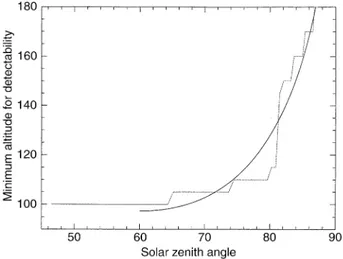
In the E region, EISCAT can detect electron densities above typically a few 1010m~3. We therefore checked at what altitude the TRANSCAR-computed electron density reaches the threshold of 5·1010m~3. This is shown in Fig. 2. Below 65°, the electron density only reaches such low values in the very low E region, where the conductan-ces are no longer important. At 66°, this threshold is above 100 km, and starts to affect the Hall conductance inferred from the EISCAT electron density measurement. It keeps going up to reach about 120 km at 75°. Then, the Pedersen conductivity also starts to be affected. The code covers the E region with 19 altitudes. The effect of the discretization is obvious in Fig. 2. We smoothed it with a simple polynomial which will be discussed in Sect. 4.
Fig. 2. Thebroken lineshows the altitude above which the electron density is larger than the threshold of detection for EISCAT in the E region. Thesmoothed linefollows the equationz"361.8568 coss! 511.5282 cos0.5s#278.1 for solar anglesslarger than 60°
The conclusion of this section is that EISCAT has some difficulties in determining the conductances only due to solar photoionization typically above 65°solar angle from the power-profile measurement or for typical integration times of few minutes. What Senior (1991) has seen are conductivities due to particle precipitation, as confirmed by the statistical model of Hardy et al. (1985, 1987). At angles where the ion production due to photoionization is larger than the detectability threshold at all altitudes in the E region, our model fits the CS prediction very nicely. This may be confirmed by a comparison between CS (and the other models) and a DMSP/Sondrestrom coordinated experiment (Watermannet al., 1993). In this paper, height-integrated electrical conductivities are deduced using radar and spacecraft measurements in combination with atmospheric and ionospheric models to distinguish be-tween the contribution of the two main sources of ioniza-tion of the thermosphere during solar minimum. What is found is that for angles above 60°, the solar radiation components of the Pedersen and Hall conductances are systematically overestimated by the models in about the same proportion as that found in the present study. We therefore think that TRANSCAR proves to be a useful tool for modeling diurnal conductivities.
3 Influence of various parameters
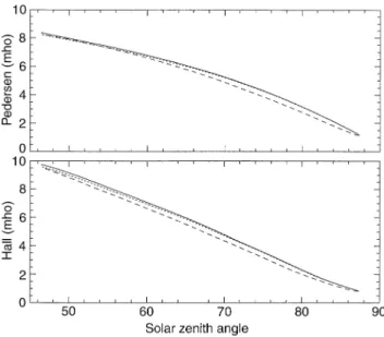
In this next section, we replace all the specific parameters used by Senior (1991) for her statistical study by the usual parameters: the ion mass and the magnetic field intensity depend on the altitude, the neutral atmosphere is MSIS 90 (Hedin, 1991), the ion/collision frequencies depend on the ion temperature (see for example the review by Brekke and Moen, 1993), the integration upper limit is 600 instead of 200 km, the electron and ion temperatures are never set to the neutral one but computed by TRANSCAR. All these changes lead, of course, to a big change in the results, as shown in Fig. 3. In this figure, the conductivities are com-puted in the evening sector, the solar angle increasing from 45°to 86°, so that the comparison makes sense. It results in an increase in the Pedersen conductivity of about 0.6 to 0.7 MHO at low angle and 0.2 MHO at 87°, and a decrease in the Hall conductivity reaching 1.3 MHO at low angle. This is mostly an effect of the neutral atmosphere model. The differences between vin2mil and MSIS will not be discussed here, this being beyond the scope of this paper.
Fig. 3. Hall and Pedersen integrated conductivities. Thedashed line
represents the results of TRANSCAR computation with Senior’s parameters. Thedot-dashed lineis the same computation with usual parameters (see text). Thefull lineshows CS model
Brekke and Hall (1988) have already studied the influ-ence of the set of collision frequencies. That will therefore not be repeated here since our study agrees fairly well with their conclusions. They note that for the collision fre-quency model given by version 1 used in CS, the Pedersen profile has its maximum at greater heights than for the model given by version 2 (with ¹
e-dependent collision frequencies), and that the Hall conductivity profile is en-hanced at greater heights for model 1 than for model 2. Their study and comparison with experiment use model 2. Table 1 shows the influence of the variation of several parameters in the computation of the conductances. The magnetic field directly influences the conductivities, as well as indirectly through the gyrofrequencies. Its vari-ation then has an important effect on the conductivities: increasing it by 5% leads to a decrease of about 10% in the Hall and 8.7% in the Pedersen conductance. An ion composition made up of 100% O`2 or NO`ions has little influence on the Hall conductance, but strongly increases the Pedersen conductance. In the test run, the composi-tion is as follows: we compute the O`composition (which is of course unimportant at such low altitudes) from the time dependent model from Chantal Lathuille`re (Blelly et al., 1996), and then make the assumption that the mo-lecular ions are made up of 50% O`2 and 50% NO`. Changing this ratio has little influence on the global ion mass but changes the ion/neutral collision frequencies. The multiplication of the collision frequencies by a factor of 2 increases the Hall conductance by about 38% and the Pedersen conductance by about 30%. Since the O`ion is not abundant at altitudes where the conductivities are large, the Burnside factor has almost no influence.
In Fig. 5 we plotted the reference computation (based on ‘‘usual’’ parameters and for day 183) versus the compu-tation for day 80, in order to check the influence of the period of the year on the conductivities at a given solar
Fig. 4. The panel on thetopshows the height profile of the Hall (dashed line) and Pedersen (dotted line) conductances, obtained by averaging a 12-h run of our model. Thebottom panel shows the percentage of explanation of the conductances versus altitude
Table 1. Numerical influence of several parameters on a given ‘‘representative’’ run
Hall conductance Pedersen conductance
Test run 6.448 5.876
1.05B 5.801 5.36
100% O 6.664 7.196
100% NO` 6.606 7.052
2l
*/ 8.894 7.638
Burnside"1 6.440 5.763
zenith angle. On day 80, the solar angle only rises to 70°; the effect on the Hall conductance is negligible, but the Pedersen conductance increases by about 0.5 MHO due to the change in the neutral atmosphere. In the same plot we show the effect of theApindex; for the test run it is set to 14. We show the conductances for Ap"3 and 20, which are typical margin values for f
Fig. 5. The full line is the TRANSCAR computation with usual parameters. The thin-dashed line is the same computation with
Ap"20. The dotted linerepresents the computation for Ap"3. Finally, thelarge-dashed lineis the computation for day 80
Fig. 6. Morning (dashed lines)/evening (full and dotted lines) conduc-tances; see text for further details
Figure 6 shows the conductances computed with ‘‘usual’’ parameters for a 36-h run starting at 12 UT on 21 June and ending at 24 UT on 22 June. The neutral atmo-sphere given by MSIS is not the same in the morning and evening, so that the conductivities may be different at a given solar zenith angle in the evening and in the morning sectors. We therefore kept apart the conductivi-ties from the two afternoons and from the morning of 22 June. This figure reads starting at 12 UT on 21 June on the top left corner of each panel; it follows the full line to go to sunset on the lower right part of each panel. Then the sun rises again on 22 June and the conductivities follow the dashed lines towards the left. An angle of 70°is obtained at 18.3 LT on the full line and at 5.7 LT on the dashed line.
Finally, one passes midday at noon on 22 June and goes to midnight: the conductances are then represented by the dotted lines.
At equal solar zenith angle, the evening (from noon to midnight, full and dotted lines) Pedersen conductance is up to 0.4 MHO larger than in the morning (from midnight to noon, dashed line), which represents a relative variation of about 10% at a solar zenith angle of 70° on the Pedersen conductance. The effect on the Hall conductance is not as large as on Pedersen (about 5% maximum), but lasts for a larger range of solar angles (from 50°to 80°). This morning/evening effect has been already found ex-perimentally by Senior (1980), using data from the French incoherent-scatter radar in Saint Santin. The modeled and experimental morning/evening asymmetries agree very well. From one day to the next, there is a small difference at noon of about 0.1 MHO on the Pedersen and 0.2 MHO on the Hall conductance. This difference vanishes as one approaches large angles. This is mainly an effect of the neutral atmosphere: on day 183, one reaches large angles. This is mainly an effect of the neutral atmosphere: on day 183, one reaches the solar zenith angle of 46.58°, while the minimum angle is 46.66°the next day. Even such a small difference produces relative differences of about 0.1% on the neutral temperatures and densities given by MSIS90. This difference is maximum for O
2and for the temper-ature at 110 km, affecting the Hall more than the Pedersen conductivity. The effect is enhanced by the fact that the neutral atmosphere enters the computation of the conductivities through the collision frequencies in the denominator only for the Hall conductance, but on both denominator and numerator for the Pedersen conduc-tance (Eqs. 1 and 2).
4 EISCAT and ESR conductances
We ran our code for different solar activity levels at EISCAT and ESR latitudes. We show here the result of this modeling of the evening conductances, in order to propose a simple model depending only on the solar zenith angle. In order to use to compare with instan-taneous measurements, one should use the study of the preceding section to proceed to corrections.
We varied the f
10.7index; as shown earlier, the effect of varying theApindex is small, but exists especially for the Pedersen conductances. We therefore varied Ap at the same time as the f
10.7index. To do this we averaged the Ap indices of the last solar cycle at each monthly f
10.7 index. Table 2 shows this variation ofApversus f
10.7and the numbers used in our modeling.
Table 2.Variation of theApindex versus f
10.7
Sf
10.7T Months ofoccurrences SApT SApusedT
70 21 13.3 13.5
80 21 14.85 14
90 12 14.75 14.5
100 9 15.3 15
110 5 13.2 15.5
120 7 17.85 16
130 7 18.6 16.5
140 5 13.6 17
150 1 12 17.5
160 2 10.5 18
170 3 20 18.5
180 6 16.2 19
190 5 19.6 19.5
200 9 20.1 20
210 5 22 20.5
220 2 19 21
230 6 20.5 21.5
Table 3.The coefficients for our fitted law of conductances
EISCAT EISCAT ESR ESR
Hall Pedersen Hall Pedersen
a
1 0.085 0.006 0.109 !0.004
a
2 8.697 2.048 4.713 !0.017
b
1 !0.022 0.061 !0.051 0.080
b
2 0.222 3.990 4.300 6.331
c
1 0.002 !0.003 0.009 !0.014
c
2 0.227 !0.560 !0.858 !1.205
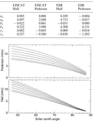
Fig. 7. We show the conductances versus solar zenith angle for seven different solar activities (from bottom to top: f
10.7"70, 80,
100, 120, 140, 160, 180) fitted with a second-order polynomial in cos0.5s
an offset. The variation of the coefficients versus f 10.7was considered to be linear (other dependencies proved not to be as precise), so that the generic formula gives:
RH,P"(a
1f10.7#a2) coss#(b1f10.7#b2) cos0.5s #(c
1f10.7#c2) (5)
Fig. 8. Same as Fig. 7 above ESR
The coefficients a, b, and c are given in Table 3 for EISCAT and ESR, while Figs. 7 and 8 show the conduc-tances for seven different activity levels at Tromso¨ and Svalbard latitudes (f
10.7"70, 80, 100, 120, 140, 160, and 180). The proposed law follows TRANSCAR modeling to less than 5% at any solar angle. The diurnal conductances due solely to photoionization that we predict over ESR are slightly smaller than the conductances over EISCAT for a given solar zenith angle.
Finally, since the conductivity is proportional to the electron density, it is natural to model the altitude below which the electron density is smaller than 5.1010m~3, i.e., is no longer detectable by EISCAT (using typical integra-tion times up to 5 mm) by the same kind of laws. This is shown in Fig. 2 as a smoothed line. For solar zenith angles larger than 60°, we found that z"361.8568 coss! 511.5282 cos0.5s#278.1 allows us to compute easily such an altitude.
5 Conclusion
We performed a modeling of the conductances above EISCAT and, in a predictive manner, above ESR, using a coupled fluid/kinetic approach. In order to do so, we first compared successfully our results to the statistical experimental work of Senior (1991). We have shown that EISCAT cannot determine the conductances only due to the solar photoionization for high solar zenith angles with the usual integration times of 1—5 min. Then we studied the influence of various parameters, and finally, we could fit the Hall and Pedersen conductances with a simple second-order polynomial in cos0.5s. The coefficients of these polynomials depend on the solar activity level f
10.7. This work will be continued in the near future by comput-ing an hour/latitude/activity level conductance model.
research councils of Finland (SA), France (CNRS), the Federal Republic of Germany (MPG), Norway (NAVF), Sweden (NFR), and the United Kingdom (SERC). We thank Catherine Senior, who kindly gave us her data base and always accepted to discuss our results. We thank also Vincent Wickwar and Chantal Lathuille`re for their interest in this research. (French translation for French-speak-ing people: Nous remercions Catherine Senior pour nous avoir gentiment fourni sa base de donne´es et pour avoir toujours accepte´ de discuter nos re´sultats. Nous remercions aussi Vincent Wickwar et Chantal Lathuille`re pour l’inte´reˆt qu’ils ont porte´ a` notre travail.)
The Editor-in-Chief thanks R. Robinson and K. Freeman for their help in evaluating this paper.
References
Alcayde´, D.,An analytical static model of temperature and composi-tion from 20 to 2000 km altitude,Ann.Geophysicae,37,515—528, 1981.
Banks, P. M., and G. Kockarts,Aeronomy,Parts A and B, Academic Press, New York, 1973.
Barrett, J. L., and P. B. Hays,Spatial distribution of energy deposi-ted in nitrogen by electrons,J.Chem.Phys.,64,743, 1976.
Beaujardie`re, O. de-la, O. R. Johnson, and V. B. Wickwar, Ground-based measurements of Joule heating rates, inAuroral Physics, Eds. C. I. Meng, M. J. Rycroft, and L. A. Frank, Cambridge University Press, 1991.
Bjorna, N., B. Hultqvist, W. Kofman, J. Ro¨ttger, K. Schleel, T. Turunen, and D. M. Willis,¹he Eiscat Svalbard Radar, EIS-CAT council report, 1991.
Blelly, P-L., J. Lilensten, A. Robineau, J. Fontanari, and D. Alcayde´,
Callibration of a numerical ionospheric model with EISCAT observations, submitted toAnn.Geophysicae, 1996.
Brekke, A., and C. Hall, Auroral ionospheric quiet summertime conductances,Ann.Geophysicae,6,361—376, 1988.
Brekke, A., and J. Moen,Observations of high-latitude ionospheric conductances,J.Atmos.¹err.Phys.,55,1493—1512, 1993.
Brekke, A., and C. L. Rino,High-resolution altitude profiles of the auroral zone energy dissipation due to ionospheric currents,
J.Geophys.Res.,83,2517—2524, 1978.
Diloy, P. Y., A. Robineau, J. Lilensten, and J. Fontanari,A numerical model of ionosphere including the E region above EISCAT,Ann.
Geophysicae,14,191—200, 1996.
Green, A. E. S., C. S. Lindenmeyer, and M. Griggs,Molecular absorp-tion in planetary atmospheres,J.Geophys.Res.,69,493—504, 1964.
Hardy, D. A., M. S. Gussenhoven, and E. Holeman,A statistical model of auroral electron precipitation,J.Geophys.Res.,90,A5, 4229—4248, 1985.
Hardy, D. A., M. S. Gussenhoven, R. Raistrick, and W. J. McNeil,
Statistical and functional representations of the pattern of aur-oral energy flux and conductivity, J. Geophys. Res., 92,
12275—12294, 1987.
Hedin, A. E.,Extension of the MSIS thermosphere model into the middle and lower atmosphere,J.Geophys.Res.,96,1159, 1991.
Lummerzheim, D., and J. Lilensten,Electron transport and energy degradation in the ionosphere: evaluation of the numerical solu-tion, comparison with laboratory experiments and auroral ob-servations,Ann.Geophysicae,12,1039—1051, 1994.
Rishbeth, H., and A. P. van Eyken,EISCAT: early history and the first ten years of operation,J.Atmos.¹err.Phys.,55,525—542, 1993.
Robineau, A., P. L. Blelly, D. Alcayde´, and J. Fontanari,Plasma transports in the ionosphere, EISCAT-VHF observations and numerical models,J.Geomagn.Geoelectr.,47,847—860, 1995.
Robineau, A., P. L. Blelly, and J. Fontanari,Time-dependent models of the auroral ionosphere above EISCAT,J.Atmos.¹err.Phys.,
58,257—271, 1996.
Robinson, R. M., P. R. Vondrak, K. Miller, T. Dabbs, and D. A. Hardy,On calculating ionospheric conductivities from the flux and energy of precipitating electrons,J.Geophys.Res.,92,A5, 2565, 1987.
Schlegel, K.,Auroral zone E-region conductivities during solar min-imum derived from EISCAT data,Ann.Geophysicae,6,129—138, 1988.
Senior, C., Les conductivite´s ionosphe´riques et leur roˆle dans la convection magne´tosphe´rique: Une e´tude expe´rimentale et the´orique,¹he%se de troisie%me cycle, Universite´ P. et M. Curie, Paris 6, 1980.
Senior, C.,Solar and particle contributions to auroral height-inte-grated conductivities from EISCAT data: a statistical study,Ann.
Geophysicae,9,449—460, 1991.
Smith, F. L., and C. Smith, Numerical evaluation of Chapman’s grazing incidence itegral ch(x,s), J. Geophys. Res., 77,
3592—3597, 1972.
Spiro, R. W., P. H. Reiff, and L. J. Maher Jr.,Precipitating electron energy flux and auroral zone conductances: an empirical model,
J.Geophys.Res.,87,8215, 1982.
Tobiska, W. K.,Recent solar extreme ultraviolet irradiance observa-tions and modeling: a review,J.Geophys.Res.,98,18 879—18 893, 1993.
Torr, M. R., and D. J. Torr,Ionization frequencies for solar cycle 21: Revised,J.Geophys.Res.,90,6675—6678, 1985.
Waterman, J., O. de la Beaujardie`re, and F. J. Rich,Comparsion of ionospheric electrical conductances inferred from coincident radar and spacecraft measurements and photoionization models,
J.Atmos.¹err.Phys.,55,1513—1520, 1993.