Feedback Calibrate Motor-Sensory Interval Timing
Luigi Acerbi1,2*, Daniel M. Wolpert3, Sethu Vijayakumar1
1Institute of Perception, Action and Behaviour, School of Informatics, University of Edinburgh, Edinburgh, United Kingdom, 2Doctoral Training Centre in Neuroinformatics and Computational Neuroscience, School of Informatics, University of Edinburgh, Edinburgh, United Kingdom,3Computational and Biological Learning Lab, Department of Engineering, University of Cambridge, Cambridge, United Kingdom
Abstract
Humans have been shown to adapt to the temporal statistics of timing tasks so as to optimize the accuracy of their responses, in agreement with the predictions of Bayesian integration. This suggests that they build an internal representation of both the experimentally imposed distribution of time intervals (the prior) and of the error (the loss function). The responses of a Bayesian ideal observer depend crucially on these internal representations, which have only been previously studied for simple distributions. To study the nature of these representations we asked subjects to reproduce time intervals drawn from underlying temporal distributions of varying complexity, from uniform to highly skewed or bimodal while also varying the error mapping that determined the performance feedback. Interval reproduction times were affected by both the distribution and feedback, in good agreement with a performance-optimizing Bayesian observer and actor model. Bayesian model comparison highlighted that subjects were integrating the provided feedback and represented the experimental distribution with a smoothed approximation. A nonparametric reconstruction of the subjective priors from the data shows that they are generally in agreement with the true distributions up to third-order moments, but with systematically heavier tails. In particular, higher-order statistical features (kurtosis, multimodality) seem much harder to acquire. Our findings suggest that humans have only minor constraints on learning lower-order statistical properties of unimodal (including peaked and skewed) distributions of time intervals under the guidance of corrective feedback, and that their behavior is well explained by Bayesian decision theory.
Citation:Acerbi L, Wolpert DM, Vijayakumar S (2012) Internal Representations of Temporal Statistics and Feedback Calibrate Motor-Sensory Interval Timing. PLoS Comput Biol 8(11): e1002771. doi:10.1371/journal.pcbi.1002771
Editor:Laurence T. Maloney, New York University, United States of America
ReceivedMay 25, 2012;AcceptedSeptember 24, 2012;PublishedNovember 29, 2012
Copyright:ß2012 Acerbi et al. This is an open-access article distributed under the terms of the Creative Commons Attribution License, which permits unrestricted use, distribution, and reproduction in any medium, provided the original author and source are credited.
Funding:This study was supported by an Engineering and Physical Sciences Research Council/Medical Research Council scholarship granted to LA from the Neuroinformatics and Computational Neuroscience Doctoral Training Centre at the University of Edinburgh. DMW is supported by the Wellcome Trust and the Human Frontiers Science Program. SV is supported through grants from Microsoft Research, Royal Academy of Engineering and EU FP7 programs. The funders had no role in study design, data collection and analysis, decision to publish, or preparation of the manuscript.
Competing Interests:The authors have declared that no competing interests exist.
* E-mail: [email protected]
Introduction
The ability to estimate motor-sensory time intervals in the subsecond range and react accordingly is fundamental in many behaviorally relevant circumstances [1], such as dodging a blow or assessing causality (‘was it me producing that noise?’). Since sensing of time intervals is inherently noisy [2], it is typically advantageous to enhance time estimates with previous knowledge of the temporal context. It has been shown in various timing experiments that humans can take into account some relevant temporal statistics of a task according to Bayesian decision theory, such as in sensorimotor coincidence timing [3], tactile simultaneity judgements [4], planning movement duration [5] and time interval estimation [6–8].
Most of these studies [3,4,6,8] exposed the participants to time intervals whose duration followed some simple distribution (e.g. a Gaussian or a uniform distribution), and then assumed that the subjects’ internal representation of it corresponded to the experimental distribution. As a more realistic working hypothesis, we can expect the observers to have acquired, after training, an internal representation of the statistics of the temporal intervals which is an approximation of the true, objective experimental
distribution. It can be argued that this approximation in most cases would be ‘similar enough’ to the true distribution, so that in practice the distinction between subjective and objective distribu-tion is an unnecessary complicadistribu-tion. This is not exact though, first of all because it is unknown whether the similarity assumption would hold for complex temporal distributions, and secondly because the specific form of the approximation can lead to observable differences in behavior even for simple cases (see Figure 1).
Bayesian decision theory (BDT) provides a neat and successful framework for representing the internal beliefs of an ideal observer in terms of a (subjective) prior distribution, and it gives a normative account on how the ideal observer should take action [14]. A large number of behavioral studies are consistent with a Bayesian interpretation [15–17] and some results suggest that human subjects build internal representations of priors and likelihoods [15,18,19] or likelihood and loss functions [20]. We therefore adopted BDT as a framework to infer the subjects’ acquired beliefs about the experimental distributions. However, the behavior of a Bayesian ideal observer depends crucially not only on the prior, but also on the likelihoods and the loss function, with an underlying degeneracy, i.e. distinct combinations of distributions can lead to the same empirical behavior [21]. It follows that a proper analysis of the internal representations cannot be separated from an appropriate modelling of the likelihoods and the loss function as well.
With this in mind, we analyzed the timing responses of human observers for progressively more complex temporal distributions of durations in a motor-sensory time interval reproduction task. We provided performance feedback (also known as ‘knowledge of results’, or KR) on a trial-by-trial basis, which constrained the loss function, speeded up learning and allowed the subjects to adjust their behavior, therefore providing an upper bound on human performance [22,23]. We carried out a full Bayesian model comparison analysis among a discrete set of candidate likelihoods, priors and loss functions in order to find the observer model most supported by the data, characterizing the behavior of each individual subject across multiple conditions. Having inferred the form of the likelihoods and loss functions for each subject, we could then perform a nonparametric reconstruction [24] of what the subjects’ prior distributions would look like under the assumptions of our framework and we compared them with the experimental distributions. The inferred priors suggest that people learn smoothed approximations of the experimental distributions which take into account not only mean and variance but also higher-order statistics, although some complex features (kurtosis,
bimodality) seem to deviate systematically from those of the experimental distribution.
Results
Subjects took part in a time interval reproduction task with performance feedback (trial structure depicted in Figure 2 top; see Methods for full details). On each trial subjects clicked a mouse button and, after a time interval (xms) that could vary from trial-to-trial, saw a yellow dot flash on the screen. They were then required to hold down the mouse button to reproduce the perceived interval between the original click and the flash. The duration of this mouse press constituted their response (rms) for that trial. Subjects received visual feedback on their performance, with an error bar that was displayed either to the left or right of a central zero-error line, depending on whether their response was shorter or longer than the true interval duration. In different experimental blocks we varied both the statistical distribution of the intervals,p(x), and the nature of the performance feedback, i.e. mapping between the interval/response pair and the error display, f(x,r), relative to the zero-error line. For each experi-mental block, subjects first performed training sessions until their performance was stable (around 500 to 1500 trials), followed by two test sessions (about 500 trials per session). Testing with a block was completed before starting a new one.
Different groups of subjects took part in five experiments, whose setup details are summarized in Table 1 (see also Methods). In brief, Experiment 1 represented a basic test for the experimental paradigm and modelling framework with simple (Uniform) distributions over different ranges. Experiment 2 compared subjects’ responses in a simple condition (Uniform) vs a complex one (Peaked, one interval was over-represented), over the same range of intervals. Experiment 3 verified the effect of feedback on subjects’ responses by imposing a different error mappingf(x,r). Experiment 4 tested subjects in a more extreme version of the Peaked distribution. Experiment 5 verified the limits of subjects’ capability of learning with bimodal distributions of intervals.
We first present the results of the first two experiments in a qualitative manner, and then describe a quantitative model. Results of the other three experiments that test specific aspects of the model or more complex distributions are presented thereafter.
Experiment 1: Uniform distributions over different ranges
In the first experiment the distribution of time intervals consisted of a set of six equally spaced discrete times with equal probability according to either a Short Uniform (450–825 ms) or Long Uniform (750–1125 ms) distribution. The order of these blocks was randomized across subjects. The feedback followed a Skewed error mapping fSk!
r{x
r . The ‘artificial’ response-dependent asymmetry in the Skewed mapping was chosen to test whether participants would integrate the provided feedback error into their decision process, as opposed to other possibly more natural forms of error, such as the Standard errorfSt!r{x or the Fractional error fFr!
r{x
x (see later, Bayesian model comparison).
We examined the mean bias in the response (mean reproduc-tion interval minus actual interval,rr{x, also termed ‘constant error’ in the psychophysical literature), as a function of the actual interval (Figure 3 top). Subjects’ responses showed a regression to the mean consistent with a Bayesian process that integrates the prior with sensory evidence [4,6,8,15]. That is, little bias was seen for intervals that matched the mean of the prior (637.5 ms for Author Summary
Human performance in a timing task depends on the context of recently experienced time intervals. In fact, people may use prior experience to improve their timing performance. Given the relevance of time for both sensing and acting in the world, how humans learn and represent temporal information is a fundamental question in neuroscience. Here, we ask subjects to reproduce the duration of time intervals drawn from different distribu-tions (different temporal contexts). We build a set of models of how people might behave in such a timing task, depending on how they are representing the temporal context. Comparison between models and data allows us to establish that in general subjects are integrating task-relevant temporal information with the provided error feedback to enhance their timing performance. Analysis of the subjects’ responses allows us to reconstruct their internal representation of the temporal context, and we compare it with the true distribution. We find that with the help of corrective feedback humans can learn good approximations of unimodal distributions of time intervals used in the experiment, even for skewed distributions of durations; on the other hand, under similar conditions, we find that multimodal distributions of timing intervals are much harder to acquire.
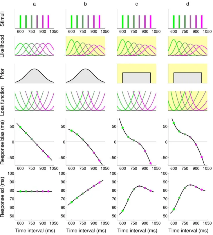
Figure 1. Comparison of response profiles for different ideal observers in the timing task.The responses of four different ideal observers (columnsa–d) to a discrete set of possible stimuli durations are shown (top row); for visualization purpose, each stimulus duration in this plot is associated with a specific color. The behavior crucially depends on the combination of the modelled observer’s temporal sensorimotor noise (likelihood), prior expectations and loss function (rows2–4); see Figure 2 bottom for a description of the observer model. For instance, the observer’s sensorimotor variability could be constant across all time intervals (column a) or grow linearly in the interval, according to the ‘scalar’ property of interval timing (column b–d). An observer could be approximating the true, discrete distribution of intervals as a Gaussian (columns a–b) or with a uniform distribution (columns c–d). Moreover, the observer could be minimizing a typical quadratic loss function (columns a–c) or a skewed cost imposed through an external source of feedback (column d). Yellow shading highlights the changes of each model (column) from model (a). All changes to the observer’s model components considerably affect the statistics of the predicted responses, summarized by response bias, i.e. average difference between the response and true stimulus duration, and standard deviation (bottom two rows). For instance, all models predict a central tendency in the response (that is, a bias that shifts responses approximately towards the center of the interval range), but bias profiles show characteristic differences between models.
Short Uniform, red points, and 937.5 ms for Long Uniform, green points). However, at other intervals a bias was seen towards the mean interval of that experimental block, with subjects reporting intervals longer than the mean as shorter than they really were and conversely intervals shorter than the mean as being longer than they really were. Moreover, this bias increased almost linearly with the difference between the mean interval and the actual interval. Qualitatively, this bias profile is consistent with most reasonable hypotheses for the prior, likelihoods and
loss functions of an ideal Bayesian observer (even though details may differ).
The standard deviation of the response (Figure 3 bottom) showed a roughly linear increase with interval duration, in agreement with the ‘scalar property’ of interval timing [25], according to which the variability in a timing task grows in proportion to the interval duration.
These results qualitatively suggest that the temporal context influences subjects’ performance in the motor-sensory timing task in a way which may be compatible with a Bayesian interpretation,
Figure 2. Time interval reproduction task and generative model.Top:Outline of a trial. Participants clicked on a mouse button and a yellow dot was flashedxms later at the center of the screen, withxdrawn from a block-dependent distribution (estimation phase). The subject then pressed the mouse button for a matching duration ofrms (reproduction phase). Performance feedback was then displayed according to an error mapf(x,r).Bottom:Generative model for the time interval reproduction task. The intervalxis drawn from the probability distributionp(x)(the
objective distribution). The stimulus induces in the observer the noisy sensory measurementywith conditional probability densityps(yDx;ws)(the
sensory likelihood), withws a sensory variability parameter. The actionusubsequently taken by the ideal observer is assumed to be the ‘optimal’ actionuthat minimizes the subjectively expected loss (Eq. 1);uis therefore a deterministic function ofy,u~u(y). The subjectively expected loss depends on terms such as the priorq(x)and the loss function (squared subjective error map~ff(x,r)), which do not necessarily match their objective counterparts. The chosen action is then corrupted by motor noise, producing the observed response r with conditional probability density pm(rDu; wm)(themotor likelihood), wherewmis a motor variability parameter.
doi:10.1371/journal.pcbi.1002771.g002
and in agreement with previous work which considered purely sensory intervals and uniform distributions [6,8,26].
Experiment 2: Uniform and Peaked distributions on the same range
As in the first experiment six different equally-spaced intervals were used, with two different distributions. However, in this experiment both blocks had the same range of intervals (Medium: 600–975 ms). In one block (Medium Peaked) one of the intervals (termed the ‘peak’) occurred more frequently than the other 5 intervals, that were equiprobable. That is, the 675 ms interval occurred withp~7=12with the other 5 intervals occurring each with p~1=12. In the other block (Medium Uniform) the 6 intervals were equiprobable. The feedback gain for both blocks was again the Skewed error mapfSk!
r{x r .
Examination of the responses showed a central tendency as encountered in the previous experiment (Figure 4 top). However, despite the identical range of intervals in both blocks, subjects were sensitive to the relative probability of the intervals [27]. In particular, the responses in the Peaked block (light blue points) appeared to be generally shifted towards shorter durations and this shift was interval dependent (see Figure 5). This behavior is qualitatively consistent with a simple Bayesian inference process, according to which the responses are ‘attracted’ towards the regions of the prior distribution with greatest probability mass. Intuitively, the average (‘global’) shift of responses can be thought of as arising from the shift in the distribution mean, from the Uniform distribution (mean 787.5 ms) to the Peaked distribution (mean 731.3 ms); whereas interval-dependent (‘local’) effects are a superimposed modulation by the probability mass assignments of the distribution. This is only a simplified picture, as the biases depend on a nonlinear inference process, which is also influenced by other details of the Bayesian model (such as the loss function), but the qualitative outcome is likely to be similar in many relevant cases. The standard deviation of the responses showed a significant decrease in variability around the peak for the Peaked condition (Figure 4 bottom; two-sample F-testpv0:001). This effect could be simply due to practice as subjects received feedback more often at peak intervals, however the local modulation of bias previously described (Figure 5) suggests a Bayesian interpretation. In fact,
because of the local ‘attraction’ effect, interval durations close to the peak would elicit responses that map even closer to it, therefore compressing the perceptual variability, an example of bias-variance trade-off [6].
The results of the second experiment show that people take into account the different nature of the two experimental distributions, in agreement with previous work that found differential effects in temporal reproduction for skewed vs uniform distributions of temporal intervals on a wider, suprasecond range [27]. The performance of the subjects in the two blocks is consistent with a Bayesian ‘attraction’ in the response towards the intervals with higher prior probability mass. Moreover, although the average negative shift in the response observed in the Peaked condition versus the Uniform one might be compatible with a temporal recalibration effect that shortens the perceived duration between action and effect [11,28,29], the interval-dependent bias modula-tion (Figure 5) and the reducmodula-tion in variability around the peak (Figure 4 bottom) suggest there may instead be in this case a Bayesian explanation.
In order to address more specific, quantitative questions about our results we set up a formal framework based on a Bayesian observer and actor model.
Bayesian observer model
We modelled the subjects’ performance with a family of Bayesian ideal observer (and actor) models which incorporated both the perception (time interval estimation) and action (reproduction) components of the task; see Figure 2 (bottom) for a depiction of the generative model of the data. We assume that on a given trial a time interval x is drawn from a probability distributionp(x) (the experimental distribution) and the observer makes an internal measurement y that is corrupted by sensory noise according to thesensory likelihoodps(yDx;ws), where wsis a parameter that determines the sensory (estimation) variability. Subjects then reproduce the interval with a motor command of durationu. This command is corrupted by motor noise, producing the response durationr– the observed reproduction time interval – with conditional probability density pm(rDu; wm) (the motor
likelihood), withwm a motor (reproduction) variability parameter. Subjects receive an error specified by a mappingf(x,r)and we assume they try to minimize a (quadratic) loss based on this error.
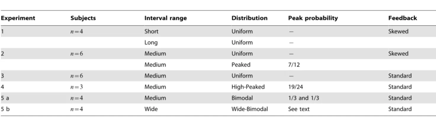
Table 1.Summary of experimental layout for all experiments.
Experiment Subjects Interval range Distribution Peak probability Feedback
1 n~4 Short Uniform { Skewed
Long Uniform {
2 n~6 Medium Uniform { Skewed
Medium Peaked 7/12
3 n~6 Medium Uniform { Standard
4 n~3 Medium High-Peaked 19/24 Standard
5 a n~4 Medium Bimodal 1/3 and 1/3 Standard
5 b n~4 Wide Wide-Bimodal See text Standard
Each line represents an experimental block, which are grouped by experiment; subjects in Experiment 1 and 2 took part in two blocks, whereas in Experiment 5 two distinct groups of subjects took part in the two blocks. For each block, the table reports number of subjects (n), interval ranges, type of distribution, probability of the ‘peak’ (i.e. most likely) intervals and shape of performance feedback. Tested ranges were Short (450–825 ms), Medium (600–975 ms), Long (750–1125 ms) and Wide (450–1125 ms), each covered by 6 intervals (10 for the Wide block) separated by 75 ms steps. Distributions of intervals were Uniform (1/6 probability per interval), Peaked/High-peaked (the ‘peak’ interval at 675 ms appeared with higher probability than non-peak stimuli, which were equiprobable), Bimodal (intervals at 600 and 975 ms appeared with higher probability) and Wide-Bimodal (intervals at 450–600 ms and 975–1125 ms appeared with higher probability). The Skewed feedback takes
the form!r{x
In our model we assume that subjects develop an internal estimate of both the experimental distribution and error mapping (the feedback associated with a response rto stimulus x), which leads to the construction of a (subjective) prior,q(x), and subjective error mapping~ff(x,r); the latter is then squared to obtain the loss function. This allows the prior and subjective error mapping to deviate from their objective counterparts, respectively p(x) and f(x,r).
Following Bayesian decision theory, the ‘optimal’ actionu(y) is
calculated as the actionuthat minimizes the subjectively expected loss:
u(y)~arg min
u
ð
ps(yDx; ws)q(x)pm(rDu; wm)~ff2(x,r)dx dr ð1Þ
where the integral on the right hand side is proportional to the subjectively expected loss. Combining Eq. 1 with the generative model of Figure 2 (bottom) we computed the distribution of responses of an ideal observer for a target time intervalx, integrating over the hidden
internal measurement y which was not directly accessible in our experiment.
Therefore the reproduction timer of an ideal observer, given the target intervalx, is distributed according to:
p(rDx; ws,wm)~
ð
ps(yDx; ws)pm(rDu(y);wm)dy: ð2Þ
Eqs. 1 and 2 are the key equations that allow us to simulate our task, in particular by computing the mean response bias and standard deviation of the response for each interval (Section 1 in Text S1). Eq. 1 represents the internal model and deterministic decision process adopted by the subject whereas Eq. 2 represents probabilistically the objective generative process of the data. Notice that the experimental distributionp(x)and objective error mappingf(x,r)do not appear in any equation: the distribution of responses of ideal observers only depends on their internal representations of prior and loss function.
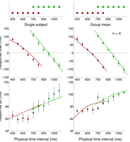
Figure 3. Experiment 1: Short Uniform and Long Uniform blocks.Very top:Experimental distributions for Short Uniform (red) and Long Uniform (green) blocks, repeated on top of both columns.Left column:Mean response bias (average difference between the response and true interval duration, top) and standard deviation of the response (bottom) for a representative subject in both blocks (red: Short Uniform; green: Long Uniform). Error bars denote s.e.m. Continuous lines represent the Bayesian model ‘fit’ obtained averaging the predictions of the most supported models (Bayesian model averaging).Right column:Mean response bias (top) and standard deviation of the response (bottom) across subjects in both blocks (mean+s.e.m. across subjects). Continuous lines represent the Bayesian model ‘fit’ obtained averaging the predictions of the most supported models across subjects.
doi:10.1371/journal.pcbi.1002771.g003
Eqs. 1 and 2 describe afamilyof Bayesian observer models, a single Bayesian ideal observer is fully specified by picking (i) a noise model for the sensory estimation process,ps(yDx; ws); (ii) a noise model for the motor reproduction process pm(rDu;wm); (iii) the form of the priorq(x); and (iv) the loss function~ff2(x,r)(Figure 6 and Methods). To limit model complexity, in the majority of our analyses we used the same likelihood functions (ps,pm and their parametersws,wm) for both the generative model (Eq. 2) and the internal model (Eq. 1). Analogously, for computational reasons in our basic model we assumed a quadratic exponent for the loss function (Eq. 1); in a subsequent analysis we relaxed this requirement (Section 2 in Text S1).
Bayesian model comparison
To study the nature of the internal model adopted by the participants, we performed a full Bayesian model comparison over the family of Bayesian ideal observer models. For each participant we assumed that the sensory and motor noise, the approximation
strategy for the priors, and the loss function were shared across different experimental blocks. The model comparison was performed over a discrete set of model components, that is, possible choices for the priors, loss functions and shape of likelihoods (Figure 6). In particular, priors and loss functions did not have continuous parameters, as a parametric model would likely be ambiguous or hard to interpret, with multimodal posterior distributions over the parameters (as multiple combina-tions of likelihoods, prior and cost function can make identical predictions). Instead, we considered a finite number of parameter-free models of loss function, prior and shape of likelihoods, leaving only two continuous parameters for characterizing the sensory and motor variability.
Both sensory and motor noise were modelled with Gaussian distributions whose means were centered on the interval and whose standard deviations could either be constant or ‘scalar’, that is, grow linearly with the interval (Figure 6 i and ii). We used two parameters, ws and wm, which represent the coefficient of variation of the subject’s sensory and motor noise. For the scalar
Figure 4. Experiment 2: Medium Uniform and Medium Peaked blocks.Very top:Experimental distributions for Medium Uniform (light brown) and Medium Peaked (light blue) blocks, repeated on top of both columns.Left column:Mean response bias (average difference between the response and true interval duration, top) and standard deviation of the response (bottom) for a representative subject in both blocks (light blue: Medium Uniform; light brown: Medium Peaked). Error bars denote s.e.m. Continuous lines represent the Bayesian model ‘fit’ obtained averaging the predictions of the most supported models (Bayesian model averaging).Right column:Mean response bias (top) and standard deviation of the response (bottom) across subjects in both blocks (mean+s.e.m. across subjects). Continuous lines represent the Bayesian model ‘fit’ obtained averaging the predictions of the most supported models across subjects.
case this simply specifies the coefficient of proportionality of the standard deviation with respect to the mean, whereas in the constant case it specifies the proportion of noise with respect to a fixed interval (787.5 ms).
We considered three different possible subjective error metrics corresponding to the Skewed error~ffSk(x,r)!
r{x
r (the error map we provided experimentally), the Standard error ~ffSt(x,r)!r{x, and a Fractional error ~ffFr(x,r)!
r{x
x (Figure 6 iv), which were then squared to obtain the loss function (see also Methods). Note that scaling these mappings does not change the optimal actions and hence the model selection process.
We compared different approximation schemes for the priors, such as the true discrete distribution (Figure 6 iii, a) or a single Gaussian whose mean and standard deviation matched those of the true prior (b). We also considered two smoothed versions of the experimental distribution with a weak (c) and strong (d) smoothing parameter, or some other block-dependent approximations, e.g. for the Uniform blocks we considered a uniform distribution over the stimulus range (e); see Methods for a full description. To constrain the model selection process, we assumed that subjects adopted a consistent approximation scheme across blocks.
For each participant we computed the support for each model based on the psychophysical data, that is the posterior probability of the model, Pr(model| data). Assuming an a priori indifference among the models, this corresponds (up to a normalization factor) to the model marginal likelihood Pr(data| model), which was obtained by numerical integration over the two-dimensional parameter space (wsandwm).
We then calculated the Bayesian model average for the response mean bias and standard deviation, shown by the continuous lines in Figure 3 and 4. Note that the Bayesian model ‘fits’ are obtained by computing the marginal likelihood of the models and integrating the model predictions over the posterior of the parameters (model averaging), with no parameter fitting. The mean biases fits show a good quantitative match with the group averages (R2§0:95 for all blocks); the standard deviations are typically more erratic and we found mainly a qualitative agreement, as observed in previous work [6].
For each participant of Experiments 1 and 2 we computed the most probable (i) sensory and (ii) motor likelihoods, (iii) priors and (iv) loss function (Table S1). The model comparison confirmed that the best noise models were represented by the ‘scalar’ variability, which had relevant support for both the sensory component (7 subjects out of 10) and the motor component (8 subjects out of 10). This result is consistent with previous work in both the sensory and motor domain [5,6,25,30]. The most supported subjective error map was the Skewed error (7 subjects out of 10), which matched the feedback we provided experimen-tally. The priors most supported by the data were typically smooth, peaked versions of the experimental distributions. In particular, according to the model comparison, almost all subjects (9 out of 10) approximated the discrete uniform distributions in the Uniform blocks with normal distributions (same mean and variance as the true distribution; Figure 6 iii top, b). However, in Experiment 2 most people (5 out of 6) seemed to approximate the experimental distribution in the Peaked block not with a standard Gaussian, but with a skewed variant of a normal distribution (Figure 6 iii bottom, d, f and g), suggesting that their
Figure 5. Experiment 2: Difference in response between Medium Peaked and Medium Uniform blocks.Difference in response between the Medium Peaked and the Medium Uniform conditions as a function of the actual interval, averaged across subjects (+1s.e.m.). The experimental distributions (light brown: Medium Uniform; light blue: Medium Peaked) are plotted for reference at bottom of the figure. The dashed black line represents the average response shift (difference in response between blocks, averaged across all subjects and stimuli), with the shaded area denoting+s.e.m. The average response shift is significantly different from zero ({32:2+7:9ms; two-sample t-testpv10{7), meaning that the two
conditions elicited consistently different performance. Additionally, the responses were subject to a ‘local’ (i.e. interval-dependent) modulation superimposed to the average shift, that is, intervals close to the peak of the distribution (675 ms) were attracted towards it, in addition to the average shift, while intervals far away from the peak were less affected. (*) The response shift at 600 ms and 825 ms is significantly different from the average response shift;pv0:01.
doi:10.1371/journal.pcbi.1002771.g005
responses were influenced by higher order moments of the true distribution and not just the mean and variance (see Discussion).
For Experiment 2 we also relaxed some constraints on the priors, allowing the model selection to pick a Medium Uniform prior for the Medium Peaked block and vice versa. Nevertheless, the model comparison showed that the most supported models were still the ones in which the priors matched the block distribution, supporting our previous findings that subjects’ responses were consistent with the temporal context and changed when switching from one block to another (as visible in Figure 4).
Nonparametric reconstruction of the priors
To study in detail the internal representations, we relaxed the constraint on the priors. Rather than choosing from a fixed set of candidate priors (Figure 6 iii), we allowed the prior to vary over a much wider class of smooth, continuous distributions. We assumed that the noise models and loss function emerging from the model comparison were a good description of the subjects’ decision making and sensorimotor processing in the task. We therefore fixed these components of the observer’s model and inferred nonparametrically, on an individual basis, the shape of the priors most compatible with the measured responses (Figure 7; see Methods for details).
Examination of the recovered priors shows that the subjective distributions were significantly different from zero only over the range corresponding to the experimental distribution, with only occasional tails stretching outside the interval range (e.g. Figure 7 bottom left). This suggests that in general people were able to localize the stimulus range in the blocks. The priors did not typically take a bell-like shape, but rather we observed a more or less pronounced peak at the mean of the true distribution, with the remaining probability mass spread over the rest of the range. Interestingly, the group averages for the Uniform priors over the Short, Medium and Long ranges (Figure 7 top right, both, and bottom right, light brown) exhibit very similar, roughly symmet-rical shapes, shifted over the appropriate stimulus range. Conversely, the Peaked prior (Figure 7 bottom right, light blue) had a distinct, skewed shape.
To compare the inferred priors with the true distribution, we calculated their distribution moments (Table 2). We found that the first three moments of the inferred priors (in the table reported as mean, standard deviation and skewness) were statistically indistin-guishable from those of the true distributions for all experimental conditions (Hotelling’s multivariate one-sampleT2test consider-ing the joint distribution of mean, standard deviation and skewness against the true values; pw0:45 for all blocks). This result confirmed the previously stated hypothesis that participants had
Figure 6. Bayesian observer and actor model components.Candidate (i) sensory and (ii) motor likelihoods, independently chosen for the sensory and motor noise components of the model. The likelihoods are Gaussians with either constant or ‘scalar’ (i.e. homogeneous linear) variability. The amount of variability for the sensory (resp. motor) component is scaled by parameterws(resp.wm).iii) Candidate priors for the Medium Uniform (top) and Medium Peaked (bottom) blocks. The candidate priors for the Short Uniform (resp. Long Uniform) blocks are identical to those of the Medium Uniform block, shifted by 150 ms in the negative (resp. positive) direction. See Methods for a description of the priors.iv) Candidate subjective error maps. The graphs show the error as a function of the response duration, for different discrete stimuli (drawn in different colors). From top to bottom: Skewed error~ff
Sk(r,x)! r{x
r ; Standard error ~
ffSt(r,x)!r{x; and Fractional errorff~Fr(r,x)! r{x
x . The scale is irrelevant, as the model is invariant to rescaling of the error map. The squared subjective error map defines the loss function (as per Eq. 1).
developed an internal representation which included higher order moments and not just the mean and variance of the experimental distribution. However, when including the fourth moment (kurtosis) in the analysis, we observed a statistically significant deviation of the recovered priors with respect to the true distributions (Hotelling’sT2test with the joint distribution of the first four moments; pv10{4 for all blocks); in particular, the inferred priors seem to have more pronounced peaks and/or heavier tails. First of all, note that the heightened kurtosis is not an artifact due to the averaging process across subjects or the sampling process within subjects, as we averaged the moments computed for each sampled distribution (see Methods) rather than computing the moments of the average distribution. In other words, all recovered priors are (on average) heavy tailed, it’s not just the mean prior that it is ‘accidentally’ heavy tailed as a mixture of light-tailed distributions. So this result could mean that the subjects’ internal representations are actually heavy-tailed, for instance to allow for unexpected stimuli. However, there could be a simpler explanation that the presence of outliers arise from occasional trivial mistakes of the participants. We, therefore, considered a straightforward extension of our model which added the possibility of occasional ‘lapses’ with a lapse ratel, where the response in a lapse trial is simply modelled as a uniform distribution over a wide range of intervals (Section 3 in Text S1). In terms of marginal likelihood, generally the models with lapse performed better than the original models, but with no qualitative difference in the preferred model components. Cru-cially, we did not observe a significant change in the kurtosis of the recovered priors, ruling out the possibility that the heightened kurtosis had been caused by trivial outliers.
Our analysis therefore showed that, according to the inferred priors, people generally acquired internal representations that were smooth, heavy-tailed approximations to the experimental
distributions of intervals, in agreement up to the first three moments.
Experiment 3: Effect of the shape of feedback on the loss function
In our ideal observer model we compared three candidate loss functions: Skewed, Standard and Fractional (Figure 6 iv). The results of the model comparison in the first two experiments with Skewed feedback showed that there was a good match between experimentally provided feedback and subjective error metric. However, we could not rule out the possibility, albeit unlikely, that participants were ignoring the experimental feedback and following an internal error signal that just happened to be similar in shape to the Skewed error. We therefore performed an additional experiment to verify that subjects behavior is driven by the feedback provided.
We again used a Medium Uniform block but now with Standard errorf(x,r)!r{x as feedback (see Figure S5 in Text S2). The model comparison for this group showed that the responses of 4 subjects out of 6 were best explained with a Standard loss function. Moreover, no subject appeared to be using the Skewed loss function (Table S1). These results confirm that most people correctly integrate knowledge of results with sensory information in order to minimize the average (squared) error, or an empirically similar metric. Furthermore, all inferred individual priors showed a remarkable agreement with a smoothed approximation of the experimental distribution of intervals (Figure 8 top), suggesting that the Standard error feedback may be easier to use for learning. As in the previous experiments, the average moments of the inferred priors (up to skewness) were statistically indistinguishable from those of the true distribution, with a significant difference in the kurtosis (Table 3 left; Hotelling’sT2test, first three moments:pw0:95; first four moments:pv10{7).
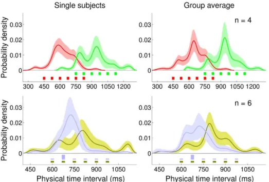
Figure 7. Nonparametrically inferred priors (Experiment 1 and 2).Top row:Short Uniform (red) and Long Uniform (green) blocks.Bottom row: Medium Uniform (light brown) and Medium Peaked (light blue) blocks.Left column: Nonparametrically inferred priors for representative participants.Right column:Average inferred priors. Shaded regions are+1s.d. For comparison, the discrete experimental distributions are plotted under the inferred priors.
doi:10.1371/journal.pcbi.1002771.g007
Experiment 4: High-Peaked distribution
In the Peaked block we did not observe any significant divergence from the Bayesian prediction. However, the ratio of presentations of ‘peak’ intervals (675 ms) to the others was low (1.4) and possibly not enough to induce other forms of temporal adaptation [29,31]. To examine whether we might see deviations from Bayesian integration for larger ratios we therefore tested another group of subjects on a more extreme variant of the Peaked distribution in which the peak stimulus had a probability ofp&0:8 and therefore a ratio of about 4.0. We provided feedback through
the Standard error mapping, as the previous experiment had showed that subjects can follow it at least as well as the Skewed mapping.
Due to the large peak interval presentation frequency we had fewer test data points in the model fitting. Therefore, we constrained the model comparison by only considering the Standard loss in order to prevent the emergence of spurious model components capturing random patterns in the data. We found that the recovered internal priors were in good qualitative agreement with the true distribution, with statistically
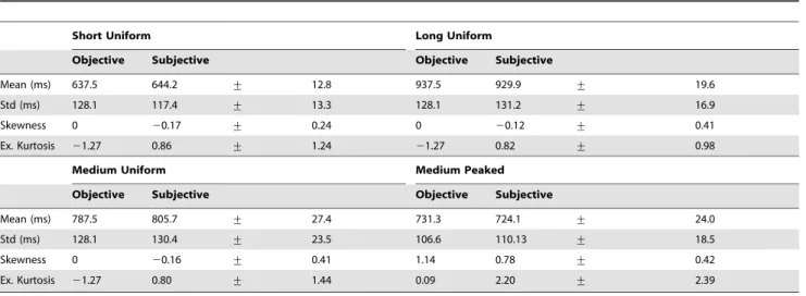
indistin-Table 2.Main statistics of the experimental distributions and nonparametrically inferred priors (Experiment 1 and 2; Skewed
feedback).
Short Uniform Long Uniform
Objective Subjective Objective Subjective
Mean (ms) 637.5 644.2 + 12.8 937.5 929.9 + 19.6
Std (ms) 128.1 117.4 + 13.3 128.1 131.2 + 16.9
Skewness 0 20.17 + 0.24 0 20.12 + 0.41
Ex. Kurtosis 21.27 0.86 + 1.24 21.27 0.82 + 0.98
Medium Uniform Medium Peaked
Objective Subjective Objective Subjective
Mean (ms) 787.5 805.7 + 27.4 731.3 724.1 + 24.0
Std (ms) 128.1 130.4 + 23.5 106.6 110.13 + 18.5
Skewness 0 20.16 + 0.41 1.14 0.78 + 0.42
Ex. Kurtosis 21.27 0.80 + 1.44 0.09 2.20 + 2.39
Comparison between the main statistics of the ‘objective’ experimental distributions and the ‘subjective’ priors nonparametrically inferred from the data. The subjective moments are computed by averaging the moments of sampled priors pooled from all subjects (+1s.d.); see Figure 7, right column and Methods for details. In statistics, the excess kurtosis is defined as kurtosis{3, such that the excess kurtosis of a normal distribution is zero. Heavy tailed distributions have a positive excess kurtosis. doi:10.1371/journal.pcbi.1002771.t002
Figure 8. Nonparametrically inferred priors (Experiment 3 and 4).Top row:Medium Uniform (light brown) block.Bottom row:Medium High-Peaked (dark blue) block.Left column:Nonparametrically inferred priors for representative participants.Right column:Average inferred priors. Shaded regions are+1s.d. For comparison, the discrete experimental distributions are plotted under the inferred priors.
guishable means (Figure 8 bottom, and Table 3; one sample two-tailed t-test pw0:90). When variance and higher moments were included in the analysis, though, the distributions were signifi-cantly different (Hotelling’sT2test, mean and variance:pv0:05; first three moments: pv0:01; first four moments: pv10{7) suggesting that the distribution may have been ‘too peaked’ to be learnt exactly; see Discussion. Nevertheless, the observed biases of the responses were well explained by the basic Bayesian models (group mean: R2~0:95), and the standard deviations were in qualitative agreement with the data (Figure S6 in Text S2).
Experiment 5: Bimodal distributions
Our previous experiments show that people are able to learn good approximation of flat or unimodal distributions of intervals relatively quickly (a few sessions), under the guidance of corrective feedback. Previous work in sensorimotor learning [15] and motion perception [32] has shown that people can learn bimodal distributions. Whether the same is attainable for temporal distributions is unclear; a recent study of time interval reproduc-tion [27] obtained less definite results with a bimodal ‘V-shaped’ distribution, although training might have been too short, as subjects were exposed only to 120 trials in total and without performance feedback.
To examine whether subjects could easily learn bimodality of a temporal distribution with the help of feedback we tested two new groups of subjects on bimodal distributions of intervals on a Medium range (600–975 ms, as before) and on a Wide range (450–1125 ms), providing in both cases Standard feedback. In the Medium Bimodal block the intervals at 600 and 975 ms had each probabilityp~4=12, whereas the other four middle intervals (675, 750, 825, 900 ms) had each probability p~1=12. In the Wide Bimodal block the six ‘extremal’ intervals (450, 525, 600 ms and 975, 1050, 1125 ms) had each probabilityp~4=28whereas the middle intervals had probability p~1=28. Note that in both cases extremal intervals were four times as frequent as middle intervals.
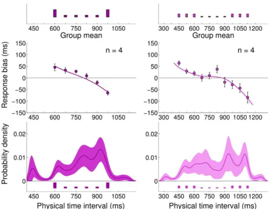
In the Medium Bimodal block, subjects’ responses exhibited a typical central tendency effect (Figure 9 top left) which suggests that people did not match the bimodality of the underlying distribution. To constrain the model comparison we inferred the subjects’ priors under the assumption of scalar sensory and motor noise models and Standard loss function, as found by our previous analyses. As before, we first used a discrete set of priors (see Methods) that we used to compute the model ‘fit’ to the data and then we performed a nonparametric inference. The nonparame-trically inferred priors for the Medium Bimodal distribution (Figure 9 top right) suggest that on average subjects developed an
internal representation that differed from those seen in previous experiments and, as before, we found a good agreement between moments of the experimental distribution and moments of the inferred priors up to skewness (Table 4 left). However, results of the Bayesian model comparison among a discrete class of flat, unimodal or bimodal priors do not support the hypothesis that subjects actually learnt the bimodality of the experimental distribution (data not shown). Part of the problem may have been that in the Medium Bimodal distribution the two modes were relatively close, and due to sensory and motor uncertainty subjects could not gather enough evidence that the experimental distribu-tion was not unimodal (but see Discussion). We repeated the experiment therefore on a wider range with a different group of subjects.
The pattern of subjects’ responses in the Wide Bimodal block shows a characteristic ‘S-shaped’ bias profile (Figure 9 top right) which is compatible with either a flat or a slightly bimodal prior. The nonparametrically inferred priors for the Wide Bimodal distribution (Figure 9 bottom right) again suggest that on average subjects acquired, albeit possibly with less accuracy (Table 4 right), some broad features of the experimental distribution; however individual datasets are quite noisy and again we did not find strong evidence for learning of bimodality.
Our results with bimodal distributions confirm our previous finding that people seem to be able to learn broad features of experimental distributions of intervals (mean, variance, skewness) with relative ease (a few sessions of training with feedback). However, more complex features (kurtosis, bimodality) seem to be much harder to learn (see Discussion).
Discussion
Our main finding is that humans, with the help of corrective feedback, are able to learn various statistical features of both simple (uniform, symmetric) and complex (peaked, asymmetric or bimodal) distributions of time intervals. In our experiments, the inferred internal representations were smooth, heavy tailed approximations of the experimental distributions, in agreement typically up to third-order moments. Moreover, our results suggest that people take into account the shape of the provided feedback and integrate it with knowledge of the statistics of the task in order to perform their actions.
The statistics of the responses of our subjects in the Uniform blocks were consistent with results from previous work; in particular, we found biases towards the mean of the range of intervals (central tendency) [6,8,26,33] and the variability of the responses grew roughly linearly in the sample interval duration (scalar property) [6,34]. The responses in the Peaked and
High-Table 3.Main statistics of the experimental distributions and nonparametrically inferred priors (Experiment 3 and 4; Standard
feedback).
Medium Uniform Medium High-Peaked
Objective Subjective Objective Subjective
Mean (ms) 787.5 782.6 + 18.7 703.1 702.0 + 17.9
Std (ms) 128.1 131.7 + 13.6 80.5 119.5 + 17.9
Skewness 0 0.03 + 0.30 2.25 0.67 + 0.37
Ex. Kurtosis 21.27 0.42 + 0.53 20.86 1.66 + 1.32
Comparison between the main statistics of the ‘objective’ experimental distributions and the ‘subjective’ priors nonparametrically inferred from the data. The subjective moments are computed by averaging the moments of sampled priors pooled from all subjects (+1s.d.); see Figure 8, right column and Methods for details. doi:10.1371/journal.pcbi.1002771.t003
Peaked blocks showed analogous biases, but they were directed towards the mean of the distribution rather than the mean of the range of intervals (the two means overlapped in the Uniform case) [27]. We also observed a significant reduction in variability at the peak. These results were sufficient to suggest that subjects considered the temporal statistics of the context in their decision making processes. We found a similar regression to the mean for a ‘narrow’ bimodal distribution (Medium Bimodal), in qualitative agreement with previous work that found a simple central tendency with a ‘V-shaped’ temporal distribution [27] (although with very limited training, no feedback and a suprasecond range). However, for a bimodal distribution on a wider range we observed ‘S-shaped’ biases which seem compatible with a nonlinear decision
making process [15]. However, more refined conclusions needed the support of a formal framework.
Bayesian model
Our modelling approach consisted of building a family of Bayesian observer and actor models, which provided us with a mathematical structure in which to ask specific questions about our subjects [35], going beyond mere statements about Bayesian optimality. In particular, we were interested in (1) whether people would be able to learn nontrivial temporal distributions of intervals and what approximations they might use, and (2) how their responses would be affected by performance feedback. Our observer model resembled the Bayesian Least Squares (BLS)
Figure 9. Experiment 5: Medium Bimodal and Wide Bimodal blocks, mean bias and nonparametrically inferred priors.Very top:
Experimental distributions for Medium Bimodal (dark purple, left) and Wide Bimodal (light purple, right) blocks.Top:Mean response bias across subjects (mean+s.e.m. across subjects) for the Medium Bimodal (left) and Wide Bimodal (right) blocks. Continuous lines represent the Bayesian model ‘fit’ obtained averaging the predictions of the most supported models across subjects.Bottom:Average inferred priors for the Medium Bimodal (left) and Wide Bimodal (right) blocks. Shaded regions are+1s.d. For comparison, the experimental distributions are plotted again under the inferred priors.
doi:10.1371/journal.pcbi.1002771.g009
Table 4.Main statistics of the experimental distributions and nonparametrically inferred priors for bimodal distributions
(Experiment 5; Standard feedback).
Medium Bimodal Wide Bimodal
Objective Subjective Objective Subjective
Mean (ms) 787.5 794.5 + 34.2 787.5 822.1 + 70.7
Std (ms) 160.6 155.7 + 37.2 251.6 219.2 + 29.3
Skewness 0 20.33 + 0.39 0 20.22 + 0.57
Ex. Kurtosis 21.72 20.08 + 0.90 21.64 20.40 + 0.51
Comparison between the main statistics of the ‘objective’ experimental distributions and the ‘subjective’ priors nonparametrically inferred from the data. The subjective moments are computed by averaging the moments of sampled priors pooled from all subjects (+1s.d.); see Figure 9, bottom and Methods for details.
observer described in [6], but it explicitly included an action component as part of the internal model. Moreover, to answer (1) we allowed the prior to differ from the experimental distribution, and to study (2) we considered additional shapes for the loss function in addition to the Standard squared loss!(r{x)2.
The Bayesian model comparison gave us specific answers for each of our subjects, and a first validation came from the success of the most supported Bayesian observer and actor models in capturing the statistics of the subjects’ responses in the task. However, goodness of fit per se is not necessarily an indicator that the components found by the model comparison reflected true findings about the subjects, rather than ‘overfitting’ arbitrary statistical relationships in the data. This is of particular relevance for Bayesian models, because of the underlying degeneracy among model components [21].
Our approach consisted in considering a large, ‘reasonable’ set of observer models that we could link to objective features of the experiment. This does not solve the degeneracy problem per se but it prevents the model comparison from finding arbitrary solutions. In particular, the set of experiments was designed in order to provide evidence that each element of the model mapped on to an experimentally verifiable counterpart; crucially, we found that a change in a component of the experimental setup (e.g. experi-mental distribution and feedback) correctly induced a switch in the corresponding inferred component of the model (prior and loss function). We also avoided overfitting by limiting our basic models to only two continuous noise parameters, which were then computed through model averaging and further validated by independent direct measures.
To further validate our methods, we directly measured the subject’s noise parameters (sensory and motor noise,w0sandw
0
m) in separate tasks and compared them with the model parametersws,
wminferred from the main experiments (see Section 4.1 in Text S1 for full description). The rationale is that, in an idealized situation, we would be able to measure some features of the subjects with an objective, independent procedure and the same features would be predictive of the individual performances in related tasks [16]. The measured parameters were highly predictive of the group behavior, and reasonably predictive at the individual level for the sensory parameter, confirming that the model parameters were overall correctly representing objective ‘noise properties’ of the subjects.
Overall, our modelling techniques were therefore validated by (a) goodness of fit, (b) consistency between inferred model components and experimental manipulations, and (c) consistency between the model parameters and independent measurements of the same quantities.
Comparison between inferred priors and experimental distributions
Given the validation of the results of the model comparison, we performed a nonparametric inference of the priors acquired by participants during the task. Other recent works have inferred the shape of subjective ‘natural’ perceptual priors nonparametrically, such as in visual orientation [24] and speed [36] perception, but studies that focussed on experimentally acquired priors mostly recovered them under parametric models (e.g. Gaussian priors with variable mean and variance) [35,37–39]. The nonparametric method allowed us to study the accuracy of the subjects in learning the experimental distributions, comparing summary statistics such as the moments of the distributions up to fourth order. Note that the significance and reliability of the recovered priors is based on the correctness of our assumptions regarding the observer and actor model; unconstrained priors might capture all sorts of
statistical details, one of the typical objections to Bayesian modelling [40]. However, by dividing the model selection stage (and its validation) from the prior reconstruction process we prevented the most pathological forms of overfitting.
The internal representations inferred from the data show a good agreement with the central moments of the true distributions typically up to third order (mean, variance and skewness). Subjects however showed some difficulties in learning variance and skewness when the provided distribution was extremely peaked, with a width less than the subjects’ perceptual variability. This discrepancy observed in the High-Peaked block may have arisen because (a) the experimental distribution’s standard deviation was equal or lower in magnitude compared to the perceptual variability of the subjects (experimental distribution standard deviation: 80.5 ms; subject’s average sensory standard deviation at the mean of the distribution:96:1+12:1ms; mean+sd across subjects) and (b) due to the shape of the distribution, subjects had much less practice with intervals away from the peak. Another explanation is that subjects’ representation of relative frequencies of different time intervals was systematically distorted, with overestimation of small relative frequencies and underestimation of large relative frequencies (see [41] for a critical review), but note that this would arguably produce a change in the mean of the distribution as well, which we did not observe.
Moreover, the recovered priors in all blocks had systematically heavier tails (higher kurtosis) than the true distributions. By exploring an extended model that included lapses we ruled out that this particular result was due to trivial outliers in our datasets. However, our results are compatible with other more sophisticated reasons for the heavy tails we recovered, in particular (a) the objective likelihoods might be non-Gaussian, with heavier tails [42], and (b) the loss functions might follow a less-than-quadratic power law [43], hypothesis for which we found some evidence, although inconclusive, by studying observer models with non-quadratic loss functions (Section 2 in Text S1). Experimentally, both (a) and (b) would imply that in our datasets there would be more outliers than we would expect from a Gaussian noise model with quadratic losses.
Our experiments with bimodal distributions show that, although people’s responses were affected by the experimental distribution of intervals in a way which is clearly different from our previous experiments with uniform or peaked distributions, the inferred priors in general fail to capture bimodality and are consistent instead with a broad uniform or multimodal prior (where the peaks however do not necessarily fall at the right places). Note that the average sensory standard deviation for subjects in Experiment 5 was87+18ms (Medium Bimodal; mean+sd across subjects) and106+28ms (Wide Bimodal), calculated at the center of the interval range. In other words, in both blocks, the centers of the peaks were well-separated in terms of perceptual discriminability (on average by at least four standard deviations). This suggests that most subjects did not simply fail to learn the bimodality of the distributions because they had problems distinguishing between the two peaks.
Temporal recalibration and feedback
prior expectations represented by the sample distribution of adaptation and test intervals, since its signature is a ‘repulsion’ from the adapter as opposed to the ‘attraction’ induced by a prior [4,47,48].
Our experimental setup for the peaked blocks mimicked the distributions of intervals of typical lag adaptation experiments [11,29], with the adapter interval set at 675 ms (the ‘peak’). However, we did not detect any noticeable disagreement with the predictions of our Bayesian observer model and, in particular, there was no significant ‘repulsion effect’ from the peak, neither global nor local. Our results suggest that people are not subject to the effects of lag adaptation, or can easily compensate for them, in the presence of corrective feedback.
Sensorimotor lag adaptation seems to belong to a more general class of phenomena of temporal recalibration which induce an adjustment of the produced (or estimated) timing of motor commands to meet the goals of the task at hand. In the case of experimentally induced actuator delays in a time-critical task, such as controlling a spaceship through a minefield in a videogame [49] or driving a car in a simulated environment [50], visual temporal information about delays provides an obvious, compelling reason to recalibrate the timing of actions. However, feedback regarding timing performance need not be provided only in temporal ways. Previous studies have shown that people take into account performance feedback (knowledge of results) when the feedback about the timing of their motor response is provided in various ways, such as verbal or visual report in milliseconds [23,51] or bars of variable length [52]. Interestingly, people tend to also follow ‘erroneous’ feedback [52–54]. However, this can be explained by the fact that people’s behavior in a timing task is goal-oriented (e.g. minimizing feedback error), and therefore these experiments suggest that people are able to follow external, rather than erroneous, feedback. In fact, when participants are told that feedback might sometimes be incorrect, which corresponds to setting different expectations regarding the goal of the task, they adjust their timing estimates taking feedback less into account [53]. Ambiguity regarding the goal of a timing task with non-obvious consequences – as opposed to actions that have obvious sensorimotor consequences, such as catching a ball – can be reduced by imposing an explicit gain/loss function [5,55], and it has been found that people can act according to an externally presented asymmetric cost (even though their timing behavior is not necessarily ‘optimal’ [55]).
Our work extends these previous findings by performing a model comparison with different types of symmetric and asymmetric loss functions and providing additional evidence that most people are able to correctly integrate an arbitrary external feedback in their decision process, while executing a sensorimotor timing task, so to minimize the feedback error.
Bayesian sensorimotor timing
There is growing evidence that many aspects of human sensorimotor timing can be understood in terms of Bayesian decision theory [3,5,6]. The mechanism through which people build time estimates, e.g. an ‘internal clock’, is still unclear (see [56] for a review), but it has been proposed that observers may integrate both internal and external stochastic sources of temporal information in order to estimate the passage of time [7,57].
Inspired by these results, in our work we assumed that people build an internal representation of the temporal distribution of intervals presented in the experiment. However, for all timing tasks in which more or less explicit knowledge of results is given to the subjects (e.g. ours, [6,26]), an alternative explanation is that people simply learn a mapping from a duration measurement to a
given reproduction time (strategy known astable look-up), with no need of learning of a probability distribution [58]. At the moment we cannot completely discard this possibility, but other timing studies have shown that people perform according to Bayesian integration even in the absence of feedback both for simple [4,8] and possibly skewed distributions [27], suggesting that people indeed take into account the temporal statistics of the task in a context-dependent way. Moreover, previous work in motor learning in the spatial domain has shown that people do not simply learn a mapping from a stimulus to a response, but adjust their performance according to the reliability of the sensory information [15], a signature of probabilistic inference [59]. Analogous findings have been obtained in multisensory integration [18,60,61] and for visual judgements (‘offset’ discrimination task) under different externally imposed loss functions [20], crucially in all cases without knowledge of results. All these findings together support the idea that sensorimotor learning follows Bayesian integration, also in the temporal domain. However, the full extent of probabilistic inference in sensorimotor timing needs further study, possibly involving transfer between different conditions in the absence of knowledge of results [58].
Our results answer some of the questions raised in [6], in particular about the general shape of the distributions internalized by the subjects and the influence of feedback on the responses. An avenue for further work is related to the detailed profile of the likelihoods and possible departures from the scalar property [34,62] (see also Section 4 in Text S1), especially in the case of complex experimental distributions. It is reasonable to hypothesize that strongly non-uniform samples of intervals might affect the shape of the likelihood itself, if only for the simple reason that people practice more on some given intervals. Cognitive, attentional and adaptation mechanisms might play various roles in the interaction between nonuniform priors and likelihoods, in particular without the mitigating effect of knowledge of results. A relatively less explored but important research direction involves extending the model to a biologically more realistic observer and actor model, examining the connections with network dynamics [12,63] or population coding [31], bridging the gap between a normative description and mechanistic accounts of time percep-tion. Another extension of the model would consider a non-stationary observer, whose response strategy changes from trial to trial (even after training), possibly in order to account for sequential effects of judgement which may be due to an iterative update of the prior [64–66]. Finally, whereas our analysis suggests that subjects found it relatively easy to learn unimodal distributions of intervals, bimodal distributions seemed to represent a much harder challenge. Further work is needed to understand human performance and limitations with multimodal temporal distribu-tions.
Methods
Ethics statement
The University of Edinburgh School of Informatics ethics committee approved the experimental procedures and all subjects gave informed consent.
Participants
monetary prize was awarded to the three best naı¨ve performers (lowest mean squared error).
The first author took part in three of the experiments and was included as he represents a highly trained and motivated participant. Therefore it allowed an informal means to assess whether the author’s data was different from those of the naı¨ve participants which could reflect a lack of training or motivation. However, analysis of the author’s datasets (response biases and moments of the inferred priors) were statistically indistinguishable from the other participants and therefore his data was included in the analysis.
Materials and stimuli
Participants sat in a dimly lit room,*50 cm in front of a Dell M782p CRT monitor (160 Hz refresh rate,640|480resolution). Participants rested their hand on a high-performance mouse which was fixed to a table and hidden from sight under a cover. The mouse button was sampled at 1 kHz (with a13+1ms latency). Participants wore ear-enclosing headphones (Sennheiser EH2270) playing white noise at a moderate volume, thereby masking any experimental noise. Stimuli were generated by a custom-written program in MATLAB (Mathworks, U.S.A.) using the Psycho-physics Toolbox extensions [67,68]. All timings were calibrated and verified with an oscilloscope.
Task
Each trial started with the appearance of a grey fixation cross at the center of the screen (27 pixels, 1:50 diameter). Participants were required to then click on the mouse button at a time of their choice and this led to a visual flash being displayed on the screen after a delay ofxms which could vary from trial to trial. The flash consisted of a circular yellow dot (1:50diameter and1:50above the fixation cross) which appeared on the screen for 18.5 ms (3 frames). The ‘target’ intervalxms was defined from the start of the button press to the first frame of the flash, and was drawn from a block-dependent distributionp(x). Participants were then required to reproduce the target interval by pressing and holding the mouse button for the same duration. The duration of button press (rms) was recorded on each trial. Participants were required to wait at least 250 ms after the flash before starting the interval reproduc-tion, otherwise the trial was discarded and re-presented later. After the button release, 450–850 ms later (uniform distribution), feedback of the performance was displayed for 62 ms. This consisted of a rectangular box (height2:50, width200) in the lower part of the screen with a central vertical line representing zero error and a dotted line representing the reproduction error on that trial. The horizontal position of the error line relative to the zero-error line was computed as either fSk(x,r)~k:
r{x
r (Skewed feedback) or fStd(x,r)~k:
r{x
787:5 (Standard feedback), depending on the experimental condition, with k~400 pixels (22:20). Therefore, for a response r that was shorter than the target intervalxthe error line was displayed to the left of the zero-error line, and the converse for a response longer than the target interval. The fixation cross disappeared 500–750 ms after the error feedback, followed by a blank screen for another 500– 750 ms and the reappearance of the fixation cross signalled the start of a new trial.
Experiments
Each session consisted of around 500 trials and was broken up into runs of 84–96 trials. Within each run the number of each
interval type was set to reflect the underlying distribution exactly and the order of the presentations was then randomized. However, for the High-Peaked session we ensured that each less likely interval was always preceded by 3–5 ‘peak’ intervals. Subjects could take short breaks between runs.
Each experiment consisted of a number of blocks, each comprising of several sessions. Within each block, the sessions were identical with regard to interval and feedback type. The participants were divided into experimental groups as follows (see also Table 1):
Experiment 1: Short Uniform and Long Uniform blocks with Skewed feedback (4 participants, including the first author).
Experiment 2:Medium Uniform and Medium Peaked blocks with Skewed feedback (6 participants, including the first author).
Experiment 3: Medium Uniform block with Standard feedback (6 participants, including the first author).Experiment 4:Medium High-Peaked block with Standard feedback (3 participants).Experiment 5:
Medium Bimodal with Standard feedback (4 participants) and Wide Bimodal with Standard feedback (4 participants).
The order of the blocks for Experiments 1 and 2 were randomized across subjects. Each block consisted of three to six sessions, terminating when the participant’s performance had stabilized (fractional change in mean squared timing error between sessions less than 0.08). For Experiment 5 we required participants to perform a minimum of five sessions.
Data analysis
We examined the last two sessions of each block, when performance had plateaued so as to exclude any learning period of the experiment. We analysed all trials for the uniform distributions and Wide Bimodal block. For the non-uniform distributions, we picked a random subset of the frequently-sampled intervals such that all intervals contributed equally in the model comparison (results were mostly independent of the chosen random subset), with the exception of the Wide Bimodal block for which we would have had too few data points per interval. For each subject we therefore analysed about 1000 trials for the Uniform or Wide Bimodal blocks,*500 for the Peaked or Medium Bimodal block and*200 trials for the High-Peaked block. We discarded trials with timestamp errors (e.g. multiple or non-detected clicks) and trials whose response durations fell outside a block-dependent allowed window of 225–1237 ms (Short), 300– 1462 ms (Medium), 375–1687 ms (Long) and 225–1687 ms (Wide), giving 124 discarded trials out of a total of*30000 trials (*0:4%). Note that 93% of the discarded trials had response intervals less than 150 ms, which we attribute to accidental mouse presses.
Bayesian observer model components. Eqs. 1 and 2 describe the family of Bayesian observers models. The behavior of an observer is defined by the choice of four components: (i) a noise model for the sensory estimation process, which can
be either constant or scalar:
ps(yDx; ws)~
NðyDx,ws:787:5Þ (constant)
NðyDx,wsxÞ (scalar)
ð3Þ
whereNðxDm,sÞis a normal distribution with meanmand standard deviations.
(ii) a noise model for the motor reproduction process, which can be either constant or scalar:
pm(rDu;wm)~
NðrDu,wm:787:5Þ (constant)
NðrDu,wmuÞ (scalar)
ð4Þ