Sources of Variation in the QT Readings: What should you be Aware of?
Texto
Imagem
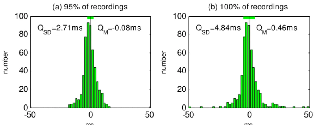
![Table 2. Mean and standard deviations of each referee after the 3rd round Q onset deviations [ms] T end deviations [ms]](https://thumb-eu.123doks.com/thumbv2/123dok_br/18331552.350930/4.892.180.673.584.738/table-mean-standard-deviations-referee-round-deviations-deviations.webp)


Documentos relacionados
At the first stage of the measurements results analysis, the gear wheel cast surface image was compared with the casting mould 3D-CAD model (fig.. Next, the measurements results
The structure of the remelting zone of the steel C90 steel be- fore conventional tempering consitute cells, dendritic cells, sur- rounded with the cementite, inside of
social assistance. The protection of jobs within some enterprises, cooperatives, forms of economical associations, constitute an efficient social policy, totally different from
The probability of attending school four our group of interest in this region increased by 6.5 percentage points after the expansion of the Bolsa Família program in 2007 and
Interval of variation of inbreeding depression (DE) in %, standard deviation and number of progenies with positive and negative DE among the open pollination and
From the cylinder compression test and by performing a linear regression with the data of stress and deformation, the value of the real modulus of elasticity of
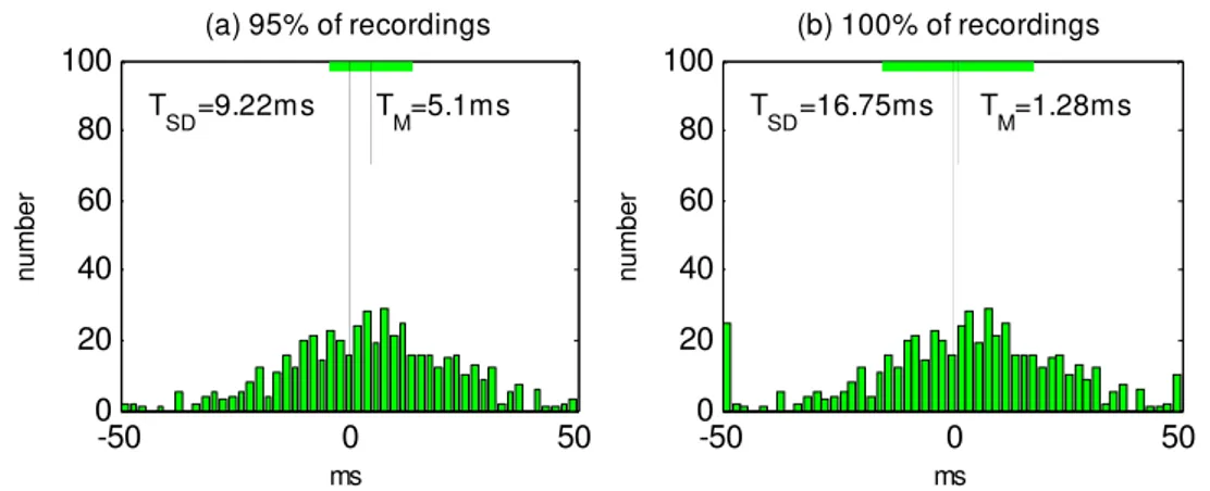
The largest value of the mean distance, the minimum mean distance, the max- imum and minimum standard deviations as a function of the time windows T 1 , T 2 and time lags are
2D descriptors which Fishers’ weight value are above 95% of conidence interval (mean plus two times the standard deviation) (0.497) were selected, gathered,
