A New Method for Re-Analyzing Evaluation
Bias: Piecewise Growth Curve Modeling
Reveals an Asymmetry in the Evaluation of
Pro and Con Arguments
Jens Jirschitzka1, Joachim Kimmerle1,2*, Ulrike Cress1,2
1Leibniz-Institut für Wissensmedien, Tübingen, Germany,2Department of Psychology, Eberhard Karls University of Tübingen, Tübingen, Germany
*j.kimmerle@iwm-tuebingen.de
Abstract
In four studies we tested a new methodological approach to the investigation ofevaluation bias. The usage ofpiecewise growth curve modelingallowed for investigation into the
impact of people’s attitudes on their persuasiveness ratings of pro- and con-arguments,
measured over the whole range of the arguments’polarity from an extreme con to an
extreme pro position. Moreover, this method provided the opportunity to test specific hypotheses about the course of the evaluation bias within certain polarity ranges. We con-ducted two field studies with users of an existing online information portal (Studies 1a and 2a) as participants, and two Internet laboratory studies with mostly student participants (Studies 1b and 2b). In each of these studies we presented pro- and con-arguments, either for the topic of MOOCs (massive open online courses, Studies 1a and 1b) or for the topic of
M-learning (mobile learning, Studies 2a and 2b). Our results indicate that using piecewise
growth curve models is more appropriate than simpler approaches. An important finding of our studies was an asymmetry of the evaluation bias toward pro- or con-arguments: the evaluation bias appeared over the whole polarity range of pro-arguments and increased with more and more extreme polarity. This clear-cut result pattern appeared only on the pro-argument side. For the con-pro-arguments, in contrast, the evaluation bias did not feature such a systematic picture.
Introduction and Theoretical Background
At least since Leon Festinger’s“theory of cognitive dissonance”[1] and Sherif and Hovland’s (1961)“social judgment theory”[2] it is a well-known phenomenon that individuals’prior atti-tudes and beliefs strongly influence how they deal with information and its sources. This is par-ticularly the case if a controversial issue is highly relevant to the recipient and comes along with high affective involvement (e.g., [3–5]). Two kinds of consequences are of particular importance with regard to the impact of prior attitudes and beliefs: (a) selective seeking of
OPEN ACCESS
Citation:Jirschitzka J, Kimmerle J, Cress U (2016) A New Method for Re-Analyzing Evaluation Bias: Piecewise Growth Curve Modeling Reveals an Asymmetry in the Evaluation of Pro and Con Arguments. PLoS ONE 11(2): e0148283. doi:10.1371/journal.pone.0148283
Editor:Delphine S. Courvoisier, University of Geneva, SWITZERLAND
Received:October 15, 2015
Accepted:January 16, 2016
Published:February 3, 2016
Copyright:© 2016 Jirschitzka et al. This is an open access article distributed under the terms of the Creative Commons Attribution License, which permits unrestricted use, distribution, and reproduction in any medium, provided the original author and source are credited.
Data Availability Statement:All relevant data are within the paper and its Supporting Information files.
attitude-consistent information while avoiding attitude-inconsistent information, and (b) over-valuing of attitude-consistent information while deover-valuing or even rejecting attitude-inconsis-tent information (e.g., [6]). While the most suitable term for the former consequences seems to beselective exposure bias(e.g., [7]), the most appropriate term for the latter seems to be evalua-tion bias(e.g., [8–9]).
Other common terms which refer in one sense or another to these phenomena ofmotivated reasoning[10] are:biased assimilation[2,11–12],boomerang/contrast effects [2,13], confirma-tion bias[14–15],congeniality bias[3],disconfirmation bias[6,16],myside bias[17–18], parti-san bias[6,19], andprior attitude/belief effect[6,16]. For reasons of clarity, we will use the termevaluation biashere for referring to the influence ofattitudinal effectson ratings of the arguments in which we were interested.
The attitudinal evaluation bias as well as the selective exposure bias are highly relevant for advertising and health prevention campaigns (e.g., [1,20–21]), socio-political issues (e.g., [6,
22]), and determining media effects (e.g., [23–24]). In this sense, Druckman and Bolsen [22] concluded that“once individuals form initial opinions, they do not‘objectively’incorporate new factual information in ways often assumed by scientific literacy approaches”(p. 681). Moreover, in the current era of Web 2.0, selective exposure to attitude-consistent information and the devaluing of attitude-inconsistent information are frequently observable phenomena in online information searches, news consumption behavior, online forum discussions and vot-ing on comments (e.g., [15,25–27]).
In short, the more or less explicit underlying expectations of the corresponding studies were that people (a) search for attitude-consistent information and avoid attitude-inconsistent information and (b) evaluate attitude-consistent information considerably more favorably and accept it more frequently than attitude-inconsistent information. For example, Lord, Ross and Lepper [11] have shown that both proponents and opponents of the death penalty rated an atti-tude-supportive study (pro-attitudinal information) to be more convincing and more valid than an attitude-disconfirming study (con-attitudinal information). Another example is the also often cited work of Taber and Lodge [6], who found that pro-attitudinal arguments for affirmative action and gun control were rated as stronger than con-attitudinal information, regardless of whether the individuals’prior attitudes were against or in favor of the measure in question.
In most of these studies, however, not only were the participants classified into proponent and opponent groups, but the arguments were also often dichotomized in pro- and con-argu-ments, even when it is intuitively obvious that attitudes as well as the degree of extremeness of pro- and con-arguments (theirpolarity) are more continuous rather than categorical variables. Such dichotomizing strategies may be appropriate in the early stages of research in a given field (e.g., [28]). But the dichotomizing of continuous variables (e.g., by median split) or compari-sons of extreme groups (e.g., the lower against the upper quantile) is not only problematic from a statistical point of view [29–30], but also from a theoretical perspective. Such dichoto-mizing precludes important theoretical insights, as the following remarks illustrate.
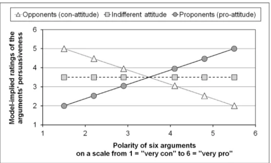
For a hypothetical, controversial issue (e.g., death penalty),Fig 1displays the typical assumption about the ratings of thepersuasivenessof pro- and con-arguments as a function of the participants’prior attitude. AsFig 1indicates, pro-arguments (or con-arguments) are shown to be rated as more persuasive than con-arguments (or pro-arguments) by proponents (or opponents) and vice versa.
If both people’s prior attitudes and the polarity of arguments each are thought to have a continuous metric, however, the question occurs as to what the shapes of the resulting graphs would look like. A plausible answer could be that a pattern of line graphs would result as illus-trated inFig 2, (a) if the persuasiveness ratings are simple monotonic linear functions of the
and analysis, decision to publish, or preparation of the manuscript.
arguments’polarity within each possible attitudinal level (within a range from extreme con to extreme pro), and (b) if the slope of these functions under these conditions is thought to be moderated by participants’attitudes (i.e., an interaction between the predictor variables polar-ityandattitude). For purposes of illustration, we present the three-dimensionality of this hypo-thetical regression surface (polarity and attitude as predictor variables, and persuasiveness ratings as dependent variable). To do this we take three concrete values out of the range of pos-sible values for attitude, although the underlying model should be specified and estimated with
Fig 1. Typical assumption about the average ratings of the persuasiveness of con- and pro-arguments as a function of the prior attitudes of opponents and proponents.
doi:10.1371/journal.pone.0148283.g001
Fig 2. Hypothetical persuasiveness ratings if the continuous metric of arguments’polarity is taken into account.
continuous variables [29]. In the hypothetical example inFig 2, we show the persuasiveness rat-ings of six arguments with differentpolarity scores. As can be seen fromFig 2, the slope for the opponents should be negative (assigning their highest ratings to the most extreme con-argu-ments), whereas the slope of the proponents should be positive (assigning their highest ratings to the most extreme pro-arguments).
This idea has some significant shortcomings, however. First, the variables attitude and polarity are established on two different levels. And second, whereas attitude is a characteristic of individuals (the raters), polarity is a feature of the arguments. Nevertheless, the polarity score of an argument must also be extracted from human ratings, just as in attractiveness research, for example, where physical attractiveness of people must be extracted from the aver-age of several individual ratings, and is treated as a“quasi-objective”characteristic of target persons (e.g., see [31]).
A possible methodological solution to this problem, which we have applied in the present analysis, is to use (piecewise)growth curve modelingthat is (largely) equivalent to certain kinds ofhierarchic linear models(HLM; e.g., see [32–37]). This approach allows for separate inspec-tions of the polarity ranges of con- and pro-arguments, and thus can provide new insights for the research on evaluation bias.
The basic idea is that the persuasiveness ratings ofmarguments can be specified as a repeated measure design withmtime-points. An appropriate method for dealing with these kinds of data isgrowth curve modelingthat allows for specifying linear and nonlinear trends over time whereby graphically the x-axis with the polarity variable represents a predictor con-tinuum at awithin-level(each individual rated the persuasiveness of several arguments with different polarity scores). For this within-level, growth curve models assume that each ual has his/her own growth curve with individual-specific regression parameters (e.g., individ-ual intercepts and slopes for a linear regression of the persuasiveness ratings on polarity). As a consequence, each within-level regression parameter is a random variable with a mean and a variance. Further, on abetween-level, such models allow for specifying these regression param-eters as dependent variables (intercepts- and slopes-as-outcome models) [37], making it possible to study influences of some other variables (e.g., personal characteristics like attitude) on the shape of individual growth curves.
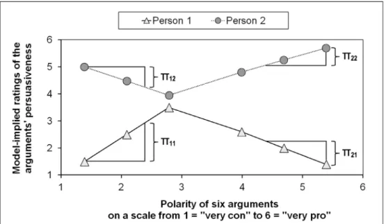
In the present studies, we usedm= 6 arguments (three con- and three pro-arguments), and therefore have six polarity scores on the x-axis (polarity as predictor on the within-level). This allows for splitting the linear growth curves intotwo pieceswith different sizes and signs of the slopes describing separately the region of the three con- and the region of the three pro-argu-ments. So, if the slopes of both regions were in fact different and if the assumption of equal slopes (seeFig 2) does not hold, then such a model with different slopes for the two ranges would be more appropriate for describing individual trajectories.Fig 3illustrates the idea of
piecewise growth curve models(e.g., [32,35,37]) with two fictitious regression lines from two hypothetical individuals, with the ratings of the persuasiveness of six arguments as dependent variables. On the x-axis, the sequence of the arguments begins with the most extreme con-argu-ment (the argucon-argu-ment with the lowest polarity score) and ends with the most extreme pro-argu-ment (the argupro-argu-ment with the highest polarity score). As can be seen inFig 3, hypothetical
person 1has a positive within-level slope for the first three arguments (seeEq 1below, where-upon this slope can be calledπ
11), whereas the within-level slope of hypotheticalperson 2has a
negative value (slopeπ12). The second within-slope for the last three arguments has a negative
value for person 1 (slopeπ21) but a positive value for person 2 (slopeπ22).
scorea.
Yai¼p0iþp1il1aþp2il2aþεai ð1Þ
The deviation of Yaifrom the individual model-implied growth trajectory is represented by
the random effectεai[35,37]. The variablesλ1aandλ2aare two coded variables that contain information about the polarity of an argument with the polarity valuea. Thus, in such a piecewise regression model with two pieces, each polarity scoreais represented by two valuesλ1aandλ2a.
Different coding schemes for two-piece linear models can be found in [37]. In our study, the first scheme in ([37], p. 179) was applied. For illustration purposes, let us assume that there are six hypothetic polarity scores with the values of 1, 2, 3, 4, 5, and 6. The first step in this coding scheme is an additive transformation of the polarity scores, achieved by subtracting the first value from each value in order to set the first score to the value of zero. Thus, the resulting polarity scores would be 0, 1, 2, 3, 4, and 5. To represent these scores with the coding scheme described in [37], the parameterλ2afor the pro-arguments would receive the value of zero for
the first three con-arguments (λ20= 0,λ21= 0, andλ22= 0), and therefore would not play a role for the three con arguments. The parameterλ1awould receive the first three
(difference-trans-formed) polarity scores for its first three values (λ10= 0,λ11= 1, andλ12= 2), would be fixed at the third polarity score for its last three values (λ13= 2,λ14= 2, andλ15= 2), and therefore
would not play a role for the three pro arguments. The parameterλ2awould receive the differ-ences between the last three polarity scores (3, 4, and 5) and the third polarity score (2) for its last three values (λ23= 1,λ24= 2, andλ25= 3). So in our example, the values forλ1awould be 0, 1, 2, 2, 2, and 2, and the values forλ2awould be 0, 0, 0, 1, 2, and 3. If we insert these values into
Eq 1to estimate Yaifor each of the six polarity scores, we would obtain for the first three
polar-ity scores:π0i,π0i+π1i, andπ0i+π1i2. For the last three polarity scores we would obtain:π0i+ π1i2 +π2i,π0i+π1i2 +π2i2, andπ0i+π1i2 +π2i3 (see [37], p. 178–179).
As a consequence of this coding scheme, the parameterπ1iis the individual slope for the
con-arguments, andπ2iis the individual slope for the pro-arguments. The interceptπ0ican be Fig 3. Hypothetical growth curves of two individuals.Individual slopes are labeled withπ11,π12,π21, and π22.
interpreted as an expected persuasiveness rating, if bothλ1aandλ2atake a value of zero (with
the coding scheme applied here, this holds for the most extreme con-argument), and if the pre-dictor variable (attitude) on the between-level also takes a value of zero (see Eqs2–4). If this value has no practical meaning, it is necessary to center the predictor before the analysis (e.g., see [29]).
Sinceπ0i,π1i, andπ2iare random variables that vary among individuals, they can be
explained by another person variable Z (e.g., attitude) on the between-level. This is expressed in Eqs2–4, whereby the interceptsβ00,β10, andβ20as well as the slopesβ01,β11, andβ21in these formulas are fixed effects, while the individual deviationsz0i,z1i, andz2iof the individual
growth parameters from the predicted growth parameters are random effects [35,37].
p0i¼b00þb01Ziþz0i ð2Þ
p1i¼b10þb11Ziþz1i ð3Þ
p2i¼b20þb21Ziþz2i ð4Þ
Eq 5results from inserting Eqs2–4intoEq 1and restructuring accordingly. InEq 5, the term (β01+β11λ1a+β21λ2a) represents the effect of predictor Z on the persuasiveness ratings for polarity scorea. With regard to attitude as predictor Z, this term and its values represent a measure for the size and direction of anattitudinal evaluation biasat a certain polarity scorea.
Yai ¼ ðb00þb10l1aþb20l2aÞ þ ðb01þb11l1aþb21l2aÞ Ziþ ðz0iþz1il1aþz2il2a
þε
iaÞ ð5Þ
Important assumptions that go along with Eqs1–4are (a) that on the within-level, each individual regression of the persuasiveness ratings on thefirst three argument scores as well as the regression on the last three argument scores are linear and (b) that on the between-level, the regressions of the interceptπ0iand the slopesπ1iandπ2ion the predictor Z are also linear.
Theoretically, with enough arguments and their scores, it would also be possible to specify polynomial models on the within-level tofit individual growth curves and to specify higher order regressions for growth parameters on the between-level [37]. However, the correspond-ing results are harder to construe, as Bollen and Curran [32] point out:“higher-order polyno-mial trajectory models become increasingly difficult to interpret when relating model results back to theory”(p. 97). Additionally, it seems intuitively plausible to use a linear piecewise model that splits the whole regression line into two pieces: one for the con-arguments and another piece for the pro-arguments. Moreover, such a piecewise model with two slopes is already much moreflexible than the linear growth curve model with only one slope which is so often used.
Hypotheses
From the remarks above and especially from the theoretical and methodical considerations that are presented graphically in Figs2and3, we derive the following hypotheses about the influence ofattitudeon the evaluation of thepersuasivenessof pro- and con-arguments with different degrees of extremeness (polarity):
Hypothesis H-1
pro-arguments inEq 1; seeFig 3) than with a model that has only one slope (seeFig 2). That means that the within-level slopesπ1iandπ2ishould not be the same (as inFig 3). Therefore, either
the between-level interceptsβ10andβ20, or the between-level slopesβ11andβ21(Eqs3and4),
or both should not have the same values (β10andβ20are unequal and/orβ11andβ21are unequal).
Hypothesis H-2
The evaluation bias should show negative values for all three con-arguments (H-2a for the most extreme con-argument“- - -”, H-2b for the moderately extreme con-argument“- -”and H-2c for the lowest extreme con-argument“-”) and positive values for all three pro-arguments (H-2d for the most extreme pro-argument“+”, H-2e for the moderately extreme pro-argument
“++”and H-2f for the lowest extreme pro-argument“+++”). As an influence of attitude on the persuasiveness ratings for any given argument, the evaluation bias for that given argument is represented by the value of the term (β01+β11λ1a+β21λ2a) inEq 5.
Hypothesis H-3
For con-arguments, the evaluation bias should be strongest for the most extreme con-argument and lowest for the lowest extreme con-argument. That is, the evaluation bias of the most extreme con-argument should be higher (in absolute value) than the bias of the moderately extreme con-argument (H-3a) and higher than the bias of the lowest extreme con-argument (H-3b). The evaluation bias of the moderately extreme con-argument should be higher than the bias of the lowest extreme con-argument (H-3c). An analogous pattern should hold for the pro-arguments. The evaluation bias of the most extreme pro-argument should be higher than the bias of the moderately extreme pro-argument (H-3d) and higher than the bias of the lowest extreme pro-argument (H-3e). The evaluation bias of the moderately extreme pro-argument should be higher than the bias of the lowest extreme pro-argument (H-3f).
Further, and in a cross-validating sense, the hypotheses above should be valid fordifferent topics. Additionally, the expected result patterns should hold for different subgroups of people who may have different perspectives on the topics in question.
Materials and Methods
With two topics, MOOCs (massive open online courses, Study 1) and M-learning (mobile learn-ing, Study 2), we ran two studies, each considering two different participant groups. Partici-pants in the first group were regular users who navigated an existing web information portal and came across the presented material in field studies (Studies 1a and 2a). Participants from the second group were mostly university students who were invited to participate in online studies in order to navigate the same material (Studies 1b and 2b). So the first group represents an existing, ecological valid sample of information searchers on the Web, whereas the second sample encountered the information in a more controlled online laboratory setting.
Participants
lecturers who use digital media for teaching in higher education. Because the portal in 2014 fea-tured specials about MOOCs and M-learning, we used these topics as study material in two consecutive studies (Study 1a and Study 2a). Both topics are controversially discussed. So we could expect them to cause the kind of evaluation biases we aimed to analyze. For the sample of portal users we integrated an informed consent form into the website. When users came across the relevant iframe they were informed that we would use these pages for scientific anal-ysis purposes and that they could leave these sites whenever they wanted to.
We recruited the second group of participants (Studies 1b and 2b) with an online recruit-ment system that is regularly used in our institute to invite people (primarily university stu-dents) to be participants in empirical studies. In the invitation e-mail we did not tell them about the specific content or nature of the study. These participants had to navigate the same portal-like pages with the same material used in Studies 1a and 2a. Thus, Study 1b provided information about MOOCs and Study 2b dealt with information about M-learning. As a com-pensation for their participation, participants in Studies 1b and 2b could enter a lottery where 10 participants had the opportunity to win 20 Euros each.
In addition to the participants described below, some individuals with missing data on all six dependent variables (see below) were not included in the following analyses. From initially
n= 545 participants who visited at least the first page with informed consent content, the sam-ple which remained containsn= 349 individuals who visited the online questionnaireand
rated at least one of the six arguments (one participant had to be excluded because s/he wished to withdraw her/his data). The data file for the main analyses is given inS1 File.
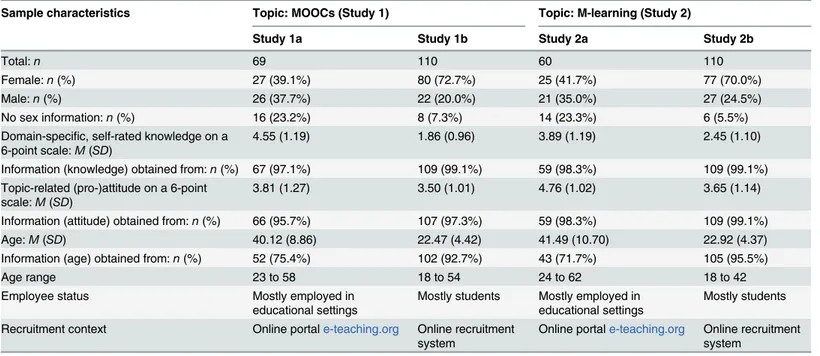
Given the sample of portal users and the natural setting of their participation, however, we cannot be sure whether these people constituted two entirely disjunctive samples in Study 1a and Study 2a (it is possible that some individuals participated in both studies). The samples in Study 1b and Study 2b were entirely disjunctive, however.Table 1summarizes information about sample size, sex ratio, domain-specific knowledge, attitude, and some other characteris-tics of the four groups of participants.
Table 1. Sample description: Participants who rated at least one argument.
Sample characteristics Topic: MOOCs (Study 1) Topic: M-learning (Study 2)
Study 1a Study 1b Study 2a Study 2b
Total:n 69 110 60 110
Female:n(%) 27 (39.1%) 80 (72.7%) 25 (41.7%) 77 (70.0%)
Male:n(%) 26 (37.7%) 22 (20.0%) 21 (35.0%) 27 (24.5%)
No sex information:n(%) 16 (23.2%) 8 (7.3%) 14 (23.3%) 6 (5.5%)
Domain-specific, self-rated knowledge on a 6-point scale:M(SD)
4.55 (1.19) 1.86 (0.96) 3.89 (1.19) 2.45 (1.10)
Information (knowledge) obtained from:n(%) 67 (97.1%) 109 (99.1%) 59 (98.3%) 109 (99.1%) Topic-related (pro-)attitude on a 6-point
scale:M(SD) 3.81 (1.27) 3.50 (1.01) 4.76 (1.02) 3.65 (1.14)
Information (attitude) obtained from:n(%) 66 (95.7%) 107 (97.3%) 59 (98.3%) 109 (99.1%)
Age:M(SD) 40.12 (8.86) 22.47 (4.42) 41.49 (10.70) 22.92 (4.37)
Information (age) obtained from:n(%) 52 (75.4%) 102 (92.7%) 43 (71.7%) 105 (95.5%)
Age range 23 to 58 18 to 54 24 to 62 18 to 42
Employee status Mostly employed in
educational settings Mostly students Mostly employed ineducational settings Mostly students Recruitment context Online portale-teaching.org Online recruitment
Regarding the employee-status, 50 (72.5%) participants in Study 1a and 46 (76.7%) partici-pants in Study 2a belonged to at least one of the following groups: middle or high school teach-ers, college lecturteach-ers, lecturers in continuing or adult education, researchers in academic and non-academic fields, other employees in university institutions, employees in business compa-nies, and self-employed individuals. Ninety-three (84.5%) participants in Study 1b and 100 (90.9%) participants in Study 2b indicated that they were university students.
Material and Pilot Studies
For the topic of MOOCs (Study 1) as well as for the topic of M-learning (Study 2), six arguments were presented on the computer screen with six corresponding buttons, arranged in a horizontal line, and labeled in German language with“open the argument”. Below these buttons was a line with minuses and pluses standing for the polarity of the argument:“- - -”(most extreme con-argument),“- -”,“-”,“+”,“++”,“+++”(most extreme pro-argument). At its ends, the scale was also labeled with the words“contra”and“pro”. The buttons for the con-arguments and the cor-responding region of the line below them were colored in red and the pro-arguments as well as the region of the line below them were colored in green. We randomly assigned the placement of the presented arguments on the screen (“- - -”to“+++”from left to right or from right to left) in order to control for order effects. We also randomly varied the degree of the intensity of the color: in a dichotomized manner or in a more continuous rainbow-like manner. For the focus here and the corresponding variables of interest, these efforts were not relevant, however, even with regard to potential effects and interactions, which were not found to be substantial.
The M-learning arguments were constructed from discussion points which were typical for this topic, whereas the MOOC arguments were taken mainly from a position paper on MOOCs from the German Rectors’Conference [38]. Each argument was in the German language and consisted of either 43 words (MOOC arguments in Studies 1a and 1b) or 44 words (M-learning arguments in Studies 2a and 2b). In order to select appropriate arguments, we conducted two pilot studies where experts (n= 7 for MOOCs andn= 9 for M-learning) rated the polarity and persuasiveness of 37 MOOC and 24 M-learning arguments using six-point rating scales. Inter-rater agreement was estimated with the one-way random single measures intraclass correlation ICC(1,1) [39] (for a missing-tolerant approach, see [40]) and can be considered to be good, ICC (1,1) = .68 for MOOC arguments and ICC(1,1) = .64 for M-learning arguments (for the corre-sponding classification, see [41]). For the final experiments we chose six arguments such that each (a) could be ordered on a con-pro continuum, for which (b) the corresponding inter-rater reliability was comparatively high (indicated by the variance and the agreement score per argu-ment; e.g., see [42]), and for which (c) the persuasiveness scores were on approximately the same level. We also took care to choose arguments which were suitable with regard to content for pre-senting them in the Internet portal we used. The polarity scores (average over the expert raters; e.g., see [43]) of the six selected MOOC arguments were: 1.86, 2.33, 3.17, 4.57, 4.86, and 5.29. Therefore, after applying the coding scheme for piecewise regression models as described in [37] and outlined above, the resulting values forλ1awere 0.00, 0.48, 1.31, 1.31, 1.31, and 1.31 and the resulting values forλ2awere 0.00, 0.00, 0.00, 1.40, 1.69, and 2.12 (seeS2 Filefor more decimal
places). The polarity scores of the six selected M-learning arguments were: 2.11, 2.33, 2.75, 4.67, 5.00, and 5.33. The resulting values forλ1a, after applying the coding scheme, were 0.00, 0.22,
0.64, 0.64, 0.64, and 0.64 and the resulting values forλ2awere 0.00, 0.00, 0.00, 1.92, 2.25, and 2.58. Here is an example for the most extreme con-MOOC argument and an example for the most extreme pro-MOOC argument:
students will no longer be required to read, to understand, or to transfer complex and compre-hensive material.”(con-argument- -).
“Interdisciplinarity and transdisciplinarity are often outspoken ideal wishes for research projects and courses, but these wishes are realized to a lesser extent than is desired. MOOCs can fulfill these claims. Moreover, they can contribute to extending the range of the lecture series’classical university format on a global scale.”(pro-argument +++).
Control Variables, Predictor, and Dependent Variables
At the beginning of our studies, we asked the participants about theirself-rated knowledge
about MOOCs or M-learning respectively (e.g.,“I would guess that my knowledge about MOOCs is relatively high”) with three six-point Likert-scale items (1 =not at all true, 6 =
completely true), whereby one item was inversely worded. The internal consistency (Cronbach’s alpha) for this scale wasα= .87 (MOOCs) andα= .76 (M-learning) respectively. Theattitude
about the topic was also measured with three six-point Likert-scale items (e.g.,“MOOCs should become an important part of university education”, 1 =not at all true6 =completely true), whereby one item was inversely worded. The internal consistency (Cronbach’s alpha) for this scale wasα= .77 (MOOCs) andα= .87 (M-learning) respectively.
The dependent variable was the perceived persuasiveness for each of the six arguments. Each argument was presented together with a six-point one-item rating scale (1 =not at all convincing, 6 =very convincing). If an argument was opened and was rated more than once, the evaluations of this participant were averaged for this argument. We also tracked the navigation behavior of the users to control for the order in which the arguments were opened.
Procedure
Our studies were conducted with approval from the institutional ethics committee of the Leib-niz-Institut für Wissensmedien (Tübingen, Germany; approval numbers: LEK 2014/022, LEK 2014/023, LEK 2014/037, LEK 2014/038, and LEK 2014/039). Participants gave their written informed consent. After that, a website opened asking for participants’topic-relevant knowl-edge about and attitude toward MOOCs or M-learning respectively. Then, six buttons to open each of the six arguments separately appeared on the screen. The buttons could be activated without any coercion to begin with a particular argument. Altogether, the buttons could be clicked a total of seven times, regardless of which button had been opened previously (so an argument could be opened twice or more). There was also the option not to open any argu-ment. After participants clicked on a button, the corresponding argument appeared. It is wor-thy to note that with 299 out of 349 participants (85.7%), a great majority began reading the argument on the left-hand side, regardless of whether the first argument was the most extreme con- or the most extreme pro-argument. This was probably due to the fact that the customary reading direction is from left to right. It was possible for participants to read every argument and rate its perceived persuasiveness. Whether an argument was rated or not, the text could be closed and another text could be opened, or the same text could be opened again.
descriptive results of the study (e.g., ratings of the arguments) were introduced on the website and via newsletters.
Data Analysis Methodology
Estimates of the piecewise growth curve models were done with Mplus 7.3 [44]. The Mplus syntax is given inS2 File. Instead of using the Maximum Likelihood estimator, we applied
Bayesian estimation[45–47]. Among others, important advantages of Bayesian estimation are (a) that it can be used even with small sample sizes, (b) non-normality can be handled better, and (c) estimations of implausible values (e.g., negative variances) are impossible [46–47]. Missing data were appropriately dealt with by the Bayes full-information estimator under the assumption of MAR (missing at random) [48–49].
In the following Bayesian growth curve analyses, non-informative priors were used for the Bayesian estimation procedure and the medians of the posterior distributions were used as point estimates [46–47]. The posterior distributions for the parameters were estimated with the Markov chain Monte Carlo (MCMC) Gibbs sampler algorithm (e.g., see [46,50–51]). For each model, two MCMC chains were used. The convergence criterion was repeatedly assessed (each time after 100 iterations; e.g., see [50]) on the basis of the final half of all iterations per chain. If the criterion was reached, the first half of all iterations from both chains were dropped (burn-in phase) and the posterior distributions were built from the remaining post-burn-in iterations (e.g., see [44,50]). Taking the burn-in phase and the post-burn-in phase together, we specified 30,000 as a minimum and 200,000 as a maximum for the total number of iterations per chain.
For determining the convergence, we used the Gelman-Rubin convergence criterion [44,
52]. Convergence is reached when the Potential scale reduction (PSR; see [53]) is smaller than: a = 1 + bc, where c is 2 for a large number of parameters in the model (see [44], p. 634). Thus, because we set b to the value of 0.001, the PSR had to be smaller than 1.002. This is a very strict criterion, since the PSR should be very close to 1.00, and values of 1.05 already indicate a good convergence (e.g., see [46–47,50]).
With Bayesian estimation, credibility intervals (not necessesarily symmetric) are produced for estimated parameters about which statements can be made; for instance, that there is“a 95% probability that the population value is within the limits of the interval”([46], p. 844, see also [54–56]). If the value zero does not lie within this interval, the result can be interpreted as significant according to classical frequentist null hypothesis testing [46]. However, the essential focus of Bayesian analyses is not on conditional probabilities of the data given certain (null) hypotheses, as in the frequentist approach, but on posterior conditional probabilities of hypotheses given the data (e.g., see [54–56]). Although this is the case, we still address the mul-tiple testing problem, that is, the overall risk of false significance alarms which increases with the number of conducted significance tests (e.g., see [57–58]), by using more conservative 99% credibility intervals instead of 95% credibility intervals for the posterior distributions. Model comparisons (e.g., a model with parameter constraints vs. a model with freely estimated parameters) were made with thedeviance information criterion(DIC; [59]), whereby from two competing models the model with the smaller DIC should be chosen as the better model (e.g., see [51,60–61]).
Results
Piecewise Growth Curve Models
The following analyses consisted of two multi-group piecewise growth curve models with freely estimated within-level and between-level parameters: (a) one separate multi-group model for the MOOC topic and (b) one multi-group model for the topic of M-learning. The measured attitude toward the corresponding topic served as between-level predictor. For model estima-tion, the polarity value for the most extreme con-argument was fixed to the value of zero, which implies a difference transformation of the polarity values of all six arguments. The atti-tude variable was centered at the theoretical midpoint of the scale (3.5).
The first model (MOOC topic) converged after 71,700 iterations (PSR<1.002). Therefore,
the final 35,850 iterations from each of the two chains were used to build the posterior distribu-tions (post-burn-in phase). The second model (M-learning) converged after 40,400 iteradistribu-tions (PSR<1.002), so the final 20,200 iterations from each of the two chains were used to build the
posterior distributions.
The group-specific between-level parameters for the prediction of the within-level parame-ters from attitude are displayed inS1,S2, andS3Tables. The significance of the parameters regarding the value of zero can be concluded from the Bayesian 99% credibility interval for each parameter. If an interval does not contain the value of zero, the estimated parameter can be regarded as significant.
To illustrate the results graphically, for each topic and separately for each group of partici-pants, within-level parameters (π0i,π1i,π2i) of the growth curves within each group were
pre-dicted (a) from attitude values that were one group-specific standard deviation below the group mean of the midpoint-centered attitude variable, (b) from values that resembled the atti-tude group mean of the midpoint-centered attiatti-tude variable, and (c) from values that were one group-specific standard deviation above the group mean.Fig 4shows these curves for the MOOC topic (Studies 1a and 1b) andFig 5for the M-learning topic (Studies 2a and 2b). For purposes of simplification with regard to Figs4and5, the polarity values of the arguments on the x-axis were back-transformed to the original values which were taken from the two pilot studies.
As most of the graphs in Figs4and5indicate, only the slopes for the pro-arguments were influenced by attitude, whereby stronger pro-attitudes came along with comparably steeper positive slopes for the individual trajectories at the polarity-range of the pro-arguments. At the same time, con-attitudes went hand in hand with negative slopes. In other words, increases in the extremeness of pro-arguments led to increases of differences in the persuasiveness ratings between individuals with pro-attitudes and individuals with con-attitudes. This phenomenon is asymmetrical, as it seems to be the case only with pro-arguments. For con-arguments, poten-tial attitude-dependent differences in the persuasiveness ratings remained rather stable, regard-less of the extremeness of the con-arguments.
This result pattern was also represented in the size and significance of the between-level slopes (seeS2andS3Tables). For the prediction of the within-level slope for the con-argu-ments (π1i), there was no significant effect of attitude (seeS2 Table). With regard to the
within-level slope for the pro-arguments (π2i), however, in three of the four groups we found a
signifi-cant positive effect of attitude (seeS3 Table). This means that the shape of the first part of the individual piecewise trajectories (the persuasiveness ratings of the three con-arguments) was not affected by the attitude toward the topic. However, the shape of the second part of the indi-vidual piecewise trajectories (the persuasiveness ratings of the three pro-arguments) was affected by the attitude in such a way that the stronger the attitude, the higher was the slope of this second part of the trajectories; and the weaker the attitude, the lower (or more negative) was the slope of this second piece. Even though there was no significant effect of attitude onπ
in the M-learning group of portal users (Study 2a), it is remarkable that also this parameter has a positive sign (seeS3 Table).
Hypothesis H-1
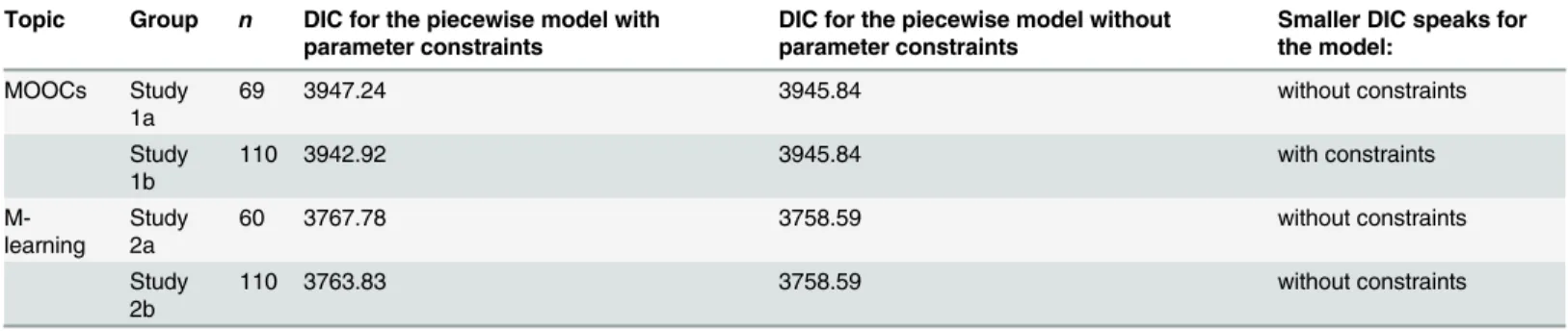
To be able to determine whether using a (bi-linear) piecewise growth curve model was more appropriate than just using a linear growth curve model with only one single within-level slope for the whole polarity range from con to pro (as inFig 2), both models were compared in each study with the help of thedeviance information criterion(DIC). The model with the smaller DIC would be regarded as the better model. The simple linear growth curve models had the specification that the between-level interceptsβ10andβ20as well as the between-level slopes
β11andβ21were held equal. The results for all four studies are shown inTable 2.
As can be concluded fromTable 2, for three of the four studies, a (bi-linear) piecewise model was shown to be to be more appropriate than a simple growth curve model with only one slope. Thus, three of the four studies support H-1.
Fig 5. Piecewise growth curves: M-learning.(A) Study 2a. (B) Study 2b. doi:10.1371/journal.pone.0148283.g005
Table 2. Model comparisons (model with parameter constraints:β10andβ20as well asβ11andβ21are held equal) with the deviance information
criterion (DIC).
Topic Group n DIC for the piecewise model with parameter constraints
DIC for the piecewise model without parameter constraints
Smaller DIC speaks for the model:
MOOCs Study
1a 69 3947.24 3945.84 without constraints
Study
1b 110 3942.92 3945.84 with constraints
M-learning Study2a 60 3767.78 3758.59 without constraints
Study
2b 110 3763.83 3758.59 without constraints
Hypothesis H-2
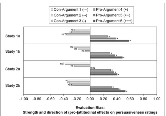
The sign, size, and significance of the influence of attitude on the persuasiveness ratings ( attitu-dinal evaluation bias; seeEq 5) for each argument are depicted inFig 6for all four studies. The corresponding numerical results are given inS4andS5Tables.
On the basis of this result pattern, we conclude that hypotheses H-2d (for argument“+”), H-2e (“++”) and H-2f (“+++”) for significant and positive evaluation biases toward the pro-argumentscan be maintained within all four studies. For the con-arguments, hypothesis H-2a (“- - -”) can be maintained only in Study 2b and must be rejected for Studies 1a, 1b, and 2a. Hypothesis H-2b (“- -”) can be maintained only in Studies 1a and 2b and must be rejected for Studies 1b and 2a. Hypothesis H-2c (“-”) must be rejected within all four studies.
Hypothesis H-3
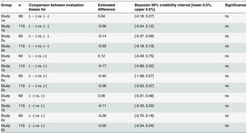
In the final step, we compared evaluation biases of all three con- and all three pro-arguments with each other, for each kind of argument.Table 3shows the results of these comparisons for the con-arguments. AsTable 3indicates, for the con-arguments the postulated pairwise differ-ences with regard to the evaluation bias magnitude were not significant in all four studies. That is, there were no significant differences and seemingly no covariation of the evaluation bias with the polarity extremeness of the con-arguments.
For the pro-arguments, in contrast, the postulated significant pairwise differences can be found in three of the four studies (seeTable 4). That is, in three of the four studies, there was a covariation of the evaluation bias with the polarity extremeness of the pro-arguments.
Fig 6. Attitudinal evaluation bias: Sign, size, and significance of the influence of attitude on the persuasiveness ratings for each argument for each of the four studies.(*) Bayesian 99% credibility
interval for evaluation bias does not contain the value of zero (significant). (ns) Bayesian 99% credibility interval contains the value of zero (not significant). (†) A 95% credibility interval would not contain the value of zero.
Altogether, the hypotheses H-3a, H-3b, and H-3c about evaluation bias differences between the three con-arguments must be rejected in all four studies. These results go along with the findings that the influence of attitude on the within-level slope for the con-arguments (first part of individual trajectories) was not significant in any of our studies. In contrast, the hypoth-eses H-3d, H-3e, and H-3f about bias magnitude differences between the three pro-arguments can be maintained in at least three of our four studies. Thus, an appropriate final conclusion seems to be that the evaluation bias magnitude co-varies at the polarity range of the pro-argu-ments (with higher magnitudes for higher polarity values), whereas it seems to be rather stant, or at least without any systematic pattern, over the whole polarity range of the con-arguments.
Discussion and Conclusions
The aim of our study was to explore the evaluation bias over the whole range of pro- and con-arguments, using M-learning and MOOCs as topics for stimulating reactions. For this purpose, the application of (bi-linear) piecewise growth curve modeling seems to be a successful
approach. Moreover, in three of the four studied groups it was more appropriate than using a simple growth curve approach with only one within-level slope for both kinds of arguments. Additionally, this more sophisticated approach allowed for separate inspection of the polarity ranges of pro- and con-arguments.
The results reveal that there were no significant effects of attitude on the within-level slopes for the con-arguments (the first part of the individual trajectories). However, in three of the four groups, significant effects of attitude on the within-level slopes for the pro-arguments appeared (i.e., for the second part of the individual trajectories).
Table 3. Pairwise comparisons between attitudinal evaluation biases within the con-arguments.ns: Bayesian 99% credibility interval contains the value of zero (not significant).
Group n Comparison between evaluation biases for
Estimated difference
Bayesian 99% credibility interval [lower 0.5%, upper 0.5%]
Significance
Study 1a
69 (- - -) vs. (- -) 0.04 [-0.18, 0.27] ns
Study 1b
110 (- - -) vs. (- -) -0.06 [-0.24, 0.12] ns
Study 2a
60 (- - -) vs. (- -) -0.14 [-0.37, 0.09] ns
Study 2b
110 (- - -) vs. (- -) -0.03 [-0.18, 0.13] ns
Study 1a
69 (- - -) vs. (-) 0.12 [-0.49, 0.75] ns
Study 1b
110 (- - -) vs. (-) -0.17 [-0.66, 0.32] ns
Study 2a
60 (- - -) vs. (-) -0.40 [-1.08, 0.27] ns
Study 2b
110 (- - -) vs. (-) -0.08 [-0.53, 0.37] ns
Study 1a
69 (- -) vs. (-) 0.08 [-0.31, 0.48] ns
Study 1b
110 (- -) vs. (-) -0.11 [-0.42, 0.20] ns
Study 2a
60 (- -) vs. (-) -0.26 [-0.70, 0.18] ns
Study 2b
110 (- -) vs. (-) -0.05 [-0.34, 0.24] ns
Inspection of the evaluation bias (the assigning of higher ratings to attitude-consistent and lower ratings to attitude-inconsistent arguments) revealed significant positive attitudinal bias effects on the evaluation of all three pro-arguments in both groups and for both topics. In con-trast, the results for the con-arguments were mixed and less clear. Although mostly negative in its sign, from all evaluation biases that could be estimated for each group, topic, and for each con-argument, only a quarter of these estimates reached significance. Pairwise comparisons of the evaluation biases within the con- and pro-arguments showed that the magnitude of the evaluation bias for the pro-arguments differed between them in three of the four groups. This result resembles the finding that in (the same) three of the four groups a significant effect of attitude on the within-slopes for the pro-arguments were also found. In contrast, no significant bias magnitude differences could be found between the con-arguments.
Altogether, the attitudinal evaluation bias varied in its magnitude within the pro-attitude polarity range (with higher biased ratings at more extreme pro-arguments), whereas the evalu-ation bias seemed to be stable (and/or weak to almost non-existent) for the con-arguments. This observed phenomenon describes anasymmetryin the drift of the evaluation bias over the polarity range of con- and pro-arguments.
This asymmetry did not appear within Study 2a, however. The sample in Study 2a was char-acterized by comparably high favorable attitudes toward M-learning. It is possible that these favorable attitudes resulted in high magnitudes of evaluation bias for a large range of pro-argu-ments’polarity, and that there was little space for the evaluation bias to vary in its (high) mag-nitude from one pro-argument to another. Moreover, it is possible that the people in Study 2a,
Table 4. Pairwise comparisons between attitudinal evaluation biases within the pro-arguments.
Group n Comparison between evaluation biases for
Estimated difference
Bayesian 99% credibility interval [lower 0.5%, upper 0.5%]
Significance
Study
1a 69 (++) vs. (+) 0.13 [0.05, 0.20] *
Study
1b 110 (++) vs. (+) 0.08 [0.02, 0.14] *
Study
2a 60 (++) vs. (+) 0.05 [-0.02, 0.12] ns
Study
2b 110 (++) vs. (+) 0.10 [0.05, 0.16] *
Study
1a 69 (+++) vs. (+) 0.32 [0.13, 0.51] *
Study
1b 110 (+++) vs. (+) 0.19 [0.04, 0.34] *
Study
2a 60 (+++) vs. (+) 0.10 [-0.04, 0.24] ns
Study
2b 110 (+++) vs. (+) 0.20 [0.10, 0.31] *
Study
1a 69 (+++) vs. (++) 0.19 [0.08, 0.30] *
Study
1b 110 (+++) vs. (++) 0.11 [0.02, 0.20] *
Study
2a 60 (+++) vs. (++) 0.05 [-0.02, 0.12] ns
Study
2b 110 (+++) vs. (++) 0.10 [0.05, 0.16] *
*Bayesian 99% credibility interval does not contain the value of zero (significant). ns: Bayesian 99% credibility interval contains the value of zero (not significant).
characterized by relatively high self-rated knowledge as well as by a high favorable attitude toward M-learning, subjectively saw only little polarity differences between the three pro-argu-ments and, as a consequence, they did not differentiate enough between them during the assessment of the pro-arguments.
Regarding external validity, it seems premature to come to the general conclusion that the evaluation bias varies in its magnitude primarily for pro-arguments, even though the question arises as to why such a bias drift was not observable for the con-arguments. It could be that the evaluation of con-arguments required more cognitive effort in general and, as a consequence, there was less space for an evaluation bias to vary with the polarity. Another possibility is that most participants did not realize the con-arguments’polarity or that they did not take these polarity differences into account. Thus, in comparison to pro-arguments, con-arguments were seemingly not differentiated enough with regard to their polarity. It is also possible that the con-arguments did not sufficiently cover the whole range of the polarity scale, although care was taken in the pilot studies to choose only arguments with similar persuasiveness scores and for which the expert ratings resulted in high inter-rater agreement.
For each of these possible explanations, domain- and population-dependencies must be considered. The MOOC and the M-learning topic are future-oriented and rather positively val-ued issues. Hence, in future research, not only other issues but especially more controversial or emotionally charged topics should be examined (e.g., political, religious, or ethnic conflicts). At the moment, we cannot rule out that the asymmetry will eventually disappear for more nega-tive-valued topics. Moreover, it is even imaginable that the direction of the asymmetry might be reversed for more negatively valued topics.
In any case, attention should be paid to the fact that the significance of any issue is always dependent upon its meaning to the particular subpopulation which is studied. The groups in our Studies 1a and 2a had a higher self-rated knowledge than the groups in Studies 1b and 2b, and with regard to the M-learning topic, the group in Study 2a had a comparatively more favorable attitude than the group in Study 2b. Additionally, the proportion of women was much lower and the mean age was much higher in Studies 1a and 2a than in the Studies 2a and 2b. However, even if the group membership was confounded with many third variables, disen-tangling these effects is out of the scope of the present research, but it should be considered in future studies. Nevertheless, with the samples used in the present studies, and especially with regard to the e-teaching community, a much higher degree of ecological validity and potential reproducibility was reached than is possible by using only a homogeneous group of university students dealing with an artificial issue (e.g., see [62]). With regard to the comparatively high self-rated knowledge of the participants in Studies 1a and 2a, it seems clear that even real domain-experts are not immune to evaluation bias in their own domain [63–65]. Taken together, future research should explore for which topics and communities certain effects can be found.
An important limitation of our study has to be noted with regard to the dependent variable. Although the arguments’polarity scores were indeed mean values (averaged over the raters in the pilot studies; e.g., see [66]), the individual persuasiveness ratings of the arguments in the main studies were measured with a single-item rating scale with six ordered categories. The question as to whether and when such rating scales can be treated as interval-scaled variables with regard to the analysis method is an issue which is hotly debated between“purists”and
In this sense, single-item rating scales were successfully used, for example, to measure the subjective convincingness of presented material (e.g., a scale ranging fromcompletely uncon-vincingtocompletely convincing; [11], p. 2101), to measure the participant’s self-rated political ideology (e.g., a scale ranging fromextremely lefttoextremely right; [70], p. 1428; see [71–72]) or to assess the physical attractiveness of target persons (e.g., a scale ranging fromnot attractive
tovery attractive; [43], p. 203; see [42]). The single-item persuasiveness rating-scale in our studies, in which participants should read and judge arguments in an ecologically valid way, was used in the same sense methodologically. Additionally, it must be emphasized that in rare cases, the same argument was opened and rated more than once by the same participant. Such multiple evaluations of the same argument were averaged and accordingly, the corresponding persuasiveness ratings could take on values other than 1, 2, 3, 4, 5, and 6.
However, future studies should replicate our result patterns with persuasiveness scales that consist of a set of several items or by adapting our basic ideas to approaches for categorical out-comes (e.g., [34,73]). Nevertheless, the fact that we could find similar results in four indepen-dent and different samples could be taken as an indication that our findings are indeed substantial and not mere methodological artifacts.
Finally, the usage of the Bayesian estimator provided some advantages; for example, the avoidance of parameter estimates with implausible values, which can result with Maximum-Likelihood estimators [46]. In future research, other advantages of Bayesian methods should be taken into consideration (e.g., the usage of informative instead of non-informative priors; see [46–47]). Additionally, the usage of (two-part) piecewise growth curve modeling seems to be more appropriate than (a) the simple dichotomizing of arguments into two categories and more appropriate than (b) the usage of simple (single-part) growth curve models with only one within-level slope for all arguments. With more arguments, more complex models can allow for more specifications and be tested (e.g., a three-part piecewise growth curve model; see [35,
37]).
Supporting Information
S1 Table. Group-specific between-level parameters for the prediction of the within-level
interceptπ0i.
(PDF)
S2 Table. Group-specific between-level parameters for the prediction of the within-level slopeπ1i.
(PDF)
S3 Table. Group-specific between-level parameters for the prediction of the within-level slopeπ2i.
(PDF)
S4 Table. Group-specific attitudinal evaluation bias for each con-argument.
(PDF)
S5 Table. Group-specific attitudinal evaluation bias for each pro-argument.
(PDF)
S1 File. Data for the main analyses.
(DAT)
S2 File. Mplus syntax.
Acknowledgments
We are grateful to thee-teaching.orgteam for supporting our work.
Author Contributions
Conceived and designed the experiments: JJ JK UC. Performed the experiments: JJ. Analyzed the data: JJ. Contributed reagents/materials/analysis tools: JJ JK UC. Wrote the paper: JJ JK UC. Conceptualized the analysis steps: JJ JK UC. Drafting of the paper: JJ JK UC.
References
1. Festinger L. A theory of cognitive dissonance. 1st ed. Evanston, IL, US: Row, Peterson and Company; 1957.
2. Sherif M, Hovland CI. Yale studies in attitude and communication: Vol. 4. Social judgment: Assimilation and contrast effects in communication and attitude change. 2nd ed. New Haven, CT, US: Yale Univer-sity Press; 1961.
3. Hart W, Albarracín D, Eagly AH, Brechan I, Lindberg MJ, Merrill L. Feeling validated versus being cor-rect: A meta-analysis of selective exposure to information. Psychological Bulletin. 2009 Jul; 135(4): 555–588. doi:10.1037/a0015701PMID:19586162
4. Matthes J. The affective underpinnings of hostile media perceptions: Exploring the distinct effects of affective and cognitive involvement. Communication Research. 2011 Jun; 40(3): 360–387.
5. Nickerson RS. Confirmation bias: A ubiquitous phenomenon in many guises. Review of General Psy-chology. 1998 Jun; 2(2): 175–220.
6. Taber CS, Lodge M. Motivated skepticism in the evaluation of political beliefs. American Journal of Political Science. 2006 Jul; 50(3): 755–769.
7. Knobloch-Westerwick S, Meng J. Looking the other way: Selective exposure to attitude-consistent and counterattitudinal political information. Communication Research. 2009 Jun; 36(3): 426–448.
8. Mojzisch A, Grouneva L, Schulz-Hardt S. Biased evaluation of information during discussion: Disentan-gling the effects of preference consistency, social validation, and ownership of information. European Journal of Social Psychology. 2010 Oct; 40(6): 946–956.
9. Schwind C, Buder J. Reducing confirmation bias and evaluation bias: When are preference-inconsis-tent recommendations effective–and when not? Computers in Human Behavior. 2012 Nov; 28(6): 2280–2290.
10. Kunda Z. The case for motivated reasoning. Psychological Bulletin. 1990 Nov; 108(3): 480–498. PMID:2270237
11. Lord CG, Ross L, Lepper MR. Biased assimilation and attitude polarization: The effects of prior theories on subsequently considered evidence. Journal of Personality and Social Psychology. 1979 Nov; 37 (11): 2098–2109.
12. Richardson JD, Huddy WP, Morgan SM. The hostile media effect, biased assimilation, and perceptions of a presidential debate. Journal of Applied Social Psychology. 2008 May; 38(5): 1255–1270. 13. Hart PS, Nisbet EC. Boomerang effects in science communication: How motivated reasoning and
iden-tity cues amplify opinion polarization about climate mitigation policies. Communication Research. 2012 Dec; 39(6): 701–723.
14. Jonas E, Schulz-Hardt S, Frey D, Thelen N. Confirmation bias in sequential information search after preliminary decisions: An expansion of dissonance theoretical research on selective exposure to infor-mation. Journal of Personality and Social Psychology. 2001 Apr; 80(4): 557–571. PMID:11316221 15. Schwind C, Buder J, Cress U, Hesse FW. Preference-inconsistent recommendations: An effective
approach for reducing confirmation bias and stimulating divergent thinking? Computers & Education. 2012 Feb; 58(2): 787–796.
16. Edwards K, Smith EE. A disconfirmation bias in the evaluation of arguments. Journal of Personality and Social Psychology. 1996 Jul; 71(1): 5–24.
17. Stanovich KE, West RF. Natural myside bias is independent of cognitive ability. Thinking & Reasoning. 2007 Aug; 13(3): 225–247.
18. Wolfe CR, Britt MA. The locus of the myside bias in written argumentation. Thinking & Reasoning. 2008 Feb; 14(1): 1–27.
20. Bientzle M, Cress U, Kimmerle J. The role of tentative decisions and health concepts in assessing infor-mation about mammography screening. Psychology, Health & Medicine. 2015 Aug; 20(6): 670–679. 21. Perrissol S, Somat A. Do alcohol and tobacco advertisements have an impact on consumption?
Contri-bution of the theory of selective exposure. In: Kiefer KH, editor. Applied psychology research trends. 1st ed. Hauppauge, NY, US: Nova Science Publishers; 2008. pp. 1–34.
22. Druckman JN, Bolsen T. Framing, motivated reasoning, and opinions about emergent technologies. Journal of Communication. 2011 Aug; 61(4): 659–688.
23. Kempf W, Thiel S. On the interaction between media frames and individual frames of the Israeli-Pales-tinian conflict. conflict & communication online. 2012; 11(2). [open access journal: copyright by verlag irena regener berlin–creative commons licence: BY-NC-ND]. Available:http://www.cco.regener-online. de/2012_2/pdf/kempf-thiel-neu.pdf. Accessed 2 October 2015.
24. Entman RM, Matthes J, Pellicano L. Nature, sources, and effects of news framing. In: Wahl-Jorgensen K, Hanitzsch T, editors. The handbook of journalism studies. 1st ed. New York, NY, US: Routledge; 2009. pp. 175–190.
25. Garrett RK, Stroud NJ. Partisan paths to exposure diversity: Differences in pro‐and counterattitudinal news consumption. Journal of Communication. 2014 Aug; 64(4): 680–701.
26. Kimmerle J, Thiel A, Gerbing KK, Bientzle M, Halatchliyski I, Cress U. Knowledge construction in an outsider community: Extending the communities of practice concept. Computers in Human Behavior. 2013 May; 29(3): 1078–1090.
27. Van Strien JLH, Brand-Gruwel S, Boshuizen HPA. Dealing with conflicting information from multiple nonlinear texts: Effects of prior attitudes. Computers in Human Behavior. 2014 Mar; 32: 101–111. 28. McClelland DC. Motivational configurations. In: Smith CP, editor. Motivation and personality: Handbook
of thematic content analysis. 1st ed. New York, NY, US: Cambridge University Press; 1992. pp. 87– 99.
29. Cohen J, Cohen P, West SG, Aiken LS. Applied multiple regression/correlation analysis for the behav-ioral sciences. 3rd ed. Mahwah, NJ, US: Erlbaum; 2003.
30. MacCallum RC, Zhang S, Preacher KJ, Rucker DD. On the practice of dichotomization of quantitative variables. Psychological Methods. 2002 Mar; 7(1): 19–40. PMID:11928888
31. Hönekopp J, Becker BJ, Oswald FL. The meaning and suitability of various effect sizes for structured rater × ratee designs. Psychological Methods. 2006 Mar; 11(1): 72–86. PMID:16594768
32. Bollen KA, Curran PJ. Latent curve models: A structural equation perspective. 1st ed. Hoboken, NJ, US: Wiley; 2006.
33. Curran PJ, Obeidat K, Losardo D. Twelve frequently asked questions about growth curve modeling. Journal of Cognition and Development. 2010 Apr; 11(2): 121–136. PMID:21743795
34. Duncan TE, Duncan SC, Strycker LA. An introduction to latent growth curve modeling: Concepts, issues, and applications. 2nd ed. Mahwah, NJ, US: Erlbaum; 2006.
35. Holt JK. Modeling growth using multilevel and alternative approaches. In: O’Connell AA, McCoach DB, editors. Multilevel modeling of educational data. 1st ed. Charlotte, NC, US: Information Age Publish-ing; 2008. pp. 111–159.
36. O’Connell AA, McCoach DB, editors. Multilevel modeling of educational data. 1st ed. Charlotte, NC, US: Information Age Publishing; 2008.
37. Raudenbush SW, Bryk AS. Hierarchical linear models: Applications and data analysis methods. 2nd ed. Thousand Oaks, CA, US: Sage; 2002.
38. Hochschulrektorenkonferenz [German Rectors’Conference]. Beiträge zur Hochschulpolitik 2/1014. Potenziale und Probleme von MOOCs: Eine Einordnung im Kontext der digitalen Lehre [Contributions to higher education policy 2/2014. Potentials and problems of MOOCs: An integration in the context of digital teaching]; 2014. Available:http://www.hrk.de/uploads/media/2014-07-17_Endversion_MOOCs. pdf. Accessed 29 September 2015.
39. Shrout PE, Fleiss JL. Intraclass correlations: Uses in assessing rater reliability. Psychological Bulletin. 1979 Mar; 86(2): 420–428. PMID:18839484
40. Gwet KL. Handbook of inter-rater reliability: The definitive guide to measuring the extent of agreement among multiple raters. 3rd ed. Gaithersburg, MD, US: Advanced Analytics, LLC; 2012.
41. Cicchetti DV, Sparrow SS. Developing criteria for establishing interrater reliability of specific items: Applications to assessment of adaptive behavior. American Journal of Mental Deficiency. 1981 Sep; 86(2): 127–137. PMID:7315877
43. Hönekopp J. Once more: Is beauty in the eye of the beholder? Relative contributions of private and shared taste to judgments of facial attractiveness. Journal of Experimental Psychology. 2006 Apr; 32 (2): 199–209. PMID:16634665
44. Muthén LK, Muthén BO. Mplus User’s Guide. 7th ed. Los Angeles, CA, US: Muthén & Muthén; 2012. 45. Muthén B. Bayesian analysis in Mplus: A brief introduction [Manuscript]; 2010. Available:https://www.
statmodel.com/download/IntroBayesVersion%203.pdf. Accessed 12 September 2015.
46. Van de Schoot R, Kaplan D, Denissen J, Asendorpf JB, Neyer FJ, van Aken MAG. A gentle introduction to Bayesian analysis: Applications to developmental research. Child Development. 2014 May-Jun; 85 (3): 842–860. doi:10.1111/cdev.12169PMID:24116396
47. Zyphur MJ, Oswald FL. Bayesian estimation and inference: A user’s guide. Journal of Management. 2015 Feb; 41(2): 390–420.
48. Asparouhov T, Muthén B. Bayesian analysis of latent variable models using Mplus [Manuscript]; 2010. Available:https://www.statmodel.com/download/BayesAdvantages18.pdf. Accessed 12 September 2015.
49. Enders CK. Applied missing data analysis. 1st ed. New York, NY, US: Guilford Press; 2010. 50. Brown TA. Confirmatory factor analysis for applied research. 2nd ed. New York, NY, US: Guilford
Press; 2015.
51. Kaplan D, Depaoli S. Bayesian statistical methods. In: Little TD, editor. The Oxford handbook of quanti-tative methods (Vol. 1). 1st ed. New York, NY, US: Oxford University Press; 2013. pp. 407–437. 52. Gelman A, Rubin DB. Inference from iterative simulation using multiple sequences. Statistical Science.
1992 Nov; 7(4): 457–511.
53. Gelman A, Carlin JB, Stern HS, Dunson DB, Vehtari A, Rubin DB. Bayesian data analysis. 3rd ed. Boca Raton, FL, US: Chapman & Hall/CRC; 2013.
54. Dienes Z. Understanding psychology as a science: An introduction to scientific and statistical inference. 1st ed. Basingstoke, Hampshire, United Kingdom: Palgrave Macmillan; 2008.
55. Dienes Z. Bayesian versus orthodox statistics: Which side are you on? Perspectives on Psychological Science. 2011 May; 6(3): 274–290. doi:10.1177/1745691611406920PMID:26168518
56. Kruschke JK. Doing Bayesian data analysis: A tutorial with R, JAGS, and Stan. 2nd ed. San Diego, CA, US: Academic Press; 2015.
57. Bretz F, Hothorn T, Westfall P. Multiple comparisons using R. 1st ed. Boca Raton, FL, US: Chapman & Hall/CRC; 2010.
58. Shaffer JP. Multiple hypothesis testing. Annual Review of Psychology. 1995; 46: 561–584.
59. Spiegelhalter DJ, Best NG, Carlin BP, van der Linde A. Bayesian measures of model complexity and fit. Journal of the Royal Statistical Society: Series B. 2002; 64(4): 583–639.
60. Asparouhov T, Muthén B. General random effect latent variable modeling: Random subjects, items, contexts, and parameters [Manuscript]; 2014. Available:https://www.statmodel.com/download/NCME_ revision2.pdf. Accessed 12 September 2015.
61. Kaplan D, Depaoli S. Bayesian structural equation modeling. In: Hoyle R, editor. Handbook of structural equation modeling. 1st ed. New York, NY, US: Guilford Press; 2012. pp. 650–673.
62. Peterson RA, Merunka DR. Convenience samples of college students and research reproducibility. Journal of Business Research. 2014 May; 67(5): 1035–1041.
63. Hergovich A, Schott R, Burger C. Biased evaluation of abstracts depending on topic and conclusion: Further evidence of a confirmation bias within scientific psychology. Current Psychology. 2010 Sep; 29 (3): 188–209.
64. Kassin SM, Dror IE, Kukucka J. The forensic confirmation bias: Problems, perspectives, and proposed solutions. Journal of Applied Research in Memory and Cognition. 2013 Mar; 2(1): 42–52.
65. Mendel R, Traut-Mattausch E, Jonas E, Leucht S, Kane JM, Maino K, et al. Confirmation bias: Why psy-chiatrists stick to wrong preliminary diagnoses. Psychological Medicine. 2011 Dec; 41(12): 2651– 2659. doi:10.1017/S0033291711000808PMID:21733217
66. Cunningham MR, Barbee AP, Pike CL. What do women want? Facialmetric assessment of multiple motives in the perception of male facial physical attractiveness. Journal of Personality and Social Psy-chology. 1990 Jul; 59(1): 61–72. PMID:2213490
68. Hassebrauck M. Die Beurteilung der physischen Attraktivität [The assessment of physical attractive-ness]. In: Hassebrauck M, Niketta R, editors. Physische Attraktivität [Physical attractiveattractive-ness]. 1st ed. Göttingen, Germany: Hogrefe; 1993. pp. 29–59.
69. Rhemtulla M, Brosseau-Liard PÉ, Savalei V. When can categorical variables be treated as continuous? A comparison of robust continuous and categorical SEM estimation methods under suboptimal condi-tions. Psychological Methods. 2012 Sep; 17(3): 354–373. doi:10.1037/a0029315PMID:22799625 70. Cohrs JC, Moschner B, Maes J, Kielmann S. The motivational bases of right-wing authoritarianism and
social dominance orientation: Relations to values and attitudes in the aftermath of September 11, 2001. Personality and Social Psychology Bulletin. 2005 Oct; 31(10): 1425–1434. PMID:16143673
71. Dallago F, Cima R, Roccato M, Ricolfi L, Mirisola A. The correlation between right-wing authoritarianism and social dominance orientation: The moderating role of political and religious identity. Basic and Applied Social Psychology. 2008 Oct; 30(4): 362–368.
72. Mirisola A, Sibley CG, Boca S, Duckitt J. On the ideological consistency between right-wing authoritari-anism and social dominance orientation. Personality and Individual Differences. 2007 Nov; 43(7): 1851–1862.