Hydrol. Earth Syst. Sci., 17, 3455–3472, 2013 www.hydrol-earth-syst-sci.net/17/3455/2013/ doi:10.5194/hess-17-3455-2013
© Author(s) 2013. CC Attribution 3.0 License.
Geoscientiic
Geoscientiic
Hydrology and
Earth System
Sciences
Open Access
Resolving structural errors in a spatially distributed hydrologic
model using ensemble Kalman filter state updates
J. H. Spaaks1,2and W. Bouten1
1Institute for Biodiversity and Ecosystem Dynamics, University of Amsterdam, Amsterdam, the Netherlands 2Netherlands eScience Center, Amsterdam, the Netherlands
Correspondence to:J. H. Spaaks ([email protected])
Received: 12 January 2013 – Published in Hydrol. Earth Syst. Sci. Discuss.: 7 February 2013 Revised: 2 July 2013 – Accepted: 11 July 2013 – Published: 9 September 2013
Abstract.In hydrological modeling, model structures are de-veloped in an iterative cycle as more and different types of measurements become available and our understanding of the hillslope or watershed improves. However, with increas-ing complexity of the model, it becomes more and more diffi-cult to detect which parts of the model are deficient, or which processes should also be incorporated into the model during the next development step. In this study, we first compare two methods (the Shuffled Complex Evolution Metropo-lis algorithm (SCEM-UA) and the Simultaneous parame-ter Optimization and Data Assimilation algorithm (SODA)) to calibrate a purposely deficient 3-D hillslope-scale model to error-free, artificially generated measurements. We use a multi-objective approach based on distributed pressure head at the soil–bedrock interface and hillslope-scale dis-charge and water balance. For these idealized circumstances, SODA’s usefulness as a diagnostic methodology is demon-strated by its ability to identify the timing and location of pro-cesses that are missing in the model. We show that SODA’s state updates provide information that could readily be incor-porated into an improved model structure, and that this type of information cannot be gained from parameter estimation methods such as SCEM-UA. We then expand on the SODA result by performing yet another calibration, in which we in-vestigate whether SODA’s state updating patterns are still capable of providing insight into model structure deficien-cies when there are fewer measurements, which are more-over subject to measurement noise. We conclude that SODA can help guide the discussion between experimentalists and modelers by providing accurate and detailed information on how to improve spatially distributed hydrologic models.
1 Introduction
output makes theory development at the scale of watersheds and hillslopes much more difficult than for small-scale ex-periments in the laboratory.
So, it is certainly not straightforward to collect enough data of sufficient quality in field experiments. This is not the only challenge though: making sense of the data (i.e. analy-sis) has proven just as difficult. In the remainder of this pa-per, we will focus on the latter problem. When discussing the analysis stage of the iterative research cycle, it is use-ful to distinguish between two possible scenarios. In the first scenario, the modeling is performed because a prediction is needed (for instance in support of estimating the chance of a flood of a certain magnitude). In this context, a good pre-dictive model is one that is capable of estimating the variable of interest with little bias and small uncertainty, which can be demonstrated by performing a traditional split-sample test (e.g. Kleme˘s, 1986). In this scenario, the mechanisms under-pinning the model structure need not concern the modeler too much – the important thing is that the model gives the right answer, even when it does so for the wrong reasons (e.g. Kirchner, 2006).
Being right for the wrong reasons is not acceptable in the second scenario, in which the purpose of the modeling is to test and improve our understanding of how hillslopes and watersheds function. Since it is axiomatic that for complex systems the initial model structure is at least partly incorrect, the challenge that we are facing in the analysis stage of the iterative research cycle is how to diagnosethe current, in-correct model structure, such that we can make an informed decision on what needs to be changed for the next, hopefully more realistic model structure (e.g. Gupta et al., 2008).
A common way of diagnosing how a given model can be improved is through an analysis of model-observation resid-uals. It is important to note, though, that such an analysis is only possible after the model has been parameterized. In case the model parameters cannot be measured directly, the parameter values need to be determined by means of parame-ter estimation methods. In recent years, various authors have discussed the pitfalls associated with parameter estimation, specifically when applied to cases in which data error and model structural error cannot be neglected (e.g. Kirchner, 2006; Ajami et al., 2007). For example, it has been demon-strated how model parameters can compensate for model structural errors by assuming unrealistic values during pa-rameter estimation (e.g. Clark and Vrugt, 2006). Without the right parameter values, interpretation of the residual patterns – and therefore model improvement – becomes much more difficult. To overcome these difficulties, various lines of re-search have been proposed that attempt to increase the di-agnostic power of the analysis by extending the traditional parameter estimation paradigm in various ways.
For example, one line of research has argued that a multi-objective approach can provide more insight into how a model structure may be deficient (Yapo et al., 1998; Gupta et al., 1998). In the multi-objective approach, the
performance of each model run is evaluated using not just one but multiple objectives. Individual objectives can vary in the function used (RMSE, HMLE, mean absolute error, Nash–Sutcliffe efficiency, etc.; e.g. Gupta et al., 1998), in the variable that the objective function operates on (stream-flow, groundwater tables, isotope composition, major ion concentrations, etc.; e.g. Mroczkowski et al., 1997; Franks et al., 1998; Kuczera and Mroczkowski, 1998; Dunn, 1999; Seibert, 2000), or in the transformation, selection, or weight-ing that is used (e.g. Vrugt et al., 2003a; Tang et al., 2006). After a number of model runs have been executed, the popu-lation of model runs is divided into a “good” set and a “bad” set. The good set consists of points that are non-dominated, meaning that any point in this set represents in some way a best point. Together, the non-dominated points make up the Pareto front (Goldberg, 1989; Yapo et al., 1998). The multi-objective approach is useful for model improvement because it enables analyzing the trade-offs that occur between vari-ous objectives in the Pareto front. If the varivari-ous objectives have been formulated such that individual objectives pre-dominantly reflect specific aspects of the system under con-sideration, then inferences can be made about the appropri-ateness of those aspects (Gupta et al., 1998; Yapo et al., 1998; Boyle et al., 2000, 2001; Wagener et al., 2001; Bastidas et al., 2006). For a recent review of the multi-objective approach, see Efstratiadis and Koutsoyiannis (2010).
A second line of research abandons the idea of using just one model structure for describing system behavior but in-stead uses an ensemble of model structures. The ensem-ble may be composed of multiple existing model structures that are run using the same initial state and forcings (e.g. Georgakakos et al., 2004). Alternatively, the ensemble may be made up of model structures that are assembled from a limited set of model structure components using a com-binatorial approach (e.g. Clark et al., 2008). The predictions generated by members of the ensemble may further be com-bined in order to maximize the predictive capabilities of the ensemble, for example by using Bayesian model aver-aging (e.g. Hoeting et al., 1999; Raftery et al., 2003, 2005; Neuman, 2003). Regardless of how the ensemble was con-structed, differences between members of the ensemble can be exploited to make inferences about the appropriateness of specific model components.
with nowhere to go” (Doherty and Welter, 2010). Over the last few decades, various mechanisms have been proposed with which such misplaced information can be accommo-dated. For example, the time-varying parameter (TVP) ap-proach (Young, 1978) and the related state-dependent param-eter (SDP) approach (Young, 2001) relax the assumption that the model parameters are constant during the entire empirical record. Somewhat related to TVP is the DYNIA approach of Wagener et al. (2003). DYNIA attempts to isolate the effects of individual model parameters. To do so, it uses elements of the well-known generalized sensitivity analysis (GSA) and generalized likelihood uncertainty estimation (GLUE) meth-ods (Spear and Hornberger, 1980; Beven and Binley, 1992). DYNIA facilitates making inferences about model structure by analyzing how the probability distribution of the param-eter values changes over simulated time, and by analyzing how the distribution is affected by certain response modes, such as periods of high discharge.
A similar approach was taken in Sieber and Uhlenbrook (2005), who used linear regression to analyze how param-eter sensitivity varied over simulated time and in relation to additional variables. This allowed them to make infer-ences about the appropriateness of the model structure and provided insight into when certain model parameters were relevant and when they were not. Reusser and Zehe (2011) combined a time-variable parameter sensitivity analysis with multiple objectives. In their approach, the objective scores are aggregated using a clustering algorithm. Individual clus-ter members thus represent a certain type of deviation be-tween the simulated behavior and the observed behavior (for instance, the simulation lags behind the observations). Sub-sequent analysis of when certain cluster members were dom-inant, combined with the (in)sensitivity of the parameters at that time, proved useful in determining the appropriateness or otherwise of certain model components, as well as in dis-tinguishing between data error and model structure error.
Relaxing the assumption that the parameters are constant with time is not the only mechanism with which misplaced information may be accommodated though; some authors have advocated the introduction of auxiliary parameters, whose primary purpose is to absorb the misplaced informa-tion, such that the actual model parameters can adopt phys-ically meaningful values during parameter estimation (e.g. Kavetski et al., 2006a,b; Doherty and Welter, 2010; Schoups and Vrugt, 2010).
In contrast to parameter-oriented methods described above, state-oriented methods let the misplaced information be absorbed into the model states. The most widespread of the state-oriented methods is the Kalman filter (KF; Kalman, 1960) and its derivatives, notably the extended KF (EKF; e.g. Jazwinski, 1970) and the ensemble KF (EnKF; Evensen, 1994, 2003). The family of KFs has further been extended with that of particle filters (PFs), which have become pop-ular due to their ability to cope with complex probability distributions. Both KFs and PFs use a sequential scheme to
propagate the model states through simulated time. In this se-quential scheme, the simulation continues until the next mea-surement becomes available. At that point in simulated time, the simulation is temporarily halted and control is passed to the filter. The filter compares the state value suggested by the model (i.e. the prior model state) with the state value sug-gested by the measurement, and calculates the value of the posterior model state. The specific way in which the calcula-tion is done depends on the type of filter but generally takes into account the uncertainties associated with the simulated and measured state values. For example, if more confidence is placed on, say, the measured state value than on the sim-ulated state value, the posterior state value will generally be closer to the measured value than to the simulated value. The simulation is then resumed, starting from the posterior state value (as opposed to the prior state value). The process of halting the simulation, calculating the posterior, and resum-ing the simulation is continued until all measurements have been assimilated.
The sequential nature of this process allows for retaining information about when and where simulated behavior de-viates from what was observed. This is a particularly attrac-tive property when the objecattrac-tive is to evaluate and improve a given model. Nonetheless, filtering methods have hitherto been used mostly to improve the accuracy and precision of ei-ther the parameter values themselves or the predictions made with those parameters (Eigbe et al., 1998). That is, the focus has been on the a posteriori estimates. In contrast, we argue that an analysis ofhow the a priori estimates are updated may yield valuable information about the appropriateness of the model structure: if there are no apparent patterns in the updating, the model structure is as good as the data allow. On the other hand, if there are patterns present in the updating, an alternative model formulation exists that better captures the observed dynamics. Analysis of state updating patterns could thus provide a much-needed diagnostic tool for improving model structures.
The aim of our study is to demonstrate that, when a model does not have the correct structure given the data,
1. parameter estimation may yield residual patterns in which the origin of the error is obscured due to com-pensation effects;
2 Methods
This study consists of four parts: (1) generation of an ide-alized data set; (2) calibration with a parameter estimation algorithm, the Shuffled Complex Evolution Metropolis algo-rithm (SCEM-UA; Vrugt et al., 2003b); (3) calibration with a combined parameter and state estimation algorithm, the Si-multaneous parameter Optimization and Data Assimilation (SODA; Vrugt et al., 2005); and (4) calibration with SODA using a reduced data set which is furthermore subject to mea-surement noise.
In the first part, we generated artificial measurements by simulating the hydrodynamics of a small, hypothetical hill-slope with a relatively shallow soil, using the SWMS 3D model for variably saturated flow ( ˘Sim˚unek, 1994; ˘Sim˚unek et al., 1995). We then introduced a model structural error by making some small simplifications to the model structure. Hereafter, we use the terms “reference model” and “simpli-fied model” to differentiate between these two model struc-tures. Due to the simplifications, the simplified model is structurally deficient: it does not fully capture the complex-ity apparent in the artificial measurements. In the second and third part of this study, the simplified model was calibrated to the idealized data set using SCEM-UA and SODA, re-spectively. We analyzed the model output associated with the optimal parameter combination(s) for both methods, and we evaluated how useful each result was for identifying the structural deficiency in the simplified model. In the fourth part of this study, we expand on the SODA results from part 3 by performing another SODA calibration, but this time using a reduced set of measurements, which are moreover subject to measurement noise.
2.1 Generation of the artificial measurements
We used the SWMS 3D model ( ˘Sim˚unek, 1994; ˘Sim˚unek et al., 1995) to generate artificial measurements. SWMS 3D implements the Richards equation for variably saturated flow through porous media (Richards, 1931):
∂θ
∂t =
∂ ∂s
K(h)∂(h+z)
∂s
−B, (1)
in whichθ is the volumetric water content, t is time, s is distance over which the flow occurs,Kis hydraulic conduc-tivity,h is pressure head,z is gravitational head, andB is a sink term. WhileB is normally used for simulating water extraction by roots, we instead used it to simulate downward vertical loss of water from the soil domain to the underlying bedrock. The SWMS 3D model solves the Richards equation using the Mualem–van Genuchten functions (van Genuchten, 1980):
θ (h)= (
θr+ θs−θr
(1+|αh|n)m h <0
θs h≥0 (2)
K(h)=
Ks·S 1 2 e 1− 1−S
1 m e
m2 h <0
Ks h≥0
(3)
with
Se= θ−θr
θs−θr
, (4)
in whichθris the residual volumetric water content,θsis the saturated volumetric water content,αis the air-entry value,
n is the pore tortuosity, m=1−1/n, n >1, and Ks is the saturated hydraulic conductivity.
The soil domain is represented by a grid of 15 rows, 7 columns and 5 layers of nodes. The soil depth is spatially variable, ranging from 0.16 to 1.47 m (Fig. 2). Horizontally, the nodes are regularly spaced at 3 m intervals. Vertically, the nodes are distributed uniformly over the local soil depth (Fig. 1). In what follows, we use a shorthand notation for the horizontal location of a node: e.g. X03Y12 refers to a lo-cation 3 m from the left of the hillslope and 12 m from the seepage face at the bottom. Unless specifically stated other-wise, this notation always refers to the lowest of 5 nodes at a givenXY location. The top of the domain represents the atmosphere–soil interface. It is a more-or-less planar surface with an incline of approximately 13◦. The bottom of the
do-main represents the soil–bedrock interface. The model exclu-sively simulates the hydrodynamics of the soil domain: nei-ther the atmosphere nor the bedrock is explicitly included in the model. Instead, the interface between atmosphere and soil is treated as a source of soil water, whereas the soil–bedrock interface is treated as a sink. In order to mimic typical field situations, the sink mechanism is set up as a spatially het-erogeneous process. Using this configuration, we represent bedrock material that is somewhat permeable in most places, but that also has small areas where the bedrock material has disintegrated. In these areas, transient saturation infiltrates the underlying bedrock more quickly.
To simulate the vertical loss of water from the soil do-main, we let the sink termB in Eq. (1) operate on all nodes at the soil–bedrock interface except those that were part of the seepage face (Fig. 1). We used a spatially heterogeneous pattern for the sink rate (Fig. 2). Nodes X00Y18, X06Y30, X09Y15, X15Y39 and X18Y09 were assigned a relatively high sink rate; hereafter, they are referred to as “hotspots”. The other nodes for which we enabled the sink term were as-signed a relatively low value. The magnitude of the sink term is determined according to
B=
0 h <0
rsink(high)·h h≥0 hotspots
rsink(low)·h h≥0 not a hotspot
, (5)
in whichrsink(high)andrsink(low)are sink efficiency
y: upslope distance [m]
z: vertical distance [m]
transect
0 3 6 9
2 3 4
atmospheric sink seepage internal soil domain
Fig. 1.Transect of lower section of the domain with boundary node types shown. Infiltration enters the domain at the atmospheric boundary nodes. Excess water is removed from the domain either vertically at the sink nodes or laterally as seepage.
Fig. 2.Soil depth distribution. The locations of sink hotspots are indicated with asterisks – these are the locations where the
refer-ence model appliesrsink(high). At the complementary locations, the
reference model appliesrsink(low).
0.01 h−1. Note that we do not mean to claim that this con-cept is necessarily realistic – its sole purpose here is to in-troduce a structural difference between the reference model and the simplified model (described below). We use spatially homogeneous soil properties and hydraulic conductivity. Ta-ble 1 provides additional details about how we configured SMWS 3D. The soil hydraulic parameters, as well as the ge-ometry of the model domain and numerical integration set-tings are loosely based on Hopp and McDonnell (2009).
We took the soil–bedrock interface as the reference level for pressure head. For what follows, it is useful to define
St=x as the model state, i.e. the 3-D pressure head pattern
at timex. In this paragraph we describe how we determined the initial stateSt=0for the warm-up, as well asSt=96, which served as a starting state for all simulations presented here-after. St=0 was determined by setting the pressure head to zero at the soil–bedrock interface, while nodes in the other 4 layers were assigned a pressure head of−z, in whichzis the absolute vertical distance from a given node to the soil– bedrock interface at a particularXY location. Starting from
St=0, the reference model was then run untilt=96 h. Dur-ing this period, soil water was redistributed due to hydraulic head differences. The slope of the domain, convergence of flow due to varying soil depth, as well as water removal from the domain at the sink hotspots were the driving factors in this redistribution. No precipitation was applied during the warm-up period. The resulting pressure head patternSt=96 then served as the initial state for the reference model (dur-ing generation of the artificial measurements) as well as for the simplified model (during calibration with SCEM-UA and SODA).
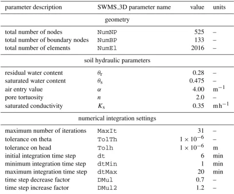
Table 1.Overview of the most relevant parameters in the SWMS 3D model.
parameter description SWMS 3D parameter name value units
geometry
total number of nodes NumNP 525 –
total number of boundary nodes NumBP 133 –
total number of elements NumEl 2016 –
soil hydraulic parameters
residual water content θr 0.28 –
saturated water content θs 0.475 –
air entry value α 4.00 m−1
pore tortuosity n 2.0 –
saturated conductivity Ks 0.35 m h−1
numerical integration settings
maximum number of iterations MaxIt 31 –
tolerance on theta TolTh 1×10⁻⁶ –
tolerance on head Tolh 1×10⁻⁶ m
initial integration time step dt 6 min
minimum integration time step dtMin 1 min
maximum integration time step dtMax 20 min
time step decrease factor DMul 0.7 –
time step increase factor DMul2 1.2 –
With the settings described above, we ran the reference model in order to generate artificial measurements fort=97 throught=216 h at hourly intervals. During the simulation, approximately 26.3 m3 of precipitation was applied. After the simulation ended, a total volume of about 15.7 m3 had been extracted vertically from the soil domain according to Eq. (5), while a total of about 12.1 m3was removed from the domain as seepage from the seepage face. At the end of the simulation period att=216 h, 186.5 m3of water was present in the soil, slightly less than the 188.0 m3of water that had been present att=96 h. Figure 3 shows how pressure head developed at the soil–bedrock interface for all nodes during the simulation period. Transient saturation occurred in about 60 % of the nodes, but dissipated relatively quickly for most nodes once precipitation stopped.
Upon completion of the run, we saved 3 variables: (1) the total volume of soil water that had been extracted according to Eq. (5); (2) the time series of discharge from the seepage face at the bottom of the hillslope; and (3) the space–time distributed pattern of pressure head at the soil–bedrock inter-face. That is, the first two variables describe integrated hy-drologic responses, whereas the third is spatially distributed. In parts 2 and 3 of this study (see Sects. 2.2 and 2.3, respec-tively), these 3 variables were then used as error-free artificial measurements with which to calibrate the simplified model; in part 4 (see Sect. 2.4), the SODA calibration from part 3 is repeated, but this time using only a subset of the artificial measurements, which were moreover perturbed in order to mimic the effect of measurement noise.
2.1.1 Simplified model and calibrated parameters
The simplified model differs only slightly from the reference model, in that it assumes that the sink is spatially homoge-neous. Equation (5) thus simplifies to
B=
(
0 h <0
rsink·h h≥0
. (6)
For field studies, it is common to make this assump-tion, even in cases where soft data suggest the presence of preferential-flow features such as cracks in the bedrock. Even though its validity may often be questionable, the modeler’s hand is forced by the lack of direct observations.
We calibrated 2 parameters: Ks, the saturated hydraulic conductivity (Eq. 3), and rsink, which controls the rate at which water is lost from the soil domain as it infiltrates the bedrock (Eq. 6).
2.2 SCEM-UA (idealized data set)
The Shuffled Complex Evolution Metropolis (SCEM-UA) algorithm has been discussed in detail elsewhere (e.g. Vrugt et al., 2003b); only a summary is presented here.
Fig. 3.Artificial measurements: simulated traces of pressure head in space and time. For each node at the soil–bedrock interface, the figure
contains a subplot showing a time series of the pressure head (magenta line) fort=97–216 h. Horizontal dashed lines represent zero pressure
head. Each subplot’s axes have been clipped vertically to [−0.5, 0.25] in order to better show the pressure head dynamics during relatively wet conditions. To further ease interpretation, each subplot was assigned a background color depending on how long saturated conditions lasted at a given location. The locations of sink hotspots are indicated with asterisks.
et al., 1992); but where SCE uses a multidimensional sim-plex to generate offspring, SCEM-UA uses Markov chains combined with a Metropolis-simulated annealing scheme (Metropolis et al., 1953; Kuczera and Parent, 1998).
Following the classical approach to inverse modeling, SCEM-UA assumes that the hydrological model structure
f (·)is a perfect description of the processes as they occur in reality, and that data errors are negligible. The model output vectorY is calculated using the model forcingsU by prop-agating the model initial stateX0using the model structure
f (·)and the model parametersθ:
Y=f (X0, U, θ ). (7)
The model output is compared with observationsZ, and the goodness-of-fit is expressed in an objective functiong(·):
OF=g(Y, Z), (8)
where OF represents the objective score. Points in the param-eter space thus become associated with an objective score. Note that the single-objective approach described here can be extended to include multiple objectives using the concept of Pareto optimality (Yapo et al., 1998; Gupta et al., 1998; Vrugt et al., 2003a).
1. Initialize a population of points in the parameter space, divide them over multiple complexes as per Duan et al. (1992);
2. When convergence has not been achieved, do
a. sample new points from the feasible parameter space;
b. determine the objective score OF for each point, by i. running the model
ii. running the objective function(s)
c. accept or reject each new point according to the Metropolis rule;
d. shuffle complexes;
e. calculate Gelman–Rubin convergence statistic (Gelman and Rubin, 1992).
SCEM-UA reliably finds the part of the parameter space that yields the best possible objective scores. It has been used suc-cessfully to identify model parameters in a variety of disci-plines including hydrology, soil chemistry, and ecology (e.g. Vrugt et al., 2003b, 2007; Nierop et al., 2002).
2.2.1 Objective functions
We use the following 3 functions to evaluate the performance of individual parameter combinations:
OF1= |ǫobs−ǫsim|, (9)
in whichǫobs andǫsim are the total observed and total sim-ulated vertical water loss, respectively. ǫ is calculated as
ǫ=Vinit+Vin−Vq−Vend, in whichVinitis the total volume of water that is present in the soil att=96 h,Vin is the to-tal volume of infiltration,Vqis the total volume of discharge
that is removed from the soil as seepage, andVendis the total volume of water that is present in the soil att=216 h;
OF2= v u u t 1
nt nt X
t=1
(qobs,t−qsim,t)2, (10)
in whichntis the number of time steps, andqobs,tandqsim,t
are the observed and simulated hillslope-scale discharge for thetth time step, respectively; and
OF3= v u u t 1
ni ni X
i=1
(hobs,i−hsim,i)2, (11)
in whichniis the product of the number of rows and columns
in the grid times the number of time steps, andhobs,i and
hsim,i are the observed and simulated pressure head at the
soil–bedrock interface for theith combination of row, col-umn and time step, respectively.
The rationale behind this combination of objective func-tions is as follows. The simplified model simulates redistri-bution of the available water, i.e. initial storage and infiltra-tion. The redistribution is subject to losses due to bedrock in-filtration (vertically) and seepage (laterally). Successful cal-ibration of the model requires that the volume of water that leaves the domain is accurate, which is achieved by minimiz-ing the first two objectives (Eqs. 9 and 10). However, the first two objectives are not capable of extracting any spatial in-formation. Using just the first two objectives could therefore lead to a proliferation of equally realistic solutions of pres-sure head patterns internal to the hillslope. To avoid that, the third objective (Eq. 11) attempts to use the spatial informa-tion in the pressure head data series, such that the soluinforma-tions that were equally realistic based on just the first two objec-tives can now be differentiated.
2.3 SODA (idealized data set)
The Simultaneous parameter Optimization and Data Assim-ilation (SODA Vrugt et al., 2005) algorithm may be viewed as an extension of SCEM-UA. It combines SCEM-UA’s pa-rameter estimation procedure with an ensemble Kalman fil-ter (EnKF; Evensen, 1994, 2003) such that uncertainty in the model states can be accommodated. SODA’s general struc-ture is therefore similar to the SCEM-UA strucstruc-ture outlined earlier, except that Step 2.b is different. Instead of running the model for all time steps at once, the EnKF generates an en-semble of model predictions, each of which having slightly different states. Each ensemble member is then propagated time step by time step, using the parameter combination sug-gested by the parameter estimation part of SODA. Step 2.b thus becomes
2.b. Determine the objective score OF for each point, by i. generating an ensemble of model states based on
the last a posteriori state (or the initial state); ii. propagating each ensemble member one time step,
using the model structure, the model forcings, and the parameter combination. This results in an a pri-ori state estimate for each ensemble member. Use the same parameter combination for all ensemble members and time steps;
iii. determining the magnitude and direction of the state updates by calculating the weighted average of the a priori state estimates and the observations (the weights are related to the degree of uncertainty in each component);
iv. adding the state updates to the a priori state esti-mates to get the a posteriori state estiesti-mates. v. returning to (i) if the current time is less than the
simulation end time; and
−3 −2.5 −2 −1.5 −1 −0.5
log
10
(rsink
)
100 200 300 400 500 600
−2 −1.5 −1 −0.5 0
model evaluation number
log
10
(Ks
)
Fig. 4.SCEM-UA (idealized data set): evolution of the parameters. Dashed lines represent value ofrsink(low)andrsink(high)(upper plot) and
Ks(lower plot). Markov chains are color-coded; open symbols are samples that have been rejected by the Metropolis scheme, while solid
colors have been accepted. Note that the vertical axes are logarithmic.
The major advantage of this approach is that, when errors are introduced on the model states (either as a result of errors in the model initial state, errors in the model forcings, or by the use of an imperfect model structure), their propagation through time is limited by the EnKF’s intermediate updating.
2.3.1 Objective functions
For water balance and discharge, we let SODA use the same objective functions and measurements that were used for SCEM-UA (Eqs. 9 and 10). The pressure head information, however, is used in a different way: rather than aggregating all errors using the objective function defined by Eq. (11), the pressure head measurements are used to update the a pri-ori model prediction in the EnKF. This is necessary in order to retain the timing and localization information pertaining to errors that may occur, and is therefore crucial for model improvement.
2.4 SODA (reduced and perturbed data set)
In part 4 of this study, we expand on the SODA results from part 3 by investigating whether SODA’s diagnostic capabil-ities are negatively affected when there are fewer measure-ments, and when those measurements are moreover subject to measurement noise. For this, we removed approximately half of the pressure head observation locations from the data set according to a random elimination pattern. Among the eliminated locations were two important sink hotspot loca-tions (X09Y15 and X00Y18). We then mimicked the effect of measurement noise by perturbing the remaining measure-ments. For the pressure head observations, we used zero-mean, homoscedastic Gaussian noise of standard deviation 0.005 m. The discharge measurements were perturbed using
a zero-mean, heteroscedastic Gaussian noise, with standard deviation equal to 10% of the true (unperturbed) discharge.
For water balance and discharge, we let SODA use the same objective functions that were used in part 3 (Eqs. 9 and 10). The pressure head information is applied in the same fashion as in part 3, although there are now fewer locations where measurements are available and the values that remain are now subject to measurement noise.
3 Results and discussion
3.1 SCEM-UA (idealized data set)
Figure 4 shows the evolution of the parameter distribution during the SCEM-UA calibration. Once the distribution be-comes stable after about 500 model evaluations, Ks is ac-curately and precisely identified, but thersinkparameter has settled on a range of values that represents neitherrsink(low)
norrsink(high). Because of the simplified model’s structural
deficiency, any value forrsink leads to errors somewhere in the hillslope. Forrsinkvalues close torsink(low), large errors
would be introduced at the locations of the hotspots – specif-ically, they would be too wet. The excess water at these lo-cations would subsequently lead to a plume of overestimated pressure heads downslope from each hotspot. However, the extent of the plumes is smaller forrsinkvalues that are some-what higher thanrsink(low). This is due to the combination of
Fig. 5.SCEM-UA (idealized data set): model-observation pressure head residuals in space and time, as associated with the Pareto-optimal
parameter combination log10(rsink)≈ −1.30; log10(Ks)≈ −0.47. For each node at the soil–bedrock interface, the figure contains a subplot
showing a time series of model-observation residuals (black line) fort=97–216 h. Horizontal dashed lines represent zero residual. To ease
interpretation of the residual pattern, each subplot was assigned a background color depending on the cumulative positive and cumulative negative residual: magenta colors represent under-estimation of artificial measurements (simulated value is too dry), while cyan means over-estimation (too wet). Note the spatial coherence and error propagation. The locations of sink hotspots as used in the reference model (but not the simplified model) are indicated with asterisks.
close to −2.0, even though the latter value is in fact the correct one for 93 out of 98 nodes. The side effect of these compensatory parameter values is that it becomes more difficult to determine the origin of the model struc-ture error. For example, Fig. 5 shows the difference between the simulated pressure head dynamics (generated using the Pareto-optimal parameter values log10(rsink)≈ −1.30 and log10(Ks)≈ −0.47) and the artificial measurements. The er-roneous parameterization leads to systematic deviations in pressure head for much of the hillslope, despite the fact that the simplified model differs only slightly from the reference model.
−3 −2.5 −2 −1.5 −1 −0.5
log
10
(rsink
)
100 200 300 400 500 600 700
−2 −1.5 −1 −0.5 0
model evaluation number
log
10
(Ks
)
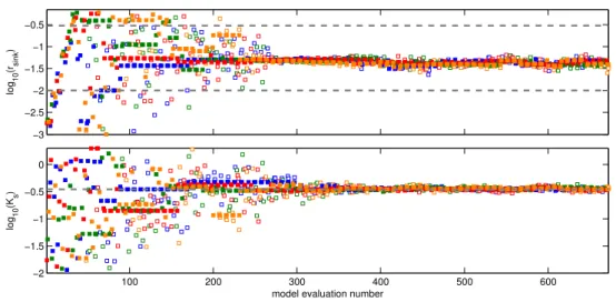
Fig. 6.SODA (idealized data set): evolution of the parameters. Dashed lines represent value ofrsink(low)andrsink(high)(upper plot) andKs
(lower plot). Markov chains are color-coded; open symbols are samples that have been rejected by the Metropolis scheme, while solid colors have been accepted. Note that the vertical axes are logarithmic.
3.2 SODA (idealized data set)
Figure 6 shows the evolution of the parameters during the SODA calibration. The figure shows that, after about 600 model evaluations, SODA draws exclusively from the narrow range around log10(Ks)≈ −0.45 and log10(rsink)≈ log10(rsink(low))= −2. The simplified model appliesrsink to all sink nodes at the soil–bedrock interface, leading to an overestimation of pressure heads at the hotspots. However, when this happens, the EnKF recognizes that the simulation is systematically deviating from the artificial measurements, and it updates the model states accordingly. Updating the model states (i.e. pressure head) downward equates to an ex-traction of water from the soil. However, since the updating is not part of the model structure itself but rather an effect of the state updating by SODA, we refer to it as an implicit sink term. Pressure head in the hillslope is thus affected by two flows that are part of the model (i.e. net lateral subsurface flow and the sink term of Eq. 6), as well as by the implicit sink that is external to the model. The implicit sink repre-sents any vertical losses that occur in excess of what Eq. (6) accounts for. Without the implicit sink, the lower part of the hillslope would be much too wet, which would in turn lead to biased optimal parameters.
From a model evaluation perspective, the state updates are interesting because they essentially form a record of how model structural error affects the model states. Moreover, the information contained within the record is specific to both a location and a time, making it possible to relate the magnitude and direction of state updates to physically rele-vant processes. Figure 7 shows the state updating that was performed when SODA evaluated the simplified model us-ing log10(rsink)≈ −1.97 and log10(Ks)≈ −0.46. Two types of responses can be distinguished in the figure: on the one
hand, most of the states do not need any updating. For those nodes, the simplified model provides an appropriate repre-sentation of the measurements, at least when the model is run with parameter values from the optimal range. On the other hand, there are other nodes that need substantial updat-ing (e.g. X00Y18, X06Y30, X09Y15, and X18Y09). These nodes coincide with hotspots. The structural difference be-tween the simplified model and the reference model leads to consistently deviating a priori estimates of pressure head in these areas, which are subsequently corrected by SODA. Further down, we explain why state updating is not limited to just the hotspots, but also occurs at nodes that are located close to hotspots.
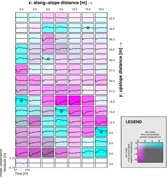
Fig. 7.SODA (idealized data set): pressure head state updates in space and time, as associated with the Pareto-optimal parameter combination
log10(rsink)≈ −1.97; log10(Ks)≈ −0.46. For each node at the soil–bedrock interface, the figure contains a subplot showing a time series
of state updates (black line) fort=97–216 h. Horizontal dashed lines represent zero updates (no adjustment). To ease interpretation of the
updating pattern, each subplot was assigned a background color that visually shows the magnitude of cumulative negative updating. Greener backgrounds mean stronger over-estimation (i.e. the model’s a priori value is too wet with respect to the artificial measurements). This figure uses a color scheme that is different from that of Fig. 5 to emphasize the difference in interpretation between model-observation residuals on the one hand and state updates on the other. The locations of sink hotspots as used in the reference model (but not the simplified model) are indicated with asterisks.
3.2.1 Limitations with respect to measurement interval
In this part, we are using an idealized data set without any measurement noise. As a result, the EnKF places much more confidence on the measurements than it does on the a pri-ori estimate of the model state: the a posteripri-ori model state is effectively determined by “resetting” the a priori model state to the value of the measurement. When the confidence balance is strongly in favor of the measurements, any errors that may have been introduced since the last measurement time are canceled almost completely after the states are up-dated at the time of the next measurement. However, if a lot
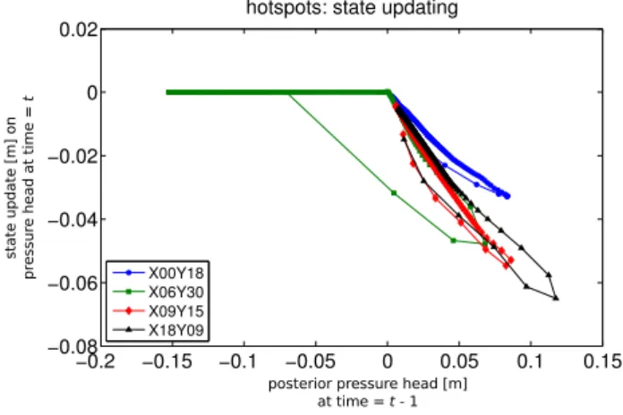
Fig. 8.SODA (idealized data set): state updating as a function of state value for 4 hotspot nodes. The data for this figure originate
from SODA’s evaluation of log10(rsink)≈ −1.97 and log10(Ks)≈
−0.46.
are taken at larger intervals, it is important that the measure-ment frequency is balanced with the timescale of the mod-eled process. Similarly, when individual measurements are associated with realistic measurement noise (as opposed to being error-free), the EnKF will not place as much confi-dence on the measurements. Consequentially, errors are not corrected as quickly, and the state updating pattern will be more difficult to interpret. This problem can be alleviated by measuring at smaller intervals, or by installing a more pre-cise measurement device. When setting up future field exper-iments, it may thus be worthwhile to increase the measuring frequency, even at the cost of the experiment’s duration.
3.2.2 Limitations with respect to information content
Besides balancing the measurement interval with the timescale of the process of interest, it also remains important that the measurements contain all relevant behavioral modes. This is because information content is more important than sheer data volume (e.g. Sorooshian et al., 1983; Gupta and Sorooshian, 1985); even powerful methods of analysis can-not extract information that is can-not present. For example, the reference model includes 5 hotspots, but only 4 of these can be identified from the SODA analysis. The reason for this is that the difference between the reference model and the sim-plified model only becomes apparent when saturated condi-tions occur at the location of one of the hotspots. If saturated conditions do not occur, the simplified model’s behavior can-not be distinguished from the reference model’s behavior: the sink termBis equal to zero for both models (compare Eqs. 5 and 6). Since saturated conditions did indeed not occur at X15Y39 (see Fig. 3), node X15Y39 cannot be identified as a hotspot from these measurements, regardless of the method used.
3.3 SODA (reduced and perturbed data set)
Figure 9 shows the evolution of the parameters during cal-ibration with SODA using the reduced and perturbed data set. ParameterKsis identified with similar accuracy and pre-cision as for the idealized data set, while parameterrsinkis slightly more uncertain and a very small bias has been in-troduced. The space–time pattern of state updating associ-ated with one of the Pareto-optimal parameter combinations is visualized in Fig. 10. In terms of magnitude, timing, and location, it is quite similar to the state updating associated with the idealized data set (Fig. 7). There are, however, some differences as well.
First there is the general appearance of state updating, which is much noisier here than for the idealized data set. This is because every state update is now partly a correction for the measurement noise that was introduced at the previ-ous time step. Because the magnitude of measurement noise is only small in comparison to the model uncertainty, and be-cause the measurement noise is not systematic, the noise does not negatively affect the state updating pattern as a whole.
−3 −2.5 −2 −1.5 −1 −0.5
log
10
(rsink
)
500 1000 1500 2000
−2 −1.5 −1 −0.5 0
model evaluation number
log
10
(K
s
)
Fig. 9.SODA (reduced and perturbed data set): evolution of the parameters. Dashed lines represent value ofrsink(low)andrsink(high)(upper
plot) andKs(lower plot). Markov chains are color-coded; open symbols are samples that have been rejected by the Metropolis scheme, while
solid colors have been accepted. Note that the vertical axes are logarithmic.
In summary, the analysis of SODA’s state updating helps to identify model deficiencies and provides us with the infor-mation necessary to improve our understanding of hydrolog-ical processes in an iterative cycle of modeling, experimental design, data collection, and analysis.
4 Conclusions
As models get more complex, there is a growing need for better tools with which to evaluate them (e.g. Beck, 1987; Gupta et al., 1998; Kirchner, 2006). It has been argued in the literature that model evaluation should not be limited to ranking model runs (differentiating between the good and the bad representations of the real world), but should also pro-vide some guidance on how to improve a given model struc-ture (Beck, 1987; Lin and Beck, 2007; Gupta et al., 2008). In this study, we purposely used a deficient model structure, which we calibrated both by a parameter estimation approach (SCEM-UA) and by a combined parameter and state estima-tion approach (SODA). We then assessed how suitable each method was for providing aforementioned guidance.
Four main conclusions that can be drawn from this work are
1. State adjustment patterns generated by SODA are help-ful in evaluating when and where model structural er-rors occur.
2. Relations can be constructed between SODA’s state ad-justments and the model states themselves. Such rela-tions can readily be adopted in an improved version of the model. Perhaps most importantly, they stimulate the discussion between modeler and experimentalist about what process could explain them, while at the same
time guiding the discussion by setting constraints on the functional form of the relation.
3. For a reduced and perturbed data set, SODA proved useful in identifying the location of some hotspots, as well as the functional relation driving the model struc-ture error. Due to gaps in the spatial distribution of mea-surements, some other hotspots could not be identified, although the space–time pattern of state updating did show the general area where model structure errors were introduced.
4. SCEM-UA cannot provide information that is as in-formative as that provided by SODA. Parameter es-timation methods such as SCEM-UA lack a strategy with which the propagation of errors is reduced. Due to compensation effects, tuning the parameters of a struc-turally deficient model may therefore result in optimal parameter values without any physical relevance. This inhibits a straightforward interpretation of the model-observation residuals with regard to model improve-ment.
By using artificially generated measurements, we were able to focus strictly on the usefulness of the algorithms, while avoiding any issues relating to the quality of measure-ments.
5 Next steps
Fig. 10.SODA (reduced and perturbed data set): pressure head state updates in space and time. These state updates are associated with
the Pareto-optimal parameter combination log10(rsink)≈ −2.13; log10(Ks)≈ −0.46. Where pressure head observations were available, the
figure contains a subplot showing a time series of state updates at the soil–bedrock interface (black line) fort=97–216 h; the other nodes
have been grayed out. Horizontal dashed lines represent zero updates (no adjustment). To ease interpretation of the updating pattern, each subplot was assigned a background color that visually shows the magnitude of cumulative negative updating. Greener backgrounds mean stronger over-estimation (i.e. the simplified model’s a priori value is too wet with respect to the artificial measurements). This figure uses a color scheme that is different from that of Fig. 5 to emphasize the difference in interpretation between model-observation residuals on the one hand and state updates on the other. The locations of sink hotspots as used in the reference model (but not the simplified model) are indicated with asterisks.
Fig. 11.SODA (reduced and perturbed data set): state updating as a function of state value for selected nodes. The data for this figure
are facing when we study hydrological dynamics of catch-ments. While this study has focused on improved analysis of simulation-measurement discrepancies, various other aspects also play a role in successfully learning from experimenta-tion. For these aspects, continued experimentation with arti-ficial measurements can be of great value, for instance when investigating the effect of spatially distributed soil proper-ties or the effect of uncertainproper-ties in the model forcings. Po-tentially, there are many such effects influencing the model state, and we do not claim that the proposed analysis is the way to identify all of them. Nonetheless, SODA’s state up-dating will certainly help to provide the information neces-sary to improve our understanding of hydrological processes in an iterative cycle of modeling, experimental design, data collection and analysis.
Supplementary material related to this article is
available online at: http://www.hydrol-earth-syst-sci.net/ 17/3455/2013/hess-17-3455-2013-supplement.zip.
Acknowledgements. The authors would like to thank Erwin Zehe
for serving as editor on this paper. Thanks also to two anonymous reviewers, whose constructive comments improved the manuscript. We further wish to express our gratitude to J. A. Vrugt, for kindly providing the algorithms, and for his many useful comments on an earlier version of this manuscript. This work is part of the program of BiG Grid, the Dutch e-Science Grid, which is financially supported by the Nederlandse Organisatie voor Wetenschappelijk Onderzoek (Netherlands Organisation for Scientific Research, NWO). Further funding was provided by the Netherlands eScience Center (http://www.esciencecenter.nl) which is supported by SURF and NWO. N. S. Anders, M. U. Kemp, J. D. McLaren, L. E. Veen, I. Soenario and W. Vansteelant are thanked for their constructive criticism during the writing of this manuscript.
Edited by: E. Zehe
References
Ajami, N. K., Duan, Q., and Sorooshian, S.: An integrated hy-drologic Bayesian multimodel combination framework: con-fronting input, parameter, and model structural uncertainty in hydrologic prediction, Water Resour. Res., 43, W01403, doi:10.1029/2005WR004745, 2007.
Bastidas, L. A., Hogue, T. S., Sorooshian, S., Gupta, H. V., and Shuttleworth, W. J.: Parameter sensitivity analysis for different complexity land surface models using multicriteria methods, J. Geophys. Res., 111, D20101, doi:10.1029/2005JD006377, 2006. Beck, M. B.: Water quality modeling: a review of the anal-ysis of uncertainty, Water Resour. Res., 23, 1393–1442, doi:10.1029/WR023i008p01393, 1987.
Beven, K. and Binley, A.: The future of distributed models: model calibration and uncertainty prediction, Hydrol. Process., 6, 279– 298, 1992.
Bl¨oschl, G. and Sivapalan, M.: Scale issues in hydrological mod-elling – a review, Hydrol. Process., 9, 251–290, 1995.
Box, G. E. P. and Tiao, G. C.: Bayesian Inference in Statistical Anal-ysis, Addison-Wesley-Longman, Reading, Massachusetts, 1973. Boyle, D. P., Gupta, H. V., and Sorooshian, S.: Toward improved calibration of hydrologic models: combining the strengths of manual and automatic methods, Water Resour. Res., 36, 3663– 3674, 2000.
Boyle, D. P., Gupta, H. V., Sorooshian, S., Koren, V., Zhang, Z., and Smith, M.: Toward improved streamflow forecasts: value of semidistributed modeling, Water Resour. Res., 37, 2749–2759, doi:10.1029/2000WR000207, 2001.
Clark, M. P. and Vrugt, J. A.: Unraveling uncertainties in hydrologic model calibration: addressing the problem of compensatory parameters, Geophys. Res. Lett., 33, L06406, doi:10.1029/2005GL025604, 2006.
Clark, M. P., Slater, A. G., Rupp, D. E., Woods, R. A., Vrugt, J. A., Gupta, H. V., Wagener, T., and Hay, L. E.: Framework for Under-standing Structural Errors (FUSE): a modular framework to di-agnose differences between hydrological models, Water Resour. Res., 44, W00B02, doi:10.1029/2007WR006735, 2008. Doherty, J. and Welter, D.: A short exploration of structural noise,
Water Resour. Res., 46, W05525, doi:10.1029/2009WR008377, 2010.
Duan, Q., Gupta, V. K., and Sorooshian, S.: Effective and efficient global optimization for conceptual rainfall-runoff models, Water Resour. Res., 28, 1015–1031, 1992.
Dunn, S. M.: Imposing constraints on parameter values of a concep-tual hydrological model using baseflow response, Hydrol. Earth Syst. Sci., 3, 271–284, doi:10.5194/hess-3-271-1999, 1999.
Efstratiadis, A. and Koutsoyiannis, D.: One decade of
multi-objective calibration approaches in
hydrologi-cal modelling: a review, Hydrolog. Sci. J., 55, 58–78, doi:10.1080/02626660903526292, 2010.
Eigbe, U., Beck, M. B., Wheater, H. S., and Hirano, F.: Kalman filtering in groundwater flow modelling: prob-lems and prospects, Stoch. Hydrol. Hydraul., 12, 15–32, 1doi:0.1007/s004770050007, 1998.
Evensen, G.: Sequential data assimilation with a nonlinear quasi-geostrophic model using Monte Carlo methods to forecast error statistics, J. Geophys. Res., 99, 10143–10162, 1994.
Evensen, G.: The Ensemble Kalman Filter: theoretical formula-tion and practical implementaformula-tion, Ocean Dynam., 53, 343–367, doi:10.1007/s10236-003-0036-9, 2003.
Franks, S. W., Gineste, P., Beven, K. J., and Merot, P.: On constrain-ing the predictions of a distributed model: the incorporation of fuzzy estimates of saturated areas into the calibration process, Water Resour. Res., 34, 787–797, doi:10.1029/97WR03041, 1998.
Gelman, A. and Rubin, D. B.: Inference from Iterative Simula-tion Using Multiple Sequences, available at: http://www.jstor. org/stable/pdfplus/2246093.pdf, Stat. Sci., 7, 457–472, 1992. Georgakakos, K. P., Seo, D., Gupta, H., Schaake, J., and
Butts, M. B.: Towards the characterization of streamflow simula-tion uncertainty through multimodel ensembles, J. Hydrol., 298, 222–241, doi:10.1016/j.jhydrol.2004.03.037, 2004.
Gupta, H. V., Sorooshian, S., and Yapo, P. O.: Toward improved cal-ibration of hydrologic models: multiple and noncommensurable measures of information, Water Resour. Res., 34, 751–763, 1998. Gupta, H. V., Wagener, T., and Liu, Y.: Reconciling theory with observations: elements of a diagnostic approach to model eval-uation, Hydrol. Process., 22, 3802–3813, doi:10.1002/hyp.6989, 2008.
Gupta, V. K. and Sorooshian, S.: The relationship between data and the precision of parameter estimates of hydrologic models, J. Hy-drol., 81, 57–77, 1985.
Hoeting, J. A., Madigan, D., Raftery, A. E., and Volinsky, C. T.: Bayesian model averaging: a tutorial, Stat. Sci., 14, 382–401, 1999.
Hopp, L. and McDonnell, J. J.: Connectivity at the hillslope scale: Identifying interactions between storm size, bedrock permeabil-ity, slope angle and soil depth, J. Hydrol., 376, 378–391, 2009. Jazwinski, A. H.: Stochastic Processes and Filtering Theory,
Aca-demic Press, New York, 1970.
Kalman, R. E.: A new approach to linear filtering and prediction
problems, available at: http://www.cs.unc.edu/∼welch/kalman/
media/pdf/Kalman1960.pdf, T. ASME J. Basic Eng., 82, 35–45, 1960.
Kavetski, D., Kuczera, G., and Franks, S. W.: Bayesian analysis of input uncertainty in hydrological modeling: 1. Theory, Water Resour. Res., 42, W03407, doi:10.1029/2005WR004368, 2006a. Kavetski, D., Kuczera, G., and Franks, S. W.: Bayesian analysis of input uncertainty in hydrological modeling: 2. Application, Water Resour. Res., 42, W03408, doi:10.1029/2005WR004376, 2006b.
Kirchner, J. W.: Getting the right answers for the right rea-sons: linking measurements, analyses, and models to advance the science of hydrology, Water Resour. Res., 42, W03S04, doi:10.1029/2005WR004362, 2006.
Kleme˘s, V.: Operational testing of hydrological simulation models, Hydrolog. Sci. J., 31, 13–24, 1986.
Kuczera, G. and Mroczkowski, M.: Assessment of hydrologic pa-rameter uncertainty and the worth of multiresponse data, Water Resour. Res., 34, 1481–1489, doi:10.1029/98WR00496, 1998. Kuczera, G. and Parent, E.: Monte Carlo assessment of parameter
uncertainty in conceptual catchment models: the Metropolis al-gorithm, J. Hydrol., 211, 69–85, 1998.
Lin, Z. and Beck, M. B.: On the identification of model structure in hydrological and environmental systems, Water Resour. Res., 43, W02402, doi:10.1029/2005WR004796, 2007.
Metropolis, N., Rosenbluth, A. W., Rosenbluth, M. N., Teller, A. H., and Teller, E.: Equations of state calculations by fast computing machines, J. Chem. Phys., 21, 1087–1091, 1953.
Mroczkowski, M., Raper, G. P., and Kuczera, G.: The quest for more powerful validation of conceptual catchment models, Water Re-sour. Res., 33, 2325–2335, 1997.
Neuman, S. P.: Maximum likelihood Bayesian averaging of uncer-tain model predictions, Stoch. Env. Res. Risk A., 17, 291–305, doi:10.1007/s00477-003-0151-7, 2003.
Nierop, K. G. J., Jansen, B., Vrugt, J. A., and Verstraten, J. M.: Cop-per complexation by dissolved organic matter and uncertainty assessment of their stability constants, Chemosphere, 49, 1191– 1200, 2002.
Popper, K.: The Logic of Scientific Discovery, Routledge, first published as Logik der Forschung, 1935 by Verlag von Julius
Springer, Vienna, Austria, 2009.
Raftery, A. E., Balabdaoui, F., Gneiting, T., and Polakowski, M.: Using Bayesian Model averaging to calibrate forecast ensembles, Tech. rep., Department of Statistics, University of Washington, Seattle, Washington, 2003.
Raftery, A. E., Gneiting, T., Balabdaoui, F., and Polakowski, M.: Using Bayesian Model averaging to calibrate forecast ensembles, Mon. Weather Rev., 133, 1155–1174, 2005.
Reusser, D. E. and Zehe, E.: Inferring model structural deficits by analyzing temporal dynamics of model performance and parameter sensitivity, Water Resour. Res., 47, W07550, doi:10.1029/2010WR009946, 2011.
Richards, L. A.: Capillary conduction of liquids through porous mediums, Physics, 1, 318–333, 1931.
Schoups, G. and Vrugt, J. A.: A formal likelihood function for pa-rameter and predictive inference of hydrologic models with cor-related, heteroscedastic, and non-Gaussian errors, Water Resour. Res., 46, W10531, doi:10.1029/2009WR008933, 2010. Seibert, J.: Multi-criteria calibration of a conceptual runoff model
using a genetic algorithm, Hydrol. Earth Syst. Sci., 4, 215–224, doi:10.5194/hess-4-215-2000, 2000.
Sieber, A. and Uhlenbrook, S.: Sensitivity analyses of a distributed catchment model to verify the model structure, J. Hydrol., 310, 216–235, 2005.
˘Sim˚unek, J.: SWMS 3D – numerical model of three-dimensional flow and solute transport in a variably saturated porous medium, software, avaiable at: http://www.pc-progress.com/Downloads/ Programs UCR/SWMS 3D.zip (last access: 2 February 2013), 1994.
˘Sim˚unek, J., Huang, K., and van Genuchten, M. T.: The SWMS 3D Code for Simulating Water Flow and Solute Transport in Three-Dimensional Variably-Saturated Media, US Salinity Laboratory, Agricultural Research Service, Research Report No. 139, US De-partment of Agriculture, Riverside, California, 1995.
Sorooshian, S., Gupta, V. K., and Fulton, J. L.: Evaluation of max-imum likelihood parameter estimation techniques for conceptual rainfall-runoff models: influence of calibration data variability and length on model credibility, Water Resour. Res., 19, 251– 259, doi:10.1029/WR019i001p00251, 1983.
Spear, R. C. and Hornberger, G. M.: Eutrophication in peel in-let – II. Identification of critical uncertainties via generalized sensitivity analysis, Water Res., 14, 43–49, doi:10.1016/0043-1354(80)90040-8, 1980.
Tang, Y., Reed, P., and Wagener, T.: How effective and effi-cient are multiobjective evolutionary algorithms at hydrologic model calibration?, Hydrol. Earth Syst. Sci., 10, 289–307, doi:10.5194/hess-10-289-2006, 2006.
van Genuchten, M. T.: A closed-form equation for predicting the hydraulic conductivity of unsaturated soils, Soil Sci. Soc. Am. J., 44, 892–898, 1980.
von Bertalanffy, L.: The theory of open systems in physics and bi-ology, Science, 111, 23–29, 1950.
Vrugt, J. A., Gupta, H. V., Bastidas, L. A., Bouten, W., and Sorooshian, S.: Effective and efficient algorithm for multi-objective optimization of hydrologic models, Water Resour. Res., 39, 1214, doi:10.1029/2002WR001746, 2003a.
Wa-ter Resour. Res., 39, 1201, doi:10.1029/2002WR001642, 2003b. Vrugt, J. A., Diks, C. G. H., Gupta, H. V., Bouten, W., and Verstraten, J. M.: Improved treatment of uncertainty in hydro-logic modeling: combining the strengths of global optimiza-tion and data assimilaoptimiza-tion, Water Resour. Res., 41, W01017, doi:10.1029/2004WR003059, 2005.
Vrugt, J. A., van Belle, J., and Bouten, W.: Pareto front anal-ysis of flight time and energy use in long-distance bird migration, J. Avian Biol., 38, 432–442, doi:10.1111/j.0908-8857.2007.03909.x, 2007.
Wagener, T., Boyle, D. P., Lees, M. J., Wheater, H. S., Gupta, H. V., and Sorooshian, S.: A framework for development and applica-tion of hydrological models, Hydrol. Earth Syst. Sci., 5, 13–26, doi:10.5194/hess-5-13-2001, 2001.
Wagener, T., McIntyre, N., Lees, M. J., Wheater, H. S., and Gupta, H. V.: Towards reduced uncertainty in conceptual rainfall-runoff modelling: dynamic identifiability analysis, Hydrol. Pro-cess., 17, 455–476, doi:10.1002/hyp.1135, 2003.
Western, A. W. and Bl¨oschl, G.: On the spatial scaling of soil mois-ture, J. Hydrol., 217, 203–224, 1999.
Yapo, P. O., Gupta, H. V., and Sorooshian, S.: Multi-objective global optimization for hydrological models, J. Hydrol., 204, 83–97, 1998.
Young, P.: A general theory of modeling for badly defined dy-namic systems, in: Modeling, Identification and Control in En-vironmental Systems – Proceedings of the IFIP Working Con-ference on Modeling and Simulation of Land, Air, and Water Resources Systems, edited by: Vansteenkiste, G. C., 103–135, North-Holland Pub. Co., Amsterdam, 1978.
Young, P.: Uncertainty and forecasting of water quality, in: The Validity and Credibility of Models for Badly Defined Systems, Springer Verlag, 69–98, 1983.