MATHEMATICAL APPROACH FOR DRILLING

(1)

International Journal of Automotive and Mechanical Engineering (IJAME)

ISSN: 2229-8649 (Print); ISSN: 2180-1606 (Online); Volume 3, pp. 318-340, January-June 2011 ©Universiti Malaysia Pahang

DOI: http://dx.doi.org/10.15282/ijame.3.2011.8.0027

318

MATHEMATICAL APPROACH FOR DRILLING

Hussien Mahmoud Al-Wedyan1 and Saad A Mutasher2

1

Department of Mechanical Engineering, Al Huson University College Al-Balqa’ Applied University

PO Box 50, Al Huson 21510, Jordan

2

School of Engineering, Computing and Sciences Swinburne University of Technology (Sarawak Campus) Jalan Simpang Tiga, 93350, Kuching, Sarawak, Malaysia

Email: [email protected]

ABSTRACT

The present paper is on the study of whirling dynamics of the tool workpiece system in a deep hole machining process. An innovative analytical model is proposed in order to carry out simulation studies on the whirling vibrations of the tool workpiece system in a deep hole boring process. At the interaction point of the boring bar-workpiece system there will be an additional displacement in addition to the torque transmitted. This displacement is of a dynamic origin and could be simulated as a wedge introduced between the cutting head-workpiece assemblies. An assumed mode method with the Lagrangian equations was used to derive the mathematical model of the system.

Keywords: Whirling vibration, mode shape, drilling process, mathematical model.

INTRODUCTION

The deep hole boring process is used to bore holes with usually high length to diameter ratios seeking better surface finish, good roundness and straightness. The process usually depends upon the following hole requirements: diameter of the bored hole, the depth of the bored hole, the characteristics of the hole surface, the dimensions, correctness, parallelism and straightness. Due to the fact that the boring bar-cutting head combination is slender, which is essential to produce holes with different diameter to length ratios, this kind of drilling is subject to disturbances such as chattering vibrations. Despite the abundance of studies done in this field, chatter vibrations are still not fully understood. Whirling motion is vibration in three dimensions, which affects the accuracy of the bored piece. It is well known now that the deep hole boring process is used extensively to drill expensive workpieces and hence process precision is of prime importance. To achieve the best process plan with the aim of minimizing the risk of the workpiece damage, a comprehensive investigation of the dynamics involved in the process, both analytically and experimentally, is highly important.

Over the last twenty years, there have been increased research efforts to investigate the chatter vibration. The regenerative vibration effect was investigated (Bayly et al., 2002). Their model was used to investigate cutting and rubbing forces in a chisel drilling edge in addition to tool vibration, which causes error in the hole size, or

(2)

Al-Wedyan and Mutasher / International Journal of Automotive and Mechanical Engineering 3(2011) 318-340

319

phenomena occur. Also, undesirable vibrations were expected due to the length of the BTA drill with low torsional and bending stiffness. A mechanism of torsional chatter was investigated experimentally (Bayly et al., 2001). The analysis was carried out in the frequency domain to find the chatter frequencies and boundaries of stability. The engagement and disengagement is highly non-linear during the drilling process and highly dynamic. A mathematical model was presented for a chisel drill with a zero helix angle to determine the displacement of the assumed rigid tool and rigid workpiece, but considering only the axial vibrations and ignoring the transverse motion (Batzer et al., 2001). They used a single degree of freedom model that was solved numerically to find the chip thickness and the time lag for the chip formation. Cutting tests were done and theoretically correlated the acoustic emission during cutting to the workpiece-tool geometry and the cutting conditions to verify the results (Keraita et al., 2001). They showed that the instability of cutting or chatter is due to a combination of structure, cutting conditions and tool geometry. Litak et al. (1997) theoretically investigated the chaotic harmful chatter vibrations which caused instabilities during the cutting process. The quasi-static model was used to study the roundness error in reaming due to regenerative vibration (Bayly et al., 2001). It was shown that a tool with N teeth caused a hole with N+1 or N-1 “lobes” which are related directly to the forward and backward whirl motion. Whirling vibrations were experimentally measured by Fujii et al. (1986a) in order to investigate how the whirling vibrations developed in the chisel drill. They used three different chisel drills with different web thickness. Fujii et al. (1986b) studied the interactions between the effect of the drill geometry and the drill flank, in starting whirling and developing it, and found also that the flank surface of the cutting edge is responsible for damping the vibration. Fujii et al. (1988) investigated the whirling vibrations in a workpiece having a pilot hole, and found that the whirling motion is a regenerative vibration caused by cutting forces and friction while drilling. The dynamics of the BTA deep hole boring process were statistically investigated experimentally by Weinert et al. (1999), who showed that disturbances like chatter and spiralling caused roundness and straightness error in the bored workpiece due to the high length to diameter ratio of the boring bar. Ema et al. (1988) carried out an experimental investigation on long drills with different lengths and special mass added to them. The results show that chatter is a self-induced vibration and the frequency of chatter is equal to the frequency of the natural bending frequency of the drill.

In spite of several studies done theoretically and experimentally to explore and understand the chatter phenomenon, it is not fully understood. From the previous review we can say that the regenerative effect of the chatter vibrations has not been taken into consideration in the cutting process, although some include the regenerative effect in their study. Some models assume a single degree of freedom or twodegrees of freedom in their models, which in some way simplifies the analysis. In general, no study has been done on the whirling vibrations in the deep hole boring process.

MATHEMATICAL MODELLING OF THE BORING BAR DYNAMICS

(3)

Mathematical approach for drilling

320

Figure 1. Boring Trepanning Association deep hole drilling machine

During the machining process, depending upon the degree of stability, the boring bar with the cutting tool attached to it can be considered to be subject to different end conditions. A mathematical model of the boring bar system is suggested on the basis of the following: first, the boring bar is considered as a continuous beam clamped at the driver end, with the stiffness at the end infinite. Second, an intermediate support is provided to the boring bar by the pressure head and proper type of stuffing box provided at the contact point, so that a simple support condition is assumed at the contact point.

Figure 2. Model of the boring bar assembly

The boring bar system will be considered as a multi-span beam, as shown in Figure 2, and the transverse vibrations of the multi-span beam are studied initially. When the boring bar undergoes a transverse vibration, the governing partial differential equation is given by:

 

Χ,t 0, j 1,2 t

w

Μ

t

Χ, Χ

w

ΕΙ ₂j

2

4 j 4

  

  



(4)

321 where

g

ΰ

Μ  , and EI is the bending rigidity of the material.

The solution of Eq. (1) is obtained by the separation of variables technique where we assume:

 

Χ,t ς

   

Χ Ρt

wj  j (2)

Substituting Eq. (2) into Eq. (1) results in Eq. (3)

 

Χ ί ς

 

Χ 0

ς j

4 '

'' '

j   , j1,2 (3)

and

 

t ω Ρ

 

t 0

P  2  (4)

where

g

ΕΙ ΰ

L

ω ί4 _ 2 4

The solutions of Eq. (3) for the two regions are

 

Χ cosίΧ coshίΧ C sinίΧ DsinhίΧ

ς1  1  1  1  1 (5)

 

Χ cosίΧ coshίΧ C sinίΧ D sinhίΧ

ς2  2  2  2  2 (6)

and the solution of Eq. (4) is of the form

 

t Fcos t Qsinωt

Ρ    (7)

The functions ς₁

 

Χ and ς₂

 

Χ have to satisfy the conditions that their respective fourth derivatives are equal to a constant multiplied by the functions as stated in Eq. (3). All the constants ₁,₁,C₁,D₁,₂,₂,C₂andD₂are evaluated using the following boundary conditions:

 

₂

 

₁

 

₁ ₂

 

₂ 1

2 2 1 1 2

1

L '

ς

L

ς'

0, 0 ' ' '

ς

0

ς'

L ' ' L ' ' 0

L

ς

L

ς

0, 0 ' '

ς

0

ς

  



 

 ₁ ₁ ₂ ₂

(8)

Substituting the boundary conditions into the equations will end up with 8 equations in terms of the 8 constants A_i,B_i,C_iandD_i,i1,2. The determinant of the coefficient matrix will give us the frequency equation. So for different values of L₁/ L₂, the frequency equation is expressed in Eq. (9):

 

   

       

 

   

 

   

0

4

4 4

4

4 4

2 2

1 1

2 2

1 1

2 2

1 1

2 2

1 1

2 2

1 1

2 2

 

 



 

 

L cos L cosh L sinh L cos

L sin L cosh L

sin L cosh L

sinh L cos

L sin L cos L cos L cosh L

cos L cosh L sin L cosh

L sin L cosh L cos L cosh L

sinh L cos

 

(9)

(5)

322

A comparison between the calculated natural frequency and the natural frequency calculated by Chandrashekhar (1984) shows an exact match, as in Table 1.

Table 1. The first five natural frequencies of the cutting tool-boring bar system

 n (rad/s) n (rad/s)-Chandrashekhar

3.912 453.77 453.76

7.043 1470.80 1470.47

10.173 3068.57 3068.02

13.302 5247.30 5246.50

16.432 8006.08 8005.91

MATHEMATICAL MODELLING OF THE BORING BAR-WORKPIECE DYNAMICS (MODEL–1)

The cutting tool-boring bar-workpiece system will be considered as a multi-span beam as shown in Figure 3 and assuming it is without a simple support at the boring bar for model-1.

Figure 3. Model of the cutting tool boring bar-workpiece system

The transverse vibration of the boring bar-workpiece in the Y-Z plane, which is the plane of symmetry, is formulated. It is described by two partial differential equations, the first one to represent the boring bar-cutting tool and the second to represent the workpiece as follows:

 

Χ,t 0, j 1 t

w

Μ

t

Χ, Χ

w

ΕΙ ₂j

2

4 j 4

  

  



1

1 (10)

 

₂

 

2

2 _  

  



j 0, t

Χ,

t w

Μ

t

Χ, Χ

w

ΕΙ ₂j

2

4 j 4

(6)

323

where ₁ Α₁

g

γ

Μ  ; ₂ Α₂

g

γ

Μ  ;









2

2 4

2 2 2 1

4 4 1

4 64

4

64 d di and A d di , dw and A dw

 



 _ _ _ _ _ _



 _ _

Solving these equations by the separation of variables technique, it is assumed that

 

Χ,t ς

   

Χ Ρ t

wj  j (12)

Substituting Eq. (12) in Eq. (10) and Eq. (11) results in

 

Χ ί ς

 

Χ 0

ς j

4 ''

''

j   , j1,2 (13)

 

t ω Ρ

 

t 0

P  2 

 ₍₁₄₎

where

g

ΕΙ ΰ

L

ω

ί4  2 4

;

2 1

1 2 2

2 1

    

  

  

  

 

  

   

 ( ) g

L L

n ;

2 1

) (

EI EI  

2

L

ί η

, L

ί

η1 1 2 

The solution for Eq. (13) is

 

Χ cosίΧ coshίΧ CsinίΧ DsinhίΧ

ς1  1  1  1  1 (boring bar) (15)

 

Χ cosίΧ coshίΧ C sinίΧ DsinhίΧ

ς2  2  2  2  2 (workpiece) (16)

and the solution of Eq. (14) is of the form

 

t Fcos t Qsinωt

Ρ    (17)

The functionsς₁

 

Χ , ς₂

 

Χ have to satisfy the conditions that their respective fourth derivatives are equal to a constant multiplied by the functions. All the constants ₁,₁,C₁,D₁,₂,₂,C₂ andD₂ are evaluated using the following boundary conditions:

 

L ,t W



L ,t



, W

, ,t 0 ' W 0,t ' W

0, 0,t W 0,t

W ₂

2 2 1

1

2 1

1

0



 

 





 





 

L ,t W '''



L ,t



, '

' ' W

, t , L ' ' W t , L ' ' W

, t , L ' W t , L ' W

2 2 1

1

2 2 1

1

2 2 1

1

 

 

(18)

(7)

324

Table 2. The first five natural frequencies of the cutting tool-boring bar system for model-1

 n (Hz)

1.56 11.49

2.81 37.282

4.09 78.984

5.37 136.15

6.6 205.675

Hence, the Mode shape functions are

 

_                                  1 1 1 1 1 1 L ax sinh L ax sin L ax cosh L ax cos

X *

 (19)

 

_                                        2 2 3 2 2 2 2 L bx sinh L bx sin L bx cosh L bx cos

X * *

 (20)

where aL₁, bL₂

   

 





 





 





 









   

  



  







  



  



 

   

 





  



  



  



 









   

 





 

b cosh



a b



sinh

  

b cos a b



sinh

  

b cos a b



sin b a cosh b sin b cosh a sin b cos a sinh b a sinh b a sin a sinh a sin b a sin b cosh b a sin b cosh b a sin b cos b a sinh b cos b sin a cosh b sinh a cos b sinh a sin b a cos b cosh b a cos b cosh b a cos b a sin b sinh b a sin b sin b cos a cosh b a cosh b a sinh b sin b a sinh b sin b cosh a cos a cosh a cos b a cosh b cos b a cosh b cos b sin a sinh                                                     2 2 2 2 2 2 2 2 2 2 2 2 2 2 2 2 1  (21)

 





  



  



 





 









 





 





  



  



   

 

  



  



 

b sinh



a b



cos

 

b sinh



a b



cosh

   

a sin b cos

 

a sinh

 

b cos b a sin b cosh b a sin b cosh b cosh a sin b cos a sinh b a cos b sinh b a cos b sinh b a cosh b sin b a cosh b sin b a sin b a sinh a sinh a sin b a cosh a sin b a cos a sinh b a sin a cosh b a sinh a cos b sinh b sin 2 2 2 2 2 2 2 2 2 2 2 2 2 2 2                                    

(8)

325

   

 





 





 





 









   

  



  







  



  



 

   

 





  



  



  



 









   

 





 

b cosh



a b



sinh

  

b cos a b



sinh

  

b cos a b



sin

b a cosh b sin b cosh a sin b cos a sinh b

a sinh

b a sin a sinh a

sin b

a sin b cosh b

a sin b cosh

b a sin b cos b a sinh b cos b sin a cosh b

sinh a cos

b sinh a sin b a cos b cosh b

a cos b cosh b

a cos

b a sin b sinh b

a sin b sin b cos a cosh b

a cosh

b a sinh b sin b a sinh b sin b cosh a cos a cosh

a cos b

a cosh b cos b a cosh b cos b sin a sinh

 

 

 

 

 

 

 

 

 

 

  

 

 

 

  

 

 

 

  

 



2 2

2

2 2

2

2 2

3

 (23)

Table 3.The first five natural frequencies of the cutting tool-boring bar-workpiece system.

Mode No. _r ₁ ₂ ₃ _n(rad/s)

1 2.025 -0.9677 -0.1466 0.8931 120.992

2 4.191 -0.9939 -0.0967 3.2701 520.573

3 6.282 -0.9998 0.0037 2.0247 1169.42

4 8.201 -1.0000 0.0005 -0.1207 1993.80

5 10.220 -1.0000 0.0001 -2.5607 3097.101

MATHEMATICAL MODELLING OF THE CUTTING TOOL-BORING BAR-WORKPIECE DYNAMICS (MODEL-2)

Model-2 will be assumed to have a simple support at the boring bar. During the machining process, the interaction point between the cutting tool head and the workpiece is shown in Figure 4. The moment, force, slope and deflection are assumed to be equal on the left and right hand side of the interaction point.

Figure 4. Model-2 of cutting tool-boring bar-workpiece system

(9)

326

 

Χ,t 0, j 1,2, t

w

Μ Χ,t Χ

w

ΕΙ ₂j

2

4 j 4

  

  



1

1 (24)

 

₂

 

34

2 Χ,t 0, j ,

t w

Μ Χ,t Χ

w

ΕΙ ₂j

2

4 j 4

  

  



(25)

where ₁ ₁

g

ΰ

Μ  ; ₂ ₂

g

ΰ

Μ  ;









2

2 4 2

2 2 1

4 4 1

4 64

4

64 d di ;A d di , dw ;A dw

 

 

 

 



 _ _

Solving these equations by the separation of variables technique is assumed that

 

Χ,t ς

   

Χ Ρ t

w_j  _j (26)

Substituting Eq. (26) into Eq. (24) and Eq. (25) results in

 

Χ ί ς

 

Χ 0

ς j

4 '

'' '

j   , j1,2,3 (27)

 

t ω Ρ

 

t 0

Ρ _ 2 _

, (28)

ΕΙ ΰ

L

ω

ί4  2 4

;

2 1

1 2 2

3 2 1

2 1 1

    

  

  

  

 

 

  

    

 ( ) g

L L L

*

n and

2 1

) (

EI EI  

3

L

ί η

, L

ί η

, L

ί

η1  1 1  2 2 



The solution for Eq. (27) is

 

ς1  1  1  1  1 (29)

 

ς2  2  2  2  2 (30)

 

ς3  3  3  3  3 (31)

and the solution for Eq. (28) is of the form

 

t F cos t Q sinωt

Ρ1  1   1 (32)

 

Χ

ς1 , ς2

 

Χ and ς3

 

Χ have to satisfy the conditions that their respective fourth

(10)

Al-Wedyan and Mutasher / International Journal of Automotive and Mechanical Engineering 3(2011) 318-340 327

 





 





 



L ,t



W''

 

L ,t , ' ' W , t , L ' W ,t L ' W t , L W t , L W , ,t 0 ' W 0,t ' W 0, t 0, W t 0, W 1 1 3 3 1 3 3 1 1 3 3         1 2 3 2 3

0





 





 





 



L ,t



W ''

 

L ,t , ' ' W , t , L ' W t , L ' W , t , L W t , L W , t , L ' ' ' W t , L ' ' ' W 1 2 1 2 1 2 1 1 3 3 2 1 2 1 2 1      (33)

After obtaining the 12 equations we arrange them in a matrix form then we get the determinant for the matrix, where L1= 0.5 m, L2 = 2 m and L3 = 1 m.

The frequency equation is expressed as

   









   

 

























 

0

16 8 8 8 16 16 8 16 2 2 3 2 3 2 3 2 3 2 3 2 3 2 3 3 3 3 3 2 3 2 2 2                 L sinh L cos L L cosh L L sin L L cosh L L sin L L sinh L L cos L cosh L sin L cos L sinh L L sinh L L cos L sin L cosh                         (34)

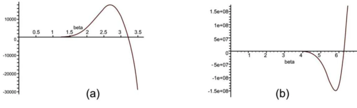
Plotting the determinant against  will give us the roots of the frequency equation for the first five natural frequencies of the cutting tool-boring bar-workpiece assembly. Figure 5 shows the first two roots.

Figure 5. The first and second roots and (a) β = 3.2 (b) β = 6.15.

The natural frequencies were calculated as shown in Table 4. The calculations were carried out taking into consideration that there are two shafts with different diameters but the same kind of material with the following properties:

, m / N , m / N

Ε 11 2 3

76036 10

2 

  d_i 0.0135m,d_ 0.01905mfor the boring

(11)

328

Table 4.The first five natural frequencies of the cutting tool-boring bar-workpiece system for model-2



n  (rad/s)

3.212 305.97

6.154 1312.14

9.401 2620.60

12.580 4692.61

15.70 7308.92

WHIRLING MOTION

Self-excited systems start to vibrate in the absence of explicit vibratory excitation force. The vibrations are caused by a source of power that is constant; however, the mechanical system converts this into an alternating source and makes the oscillations grow larger, but with some damping effect this motion is limited to finite values. In this study a displacement excitation was assumed, acting at the interaction point between the boring bar and the workpiece system. This displacement excitation is acting on the interaction point and rotating at the same time. This is illustrated in Figures 6-8. The new approach for model-1 and model-2 will be applied and simulated for both models.

Figure 6. The displacement excitation ΰ

 

t at the interaction point for model-1

(12)

329

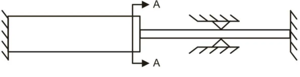
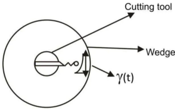
Figure 8. Section (A-A), a representation of the displacement excitationΰ

 

t

At the contact point between the boring tool (the cutting head) and the workpiece we can show that this displacement during drilling process, in addition to the shear force, is of a fluctuating increment and of dynamic origin, and the excitation that produces the latter comes from within the system, as shown in Figure 8. This displacement excitation will be concentrated and acting at the points x = xj , and hence we will use the spatial Dirac delta function:









0





1

0

 

 



x where x x at x x and



x x dx

x

L

j j

j

j  

 (35)

so that the work done at the interaction point will be equal to the shear force multiplied by the displacement and multiplied by spatial Dirac delta and it will come into play in the potential energy of the system. The dynamic loading during drilling is due to many factors, including the inherent action of the drilling process, the variation of boring bar stiffness and the wear changes of the pads. The mathematical modelling of this problem will be done using the assumed mode method, which is a procedure for the discretization of the distributed-parameter system. In the assumed mode method, the solution is assumed in the form of a finite series of space-dependent admissible functions, but the coefficients are time-dependent generalized coordinates instead of being constant. For model-1 these are assumed in the form:

 

x,t

   

x q t W

 

x,t

   

x q t

W _i

n

r i

i i

r

i



  

 

1 2 2

1 1

1  ;  (36)

where q_i

  

t  q₁,q₂,,q_r,q_r_₁,q_r_₂,,q_i



, and r is at the interaction point between the cutting head and the workpiece. The functions _i₁

   

x ,₂_i x are admissible functions, which satisfy at least the geometrical boundary conditions and q_i

 

t are the generalized coordinates. This series is substituted in the kinetic and potential energy expressions, thus reducing them to discrete form, and the equations of motion are derived by means

of Lagrange’s equations; taking into consideration that there are two distinct regions of

the boring bar-workpiece assembly, and two mode shapes for them. We assume the following for model-2:

 

x,t

   

x q t ,W

 

x,t

   

x q t andW

 

x,t

   

x q t

W _i

n

r i

i i

r

i i i

r

i



  



 



1 3 3

1 2 2

1 1

1   

(13)

330

The expressions for the kinetic and potential energies for model-1:

 

dx

t W m 2 1 dx Ω Ι 2 1 dx t W m 2 1 t , x Τ 2 2 L 0 w 2 L 0 x 2 1 L 0 b 2 1 1                    



(38)

 

L ,t ΰ

 

t W ΕΙ dx x W ΕΙ 2 1 dx x W ΕΙ 2 1 t , x V y 2 ' ' ' 2 2 2 L 0 2 2 2 2 2 L 0 2 1 2 1 2 1                    

_

(39)

 

                        





1



2

L 0 2 L 0 2 work 2 1 Bar dx t W Ceq dx t W Ceq 2 1 t , x

D (40)

The expressions for the kinetic and potential energies for model-2:

 

dx t W m 2 1 dx Ω Ι 2 1 dx Ω Ι 2 1 dx t W m 2 1 dx t W m 2 1 t , x Τ 2 L 0 w 2 L 0 x 2 L 0 x 2 L 0 b 2 1 L 0 b 1 1                              



3 2 3 2 2 (41)

 

L ,t ΰ

 

t W ΕΙ dx x W ΕΙ 2 1 d x W ΕΙ 2 1 dx x W ΕΙ 2 1 t , x V y ' ' ' 2 L 0 2 2 2 2 L 0 2 2 1 2 L 0 2 1 2 1 1                             

_

3 3 3 3 2 3 2 (42)

 

                                         





dx

t W Ceq dx t W dx t W Ceq 2 1 t , x D 2 L 0 work L 0 L 0 2 2 1 Bar

1 2 3

3

2 ₍₄₃₎

where

mb : mass per unit length of the cutting tool-boring bar assembly [Kg/m].

mw= mass per unit length of workpiece [Kg/m].

: the angular velocity of the boring bar assembly [rad/sec].

x

 : mass moment of inertia of the cutting tool-boring system about the axis of symmetry [Kg-m2].

We will proceed in the analysis for model-1 and the same is done for model-2. Applying

Lagrange’s equations on Eqns. (37-39):

Y i i Q q D q V q q dt d _                    1 1 

(14)

331 we obtain the following:

 





 2

   



 

0

            

j y 2 r 2 ij j ij j

ij q C q K ΕΙ ς L ΰ t q

Μ   (45)

where ΰ_y

 

t Displacement excitation in theY direction,

knowing that

n 1,2,..., j

i, , k

ς ς

, k

ς ς

n, 1,2,..., j

i, , ij

ς ς

, m

ς

ς ₂''_i ij

L 0

'' j 2 ij L

0 ''

i 1 ''

j 1 '

i 2 L 0

' j 2 ij L

0 '

i 1 '

j 1

1 1

m

   



 





2 2 (46)

where the (*) is for the workpiece. Now, if we take the Z direction, the boundary conditions are the same as in the Y direction. All the steps done before for the Y direction are repeated for the Z direction. For model-1, the response in the Z direction is assumed in the form of

 

x,t

   

x F t R

 

x,t

   

x F t

R _i

n

r i

i i

r

i



  

 

1 2 2

1 1

1  ;  (47)

For model-2, the response in the Z direction is assumed in the form of

 

x,t

     

x F t R x,t

     

x F t R x,t

   

x F t

R _i

n

r i

i i

r

i i i

r

i



  



 



1 3 3

1 2 2

1 1

1  ;  ;  (48)

The functions _i₁

   

x ,₂_i x are admissible functions and F_i

 

t are the generalized coordinates. Assuming the displacement excitation in the Z direction as

 

t

γZ , and using the same expressions for the kinetic, potential and dissipation energies

as in the Ydirection and applying Lagrange’s equations in the Z direction, we obtain the following expressions:

 





 ₂

   



 

0

            

j y 2 r 2 ij j

ij j

ij F C F K ΕΙ ς L ΰ t F

Μ   ₍₄₉₎

where ΰ_z

 

t Displacement excitation in theZ direction. Eq. (45 and Eq. (49) are subject to the following constraint: W₂

 

L₂,t W₁

   

L₁,t  t and

 

L ,t R

   

L,t ΰt

R₂ ₂  ₁ ₁  . For model-2 we have the following constraint:

 

L ,t W

   

L,t t

(15)

332

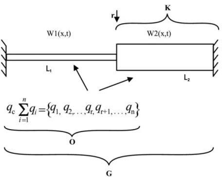
Figure 9. The boring bar–workpiece system; O and K are subsystems of G.

The equations were derived depending upon the constraint of the problem as follows:



r r n



n

i i

c q q ,q , ,q ,q , ,q

q ₁ ₂  ₁ 

1    







   

 

     

 

     

   

 

   

 

t q

 

t q

 

t C



q

 

t q

 

t q

 

t



C ΰ

 

t

q t ΰ C t q C t q t ΰ L ς 1 t q L ς L ς t q t ΰ t q L ς t q L ς t ΰ t q L ς t q L ς t ΰ t q L ς t q L ς t ΰ t , L W t , L W 2 n 2 r 1 r 1 r 2 1 2 n 1 r 1 r 1 r 1 i i 1 r 1 i 1 i 1 r r 1 i 1 1 i n 1 r 2 2 1 r r 1 i i 1 r n 1 r 2 2 1 r i r 1 i 2 1 i i r 1 i 2 1 i 1 r n 1 r 2 2 1 r i r 1 i 2 1 i 1 r n 1 r 2 2 1 r 1 1 2 2                                                                                 



Now if we choose to drop q_r_₁

 

t and replace it by q_r

 

t , we will have the following:

 

ΰ

 

t C C t q 1 C 1 t q t ΰ C t q t q C t ΰ C t q C t q 1 2 r 1 r 2 r 1 r 1 2 1 r 1

r        



(16)

333 From the main equation,

 



   



0

1 2 1 2 1 2 1 1 2 1                                                                          n r r y 2 ' ' ' r 2 ij n r r ij n r r ij q q q q q t ΰ L ς ΕΙ K q q q q q C q q q q q Μ                     

The generalized coordinates of the whole system



r r n



n

i i

c q q ,q , ,q ,q , ,q

q ₁ ₂  ₁

1

 

 



and we choose the general coordinate q_r_₁

 

t :

 q

 

t C q

 

t



K  ΕΙ ς

   

L ΰ t



q

 

t 0.0

Mijatr1r1  ijatr1r1  ijatr1 2 r2 2 y r1 

Knowing that

 

ΰ

 

t C C t q 1 C 1 t q 1 2 r 1

r  



 _   , we substitute this in the above equation:

 

   





 

ΰ

 

t 0.0

C C t q 1 C 1 t ΰ L ς ΕΙ K t ΰ C C t q 1 C 1 C t ΰ C C t q 1 C 1 M 1 2 r y 2 2 r 2 1 r at ij 1 2 r 1 r at ij 1 2 r 1 r at ij                                           

 



 

   



 





 



 

   



 



M ΰ t C ΰt K ΕΙ ς L ΰ t ΰ t



C C t q t ΰ L ς ΕΙ K t q C t q M C 1 y 2 2 r 2 1 r at ij 1 r at ij 1 r at ij 1 2 r y 2 2 r 2 1 r at ij r 1 r at ij r 1 r at ij 1                      or  

 



 

   



 





 



 

   



 



M ΰ t C ΰt K ΕΙ ς L ΰ t ΰ t



C t q t ΰ L ς ΕΙ K t q C t q M y 2 2 r 2 1 r at ij 1 r at ij 1 r at ij 2 r y 2 r 2 1 r at ij r 1 r at ij r 1 r at ij                      ₂

The two equations of motion will be

   

 

t C ΰ

 

t



K ΕΙ ς

   

L ΰ t



ΰ

 

t )

ΰ (M C q ] t ΰ L ς ΕΙ K [ q C q Μ y y 2 r 2 y 11 y 11 1 y 2 12 2 11 1 11 1 11 2 11

2    

           (50)

   

 

t C ΰ

 

t



K ΕΙ ς

   

L ΰ t

  

ΰ t )

ΰ (M C F ] t ΰ L ς ΕΙ K [ F C F Μ z z 2 r 2 z 11 z 11 1 Z 2 12 2 11 1 11 1 11 2 11

2    

(17)

334 where C2 =

 

1 11

1

L

 Since the excitation displacement is rotating, Eq. (50) and Eq. (51) will be as follows:

   

 

t C ΰ

 

t



K ΕΙ ς

   

L ΰ t



ΰ

 

t )cosΩt ΰ

(M C

q ]

Ωt

cos t

ΰ

L

ς ΕΙ

K [ q C q

Μ

y y 2 r 2 y

11 y

11

1 y

2 2 11 1

11 11

2 11

12 1

   



 

 



 

  



(52)

     

 

t C ΰ

 

t



K ΕΙ ς

   

L ΰ t

  

ΰ t )sin

 

Ωt ΰ

(M C

F ]

Ωt

sin t

ΰ

L

ς ΕΙ

K [ F C F

Μ

z z 2 r 2 z

11 z

11

1 Z

2 12 2 11 1

11 1 11

2 11 

 



 

 



 

  



(53)

Now we will assume that the fundamental component of displacement excitation function is in the form of ΰ_y

 

t __y sin

 

t and ΰ_Z

 

t __z sin

 

t , where : is the frequency of the wedge excitation as it is introduced back and forth at the interaction point and rotating at the same time. We will use the following relations:

   

sin



2Ωt



2

1 t

Ω

cos t

θ

sin  , at  (54)

   



1 cos



2Ωt



2

1 t

Ω

sin t

θ

sin   , at  (55)

   



sin



θ Ω



t sin



θ Ω



t



2

1 t

Ω

cos t

θ

sin     , at  (56)

   



cos



θ Ω



t cos



θ Ω



t



2

1 t

Ω

sin t

θ

sin     ,  (57)

If  , the rotation frequency is equal to the wedge excitation frequency, and we use Eq. (49) and Eq. (50). When  we use Eq. (51).

We have two cases to simulate: the first when the rotation frequency is equal to the wedge excitation frequency and the second when the rotation frequency is not equal to the wedge excitation frequency. The following numerical values and relations were used in the calculation:

m L , m . L , m .

d , m .

d , m / N ,

m /

N 76036 i 00135 001905 25 1

10

2 1 2

3 2

11     

 

  _









2

2 4

2 2 2 1

4 4 1

4 64

4

64 d di and A d di , dw and A dw

 

 

 

 



 _ _

The simulation results for model-1 are shown in Figure 10. Figure 10 (a) is a general scale figure, while Figures 10 (b, c, d, e) are at 0.25L1, 0.5L1, 0.75L1 and L1,

respectively. Figure 10 (f) is at = first natural frequency of the boring bar.

(18)

335

Figure 10. Whirl orbit of the shaft at  =20(Hz), 0y = 3.18E-04 m and 0z

=3.39E-04 m at: (a) General scale figure, (b) 0.25 L1, (c) 0.5 L1, (d) 0.75 L1,(e) L1 and (f) 1st

natural frequency.

Figure 11. Whirl orbit of the shaft when  (20 Hz , 5Hz), 0y = 3.18E-04

m and 0z =3.39E-04 m.

EXPERIMENTAL RESULTS OF WHIRLING MOTION

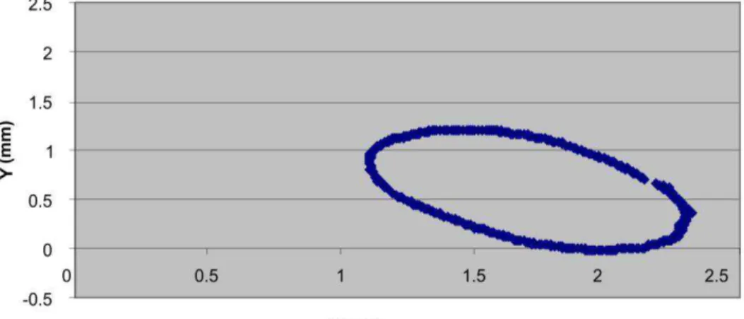
The experiments will include investigation of the whirl orbits of the boring bar–cutting head assembly while rotating at a speed of 1280 rpm, as shown in Figure 12. It is obvious from this Figure that the whirling motion is tilted and inclined and rotating around the geometric axis as the mathematical mode predicted.

(19)

336

given periodic function in terms of cosine and sine functions. As seen in Figure 13, at speeds of 1200, 1280, 1359 and 1440 rpm the power spectral density, PSD, is the amount of power per unit (density) of frequency (spectral) and describes how the power (or variance) of a process is distributed with frequency.

Figure 12. A sample of the whirling orbit resulting from an experiment at speed of 1280 rpm.

An equivalent definition of PSD is the squared modulus of the Fourier transform of the time series. Recalling the Fourier transform for a continuous Fourier time series, the power spectral density S(f) for a discrete Fourier transform is defined as

 

* N N Nlim _T F F

f

S  

 

1

(59)

where the star symbol denotes complex conjugate. In Figure 13, we have four main spectral peaks in this figure which correspond to the fundamental frequency. The other spectral peaks corresponds to the 2nd, 3rd, 4th, etc., natural frequencies of the system.

100 101 102 103

10-9 10-8 10-7 10-6 10-5 10-4 10-3 10-2

Frequency (Hz)

P

S

D

(

m

2)

1200 rpm 1280 rpm 1359 rpm 1440 rpm

(20)

337

INSTANTANEOUS LOCATION OF THE BORING BAR CENTRE WITH RESPECT TO THE GEOMETRIC CENTRE WHILE ROTATING

Whirl is defined as the locus of the instantaneous centre of rotation of the rotating shaft. Under different speeds of rotation the boring bar will have different positions with respect to the geometric centre of the drilled holes. We investigated this location for eight speeds. The geometric centres under zero rotation and different speeds of rotation 1200 and 1440 rpm are shown in Figure 14.

Figure 14. Two monitored tilted centres of the boring bar at speeds of 1200 and 1440 rpm.

The constant drive for higher accuracy, surface finish and at the same time higher productivity to withstand the economic competition has led to many improvements in cutting tools and cutting methods. Considering the amount of hole production in a manufacturing activity, the quest for better drilling tools and procedures is always at the forefront of such drives. The type of hole making operation selected usually depends upon the following hole requirements: diameter of the hole; depth of the hole; quality of the hole surface; size, accuracy, parallelism and straightness. Machining holes of high length-to-diameter ratios to high standards of size, parallelism, straightness and surface finish has always presented a problem, since hole straightness deteriorates when the hole length to diameter ratio exceeds three. As seen in Figure 14, the tool is oscillating due to a whirling motion around the bored surface, and these oscillations contain many harmonies and cause surface irregularities.

CONCLUSIONS

(21)

338

 Whirling motion is a self-excited vibration and can be reduced but not eliminated and the high length of the boring bar relative to its diameter caused the whirling motion.

 When the length of the boring bar increased, an initial deflection of the boring bar could be a natural cause and an initiator of the whirling motion which is sustained while drilling.

 The mathematical model mimics the actual behaviour of the real system in terms of the whirling ellipse and the tilted motion.

 The fundamental frequency value of the analytical model is close to the value of the real system.

 The whirling motion of the boring bar is a forward whirling motion, where the direction of the whirling motion is in the same direction as the boring bar rotation.

 The oscillation of the tool around the bored surface causes bad surface properties, so future work will study the effect of the whirling motion at the beginning of drilling under different speeds of rotation and the effect of changing cutting parameters on the whirling motion which affects the surface irregularities.

ACKNOWLEDGEMENT

The author would like to thank the Al-Huson University College and Al-Balqa’Applied University management for their continuous support and guidance in all our research activities. Also, potential collaboration with Swinburne University of Technology (Sarawak Campus) is highly appreciated.

REFERENCES

Batzer, S.A., Gouskov, A.M. and Vornov, S.A. 2001. Modeling vibratory drilling dynamics. Transactions of ASME, Journal of Vibration and Acoustics, 123(4): 435-443.

Bayly, P.V., Lamar, M.T. and Calvert, S.G. 2002. Low-frequency regenerative vibration and the formation of lobed holes in drilling. Transactions of ASME, Journal of

Manufacturing Science and Engineering, 124: 275-285.

Bayly, P.V., Metzler, S.A., Schaut A.J. and Young, K.A. 2001. Theory of tensional chatter in twist drills: model, stability analysis and composition to test.

Transactions of ASME, Journal of Manufacturing Science and Engineering,

123: 552-561.

Bayly, P.V., Young, K.A., Calvert, S.G. and Hally, J.E. 2001. Analysis of tool oscillation and hole roundness error in a quasi-static model of reaming.

Transactions of ASME, Journal of Manufacturing Science and Engineering,

123: 387-396.

Chandrashekhar, S. 1984. An analytical and experimental stochastic modeling of the resultant force system in BTA deep-hole machining and its influence on the

dynamics of the machine tool workpiece system. PhD Thesis, Concordia

University, Canada.

Ema, S., Fujii, H. and Marui, E. 1988. Chatter vibration in drilling. Transactions of