A new estimation of the recent tropospheric molecular hydrogen budget using atmospheric observations and variational inversion

(1)

ACPD

10, 28963–29005, 2010

H₂ 4D-var

C. Yver et al.

Title Page

Abstract Introduction

Conclusions References

Tables Figures

◭ ◮

Back Close

Full Screen / Esc

Printer-friendly Version Interactive Discussion

Discussion

P

a

per

|

Dis

cussion

P

a

per

|

Discussion

P

a

per

|

Discussio

n

P

a

per

|

Atmos. Chem. Phys. Discuss., 10, 28963–29005, 2010 www.atmos-chem-phys-discuss.net/10/28963/2010/ doi:10.5194/acpd-10-28963-2010

Atmospheric Chemistry and Physics Discussions

This discussion paper is/has been under review for the journal Atmospheric Chemistry and Physics (ACP). Please refer to the corresponding final paper in ACP if available.

A new estimation of the recent

tropospheric molecular hydrogen budget

using atmospheric observations and

variational inversion

C. Yver1, I. Pison1,2, A. Fortems-Cheiney1, M. Schmidt1, P. Bousquet1,2,

M. Ramonet1, A. Jordan3, A. Søvde4, A. Engel5, R. Fisher6, D. Lowry6, E. Nisbet6, I. Levin7, S. Hammer7, J. Necki8, J. Bartyzel8, S. Reimann9, M. K. Vollmer9, M. Steinbacher9, T. Aalto10, M. Maione11, I. Arduini11, S. O’Doherty12, A. Grant12, W. Sturges13, C. R. Lunder14, V. Privalov15, and N. Paramonova15

1

Laboratoire des Sciences du Climat et de l’Environnement (LSCE), UMR 8212, Gif sur Yvette, France

2

Universit ´e de Versailles Saint Quentin en Yvelines (UVSQ), Versailles, France

3

Max Planck Institut f ¨ur Biogeochemistry, 07701 Jena, Germany

4

(2)

ACPD

10, 28963–29005, 2010

H₂ 4D-var

C. Yver et al.

Title Page

Tables Figures

◭ ◮

Back Close

Full Screen / Esc

Discussion

P

a

per

|

Dis

cussion

P

a

per

|

Discussion

P

a

per

|

Discussio

n

P

a

per

|

5

Institut f ¨ur Meteorologie und Geophysik, Johann Wolfgang Goethe-Universit ¨at Frankfurt, Frankfurt, Germany

6

Department of Geology, Royal Holloway, University of London, Egham, UK

7

Institut f ¨ur Umweltphysik, University of Heidelberg, Heidelberg, Germany

8

Faculty of Physics and Applied Computer Science, AGH-University of Science and Technology, 30-059 Krakow, Al. Mickiewicza 30, Poland

9

Empa, Swiss Federal Institute for Materials Science and Technology, Laboratory for Air Pollution/Environmental Technology, Ueberlandstrasse 129, 8600 Duebendorf, Switzerland

10

Finnish Meteorological Institute, Climate Change Research, P.O. Box 503, 00101 Helsinki, Finland

11

Universit `a degli Studi di Urbino, Istituto di Scienze Chimiche, Piazza Rinascimento 6, 61029 Urbino, Italy

12

School of Chemistry, University of Bristol, UK

13

School of Environmental Sciences, University of East Anglia, Norwich, UK

14

Norwegian Institute for Air Research, P.O. Box 100, 2027 Kjeller, Norway

15

Voeikov Main Geophysical Observatory, St. Petersburg, Russia

Received: 18 October 2010 – Accepted: 18 November 2010 – Published: 25 November 2010

Correspondence to: C. Yver ([email protected])

(3)

ACPD

10, 28963–29005, 2010

H₂ 4D-var

C. Yver et al.

Title Page

Tables Figures

◭ ◮

Back Close

Full Screen / Esc

Discussion

P

a

per

|

Dis

cussion

P

a

per

|

Discussion

P

a

per

|

Discussio

n

P

a

per

|

Abstract

This paper presents an analysis of the recent tropospheric molecular hydrogen (H2)

budget with a particular focus on soil uptake and surface emissions. A variational inversion scheme is combined with observations from the RAMCES and EUROHY-DROS atmospheric networks, which include continuous measurements performed

be-5

tween mid-2006 and mid-2009. Net H2 surface flux, soil uptake distinct from surface

emissions and finally, soil uptake, biomass burning, anthropogenic emissions and N₂ fixation-related emissions separately were inverted in several scenarios. The various inversions generate an estimate for each term of the H2 budget. The net H2 flux per

region (High Northern Hemisphere, Tropics and High Southern Hemisphere) varies

be-10

tween−_{8 and 8 Tg yr}−1_{. The best inversion in terms of fit to the observations combines}

updated prior surface emissions and a soil deposition velocity map that is based on soil uptake measurements. Our estimate of global H2soil uptake is−59±4.0 Tg yr

−1

. Forty per cent of this uptake is located in the High Northern Hemisphere and 55% is located in the Tropics. In terms of surface emissions, seasonality is mainly driven by

15

biomass burning emissions. The inferred European anthropogenic emissions are con-sistent with independent H₂ emissions estimated using a H₂/CO mass ratio of 0.034 and CO emissions considering their respective uncertainties. To constrain a more robust partition of H2 sources and sinks would need additional constraints, such as

isotopic measurements.

20

1 Introduction

With a mixing ratio of about 530 ppb (part-per-billion, 10−9), tropospheric H2 is the

second most abundant reduced trace gas in the troposphere after methane (CH₄). In

contrast to CH4and other trace gases sharing anthropogenic sources, the observed H2

mixing ratios are lower in the Northern Hemisphere when compared to the Southern

25

(4)

ACPD

10, 28963–29005, 2010

H₂ 4D-var

C. Yver et al.

Title Page

Tables Figures

◭ ◮

Back Close

Full Screen / Esc

Discussion

P

a

per

|

Dis

cussion

P

a

per

|

Discussion

P

a

per

|

Discussio

n

P

a

per

|

The mean strength of each term of the H2 budget is given hereafter as referred to in

the literature (Novelli et al., 1999; Hauglustaine and Ehhalt, 2002; Sanderson et al., 2003; Xiao et al., 2007; Price et al., 2007; Ehhalt, 2009). The main sources of H2 are

photochemical production by the transformation of formaldehyde (HCHO) in the atmo-sphere and incomplete combustion processes. Photolysis of HCHO, a product in the

5

oxidation chain of methane and other volatile organic compounds (VOCs) accounts for 31 to 77 Tg yr−1 and represents half of the total H2 source. Fossil fuel and biomass

burning emissions, two incomplete combustion sources, account for similar shares of the global H2budget (10–23 Tg yr

−1

, or 20% each). Minor H2emissions originate from

nitrogen fixation in the continental and marine biosphere and complete the sources (6–

10

11 Tg yr−1). H₂oxidation by free hydroxyl radicals (OH) and enzymatic H₂destruction in soils must balance these sources because tropospheric H2does not show a

signif-icant long term trend (Grant et al., 2010b). H2 oxidation through OH accounts for 8

to 25 Tg yr−1, which is equivalent to 20% to 30% of the total H₂ sink. H₂ soil uptake, the major sink in the budget (65 to 105 Tg yr−1or 70% to 80% of the total sink), is

re-15

sponsible for the observed latitudinal surface gradient. It is, however, relatively poorly constrained due to uncertainties regarding its associated physical and chemical pro-cesses. Specifically, H₂ uptake is driven by enzymatic and microbial activities linked to H2 diffusivity, which depend mostly on soil moisture and temperature (Conrad and

Seiler, 1981, 1985; Yonemura et al., 1999, 2000a,b; Lallo et al., 2008, 2009; Schmitt

20

et al., 2009).

Although global studies of H2 mixing ratios using observations from sampling

net-works began in the 1990s, Schmidt (1978) had already presented meridional profiles of the Atlantic Ocean from ship cruise measurements. Subsequently, Khalil and

Ras-mussen (1990) announced an increase in H2 mean mixing ratio based on weekly

25

samplings between 1985 and 1989 at six locations from 71.5◦N to 71.4◦S. Novelli

(5)

ACPD

10, 28963–29005, 2010

H₂ 4D-var

C. Yver et al.

Title Page

Tables Figures

◭ ◮

Back Close

Full Screen / Esc

Discussion

P

a

per

|

Dis

cussion

P

a

per

|

Discussion

P

a

per

|

Discussio

n

P

a

per

|

with oceanic samplings and Antarctic sites. This network has been running for H2

since 1989 with regards to the first sites and was extended progressively to include all of the 52 sites in 1994. The CSIRO Global Flask Sampling Network (ten stations) began sampling in 1992 with a larger focus on the Southern Hemisphere (Langenfelds et al., 2002). Finally, within the AGAGE programme (Advanced Global Atmospheric

5

Gases Experiment), H2 has been measured continuously since 1993 at two stations

worldwide (Prinn et al., 2000). A small increasing trend was extracted from the anal-ysis of the observations provided by the NOAA network (Novelli et al., 1999) whereas the CSIRO observations exhibited a small decrease (Langenfelds et al., 2002). Since

2006, in the frame of the European project EUROHYDROS, a H2monitoring network,

10

focusing mainly on Europe (13 continuous and 5 flask sampling sites) but also world-wide through 10 flask sampling sites outside Europe, was developed (Engel, 2009). The French Atmospheric Network for Greenhouse Gases Monitoring (RAMCES), part of the Laboratory for Climate and Environmental Sciences (LSCE) has provided ob-servations from 10 sites (one of them sampling continuously) to the EUROHYDROS

15

network and contributed with nine additional sites to this study. Parallel to the obser-vations, forward modelling studies were used to provide the first constraints on the H₂ budget (Hauglustaine and Ehhalt, 2002; Price et al., 2007). Nevertheless, since the soil sink, the major loss term, is only known with large uncertainties, it is represented in models with more or less simplified assumptions which lead to a wide range of

es-20

timations for every term of the budget and especially for the soil sink, ranging from 40 to 90 Tg yr−1(Ehhalt, 2009).

Atmospheric observations combined with a chemistry-transport model and prior in-formation on surface fluxes and sources and sinks within the atmosphere allow (in a Bayesian inversion framework) to retrieve the estimations of the H2sources and sinks

25

and their uncertainties. Atmospheric inversions have already been developed to study H2, but the studies remain sparse: Xiao et al. (2007) have used a 2-D latitude-vertical

(6)

ACPD

10, 28963–29005, 2010

H₂ 4D-var

C. Yver et al.

Title Page

Tables Figures

◭ ◮

Back Close

Full Screen / Esc

Discussion

P

a

per

|

Dis

cussion

P

a

per

|

Discussion

P

a

per

|

Discussio

n

P

a

per

|

of H2sources and sinks for four semi-hemispheres over the 1993–2004 period. More

recently, Bousquet et al. (2010) have provided an analysis of global-to-regional details in the H2 budget before 2005 based on large regions, using a synthesis inversion, a

3-D chemistry transport model and discrete observations from the flask networks of NOAA and CSIRO.

5

In this paper, we present the mixing ratio measurements of the RAMCES and EU-ROHYDROS sampling networks (13 continuous stations and 25 flasks sampling sites) for H₂since January 2005. These time series provide information on seasonal cycles and H2 distribution with latitude. As no NOAA data were available for this period, we

have chosen to use only the data from the RAMCES and EUROHYDROS networks.

10

The observations from mid-2006 to mid-2009 are assimilated in a variational inversion to estimate the global H2budget. Contrary to Bousquet et al. (2010), the observations

are continuous as well as discrete, from a more recent period and they are centred on Europe. Six di_fferent scenarios have been elaborated to progressively constrain the terms of the H2 budget. The results, with a detailed analysis of Europe (where 27 of

15

the 38 sites are located), are presented below.

2 Observational network

2.1 RAMCES flask sampling network

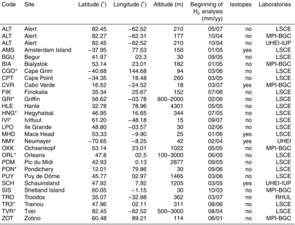
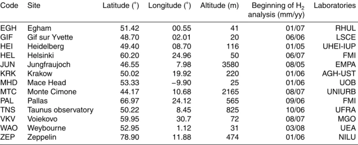
RAMCES network’s central laboratory is located at Gif-sur-Yvette (GIF) near Paris, France. During the period between 2006 and 2009, the RAMCES network analysed air

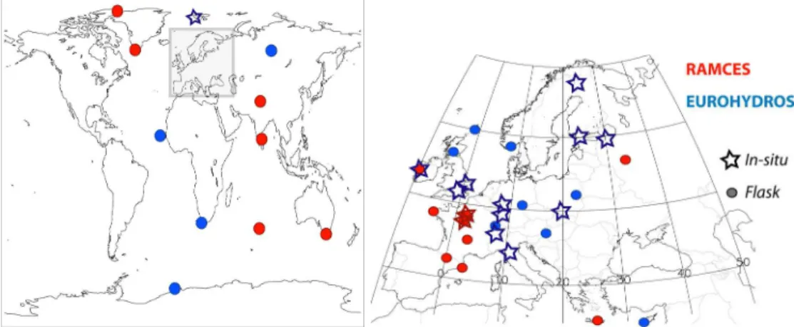
20

from 19 sampling sites in the world (see Fig. 1). At eighteen sites, flasks were sampled weekly or biweekly. At all of the sites except Ivvittut (Greenland) site, flask sampling began before the H2 analyser was installed in the central laboratory of Gif-sur-Yvette

to monitor other greenhouse gases (CO2, CH4, N2O, SF6, CO). At Gif-sur-Yvette, air is

sampled continuously. Table 2 lists the RAMCES flask network sites used in this study

25

(7)

ACPD

10, 28963–29005, 2010

H₂ 4D-var

C. Yver et al.

Title Page

Tables Figures

◭ ◮

Back Close

Full Screen / Esc

Discussion

P

a

per

|

Dis

cussion

P

a

per

|

Discussion

P

a

per

|

Discussio

n

P

a

per

|

They are distributed across latitudes from 40◦S to 82◦N and, for most of them, they provide access to background air that is representative of zonal mean atmospheric composition. At the sites of Tver (Russia), Hegyhatsal (Hungary), Griffin (Scottland) and Orl ´eans (France), monthly to weekly light aircraft flights have sampled the tro-posphere between 100 and 3000 m. These sites were part of the CARBOEUROPE

5

programme that ended in December 2008. Trainou (France), Puy de D ˆome (France), Pic du Midi (France) and Hanle (India) are situated inland but, except for Trainou, which regularly encounters polluted air masses, they are situated at high altitude and away from local anthropogenic influences. All of the other ground sites are coastal and they encounter air masses characterized by long marine back-trajectories.

10

2.2 EUROHYDROS network

In the EUROHYDROS project (September 2006 to September 2009), twenty labora-tories from ten different countries participated. In this study, atmospheric H2

mea-surements at 31 sites performed by 13 laboratories running over the period 2006 to 2009, are used in the variational inversion (see Table 1, Table 2 and Fig. 1). At 13

15

sites, ambient air is continuously sampled. For three stations (Alert (Canada), Mace Head (Ireland) and Bialystok (Poland)), simultaneous sampling by di_fferent laboratories is performed. Seven stations (Egham (UK), Gif-sur-Yvette (France), Heidelberg (Ger-many), Helsinki (Finland), Krakow (Poland), Tver and Voiekovo (Russia)) sample air in urban or suburban conditions. Continental sites such as Trainou (France) or

Schauins-20

land (Germany) encounter alternatively clean and moderately polluted air masses. At Mace Head, Finokalia (Greece), Troodos (Cyprus) and Begur (Spain), the sampled air is under clean maritime and moderately polluted influences. The remaining stations mainly encounter clean background air. For six sites (Alert, Mace Head, Schauinsland, Cabo Verde, Amsterdam Island and Neumayer (Antarctica)), hydrogen isotopes in the

25

sampled flasks are analysed by the University of Utrecht.

During the project, H2soil deposition velocities were measured at different sites and

(8)

ACPD

10, 28963–29005, 2010

H₂ 4D-var

C. Yver et al.

Title Page

Tables Figures

◭ ◮

Back Close

Full Screen / Esc

Discussion

P

a

per

|

Dis

cussion

P

a

per

|

Discussion

P

a

per

|

Discussio

n

P

a

per

|

2009; Yver et al., 2009; Schillert, 2010). Theses flux estimations were interpolated into a soil uptake map as detailed in Sect. 3.3.

2.3 Sampling technique

In the frame of the EUROHYDROS project, all laboratories were requested to follow the recommendation for good measurement practice, a protocol developed at the

begin-5

ning of the project (Engel, 2009). The calibration and non-linearity correction strategy, the type of standard gas cylinders, pressure regulators and instrumental set-up were specified there. In particular, all the samples were measured using standard cylinders calibrated against the MPI2009 scale, which has been elaborated for the EUROHY-DROS project (Jordan, 2007; Jordan and Steinberg, 2010).

10

Within the RAMCES network, we followed this strategy as described in detail by Yver et al. (2009). Briefly, a commercial gas chromatograph coupled with a reduction gas detector (RGD) from Peak Laboratories, Inc., California, USA is used to measure

H₂ via the reduction of mercuric oxide and the detection of mercury vapour by UV

absorption. Sixteen inlet ports are set up on a 16-port Valco valve to connect flask

15

samples to the inlet system. To avoid contamination and reduce the flushing volume of the sample when measuring the flasks, all sample inlet lines can be separately evacuated. Pairs of flasks are sampled at the sites as a rule, to check for sampling error or any malfunction in the sampling equipment. Each flask is then analysed twice to check the reproducibility of the measurements. Statistics on pair and double injection

20

analyses give a reproducibility below 1% (≈_{3 ppb).}

The analysis technique for atmospheric H2within the EUROHYDROS network is for

most of the laboratories also based on the separation with gas chromatography and the detection with a RGD. The methods, following the recommendation for good mea-surement practice, are described for some of the laboratories in the following papers:

25

(9)

ACPD

10, 28963–29005, 2010

H₂ 4D-var

C. Yver et al.

Title Page

Tables Figures

◭ ◮

Back Close

Full Screen / Esc

Discussion

P

a

per

|

Dis

cussion

P

a

per

|

Discussion

P

a

per

|

Discussio

n

P

a

per

|

To ensure the compatibility of the data of the different laboratories, regular calibra-tion against the common scale but also comparison of measurements done at the same site (Alert or Mace Head for example) and comparison exercises (Star Robin and Round Robin) were performed. From these last comparisons, the agreement be-tween the 13 laboratories was better than 1.4% (Engel, 2009).

5

2.4 Observations used in the inversion

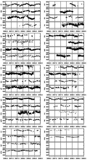
The observations from the 38 RAMCES and EUROHYDROS sites are plotted in Fig. 2. The Figure presents the sites by latitude, from the north to the south. For the con-tinuous stations, the daily means are plotted and mixing ratios above 800 ppb, which correspond to strong local pollution events, are excluded. The mean mixing ratios

10

range from≈_{500 ppb at Alert to}≈_{550 ppb at Neumayer with a maximum in the Tropics}

(≈_{570 ppb at Pondichery (India)). We observe a seasonal cycle at all of the sites but}

with a greater amplitude and deeper minima in the High Northern Hemisphere (HNH, above 30◦N). In this hemisphere, the seasonal maximum (up to 540 ppb) occurs in the

spring (April, May) and the minimum of≈_{430 ppb is observed in the autumn}

(Septem-15

ber, October). In the Northern Tropics (between 30◦N and 0◦N), the seasonal cycle is shifted by about two months (maximum July and minimum in December), whereas

in the High Southern Hemisphere (HSH,below 30◦S), the seasonal maximum occurs

in the austral summer (January, February) reaching up to 580 ppb and the minimum occurs in mid austral winter (August, September) equaling 550 ppb. The maximum

20

amplitude is found in the HNH with about 110 ppb peak-to-through and the minimum is found in the HSH with 30 ppb peak-to-through. These patterns reflect the differences in the location and timing of H2 sources and sinks. In the HSH and the Tropics, the

seasonal variations are mostly explained by the timing of biomass burning emissions and photochemical production, which peak in the summer. The higher minima than in

25

(10)

ACPD

10, 28963–29005, 2010

H₂ 4D-var

C. Yver et al.

Title Page

Tables Figures

◭ ◮

Back Close

Full Screen / Esc

Discussion

P

a

per

|

Dis

cussion

P

a

per

|

Discussion

P

a

per

|

Discussio

n

P

a

per

|

weaker compared to summer. The maximum occurs in the spring when the soil uptake is the weakest.

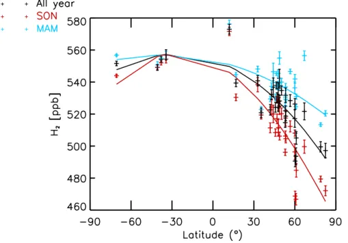
In Fig. 3, the latitudinal gradient is based on the mean mixing ratio at every site, except for the urban sites such as Heidelberg (Germany), Krakow (Poland), Egham (London suburb, UK) and Tver (Moscow suburb, Russia), where the anthropogenic

5

pollution enhances the background level of H2. As already described, the lower mixing

ratios are measured in the HNH. Mean mixing ratios show an increase with decreasing latitudes until 30◦S and then show a slight decrease from 30◦S to 70◦S. From the north to the south, the mean gradient is≈_{50 ppb and from the north to the Tropics,}

it is ≈_{60 ppb. According to our colour scheme, the latitudinal gradient is plotted in}

10

September/October/November in red and in March/April/May in blue. As expected, in the HNH, the mixing ratios are lower in the autumn than they are in the spring. The latitudinal gradient is also larger in the autumn with ≈_{70 ppb than it is in the spring}

(≈_{35 ppb).}

All of these patterns highlight the importance of the soil uptake in the spatiotemporal

15

variations of the H2 mixing ratios and the need to estimate its strength and variations

better.

3 The variational inversion system

3.1 General settings of PYVAR/LMDz-SACS

We use a framework which combines three components: the inversion system

PY-20

VAR developed by Chevallier et al. (2005), the transport model LMDzt (Hourdin and Talagrand, 2006) and a simplified chemistry module called SACS (Simplified

Atmo-spheric Chemistry System) (Pison et al., 2009). LMDzt is the off-line version of

the general circulation model (GCM) of the Laboratoire de M ´et ´eorologie Dynamique (LMDz) (Sadourny and Laval, 1984; Hourdin and Armengaud, 1999). Briefly, LMDzt is

25

(11)

ACPD

10, 28963–29005, 2010

H₂ 4D-var

C. Yver et al.

Title Page

Tables Figures

◭ ◮

Back Close

Full Screen / Esc

Discussion

P

a

per

|

Dis

cussion

P

a

per

|

Discussion

P

a

per

|

Discussio

n

P

a

per

|

resolution in the boundary layer of 300 to 500 m and ≈_{2 km at the tropopause) and}

a horizontal resolution of 3.75◦×_2.5◦ _{(longitude-latitude). The air mass fluxes used}

off-line are pre-calculated by LMDz online GCM nudged on ECMWF analysis for

hori-zontal wind. SACS is a simplified methane oxidation chain. SACS keeps only the main species and the major reactions. The intermediate reactions are regarded as very fast

5

compared to the principal reactions. In the atmosphere, the oxidation by OH is the main sink of CH4. This reaction is the first in a chain of photochemical transformations which

lead to formaldehyde which is also produced from the degradation of volatile organic compounds (VOCs) in the continental boundary layer. H2is at the end of the reaction

chain along with CO as a product of the transformation of formaldehyde:

10

HCHO+hν−→_H₂₊_CO ₍₁₎

Although OH is the essential modulator of this reaction chain, this short-lived com-pound (≈_{1 s) is not easily measurable on a global scale. Its concentration is estimated}

only in an indirect way: using methyl chloroform (CH₃CCl₃or MCF) which reacts only with OH and the sources of which are quantified with acceptable accuracy (Krol et al.,

15

2003; Prinn et al., 2005; Bousquet et al., 2005). The adequacy of SACS with the full chemistry-transport model LMDz-INCA is evaluated in Pison et al. (2009). These authors show that the differences between the two chemistry models are significantly smaller than the variability of the concentration fields of the species of interest. To obtain the initial conditions for the simulations with SACS, the full chemistry-transport

20

model LMDz-INCA is used to establish fields of OH and VOCs that are consistent with the initial state of the system (Hauglustaine et al., 2004). The deposition velocities for

H₂, reaction constants and photolysis rates are also given to PYVAR by LMDz-INCA

(Hauglustaine and Ehhalt, 2002). SACS can be used to estimate the sources and sinks of CH4, CO, HCHO and H2. In this work, we focus on only H2and the fluxes of CO and

25

CH4 are assumed to have been optimised and their errors are set to ±1%, whereas

(12)

ACPD

10, 28963–29005, 2010

H₂ 4D-var

C. Yver et al.

Title Page

Tables Figures

◭ ◮

Back Close

Full Screen / Esc

Discussion

P

a

per

|

Dis

cussion

P

a

per

|

Discussion

P

a

per

|

Discussio

n

P

a

per

|

PYVAR is a Bayesian inference scheme formulated in a variational framework. It consists in the minimisation of a cost functionJ(x):

J₍x)=(x−xb)

T

B−1(x−xb)+(H(x)−y) T

R−1(H₍_x₎−_y₎ ₍₂₎

wherexis the state vector containing the variables that need to be estimated at each model grid cell, xb contains the prior values of the variables and y the observations

5

andH _{is the operator representing the chemistry-transport model and the retrieval of}

the equivalent of the observations. B and R are the covariance matrices of the

er-ror statistics ofxb and y, respectively. The state vector contains the emission fluxes

(here for H2) and the average production of HCHO in each cell at eight-day frequency,

the average OH concentrations as described by Bousquet et al. (2005) (four latitudinal

10

bands) at the same frequency and the initial conditions for the concentrations (here of H2). The system finds the optimalxa which fits the observations and the prior values

as weighted by the covariance matricesRand B. Physical considerations as detailed in Chevallier et al. (2005), are used to infer the errors (variances, spatial and temporal correlations) of the prior. In this study, the errors are set to±_{100% of the maximal}

15

flux in the grid cell over the inversion period for H₂, 1% of the flux for MCF (in order to constrain OH), CO, CH4and HCHO fluxes. The error of±10% for OH concentrations is

consistent with the differences between estimates of the OH concentrations of several studies (Krol et al., 2003; Prinn et al., 2005; Bousquet et al., 2005). Finally, the error

on the initial concentrations of HCHO, MCF and H2 is set at±10%. Temporal

corre-20

lations are neglected as the state vector is aggregated on a 8-day basis. The spatial correlation are defined by an e-folding length of 500 km on land and 1000 km for the sea and no-correlation between the land and sea. This approach was shown to be as performant as an approach based on more physical properties (Carouge et al., 2010). The observation error matrixRis supposed to be diagonal and filled with the standard

25

deviation of the measurements. A minimum uncertainty of±_{5 ppb for H}₂_and ±_{1.2 ppt}

for MCF is fixed to account for a minimal representativity error.

The H2 prior emissions and monthly deposition velocity maps are detailed in

(13)

ACPD

10, 28963–29005, 2010

H₂ 4D-var

C. Yver et al.

Title Page

Tables Figures

◭ ◮

Back Close

Full Screen / Esc

Discussion

P

a

per

|

Dis

cussion

P

a

per

|

Discussion

P

a

per

|

Discussio

n

P

a

per

|

Therefore, as CO and H₂ share the same sources (transportation, biomass burning,

methane and VOCs oxidation), the H2 emissions distribution is inferred from the CO

emissions distribution (Olivier et al., 1996; Granier et al., 1996; Brasseur et al., 1998; Hao et al., 1996). Emissions are then scaled to fit the estimates given by the various studies presented in Hauglustaine and Ehhalt (2002). N2fixation-related emissions are

5

scaled from CO emission maps for marine emissions and from NOxemission maps for

terrestrial emissions (Erickson and Taylor, 1992; M ¨uller, 1992). Finally, the soil sink is estimated using the dry deposition velocity for CO, which is based on net primary production variations and a ratio between the deposition velocity of H2 and CO of 1.5

(Hough, 1991; Brasseur et al., 1998). This leads to deposition velocities between zero

10

and 0.1 cm s−1.

3.2 New developments in PYVAR/LMDz-SACS

In the version presented by Pison et al. (2009), the net flux of H2 is inverted at the

model resolution without separating the sources from the sinks. Only the OH sink can be calculated separately as the result of the optimisation of the concentration of OH.

15

At each time step, the H2soil uptake is calculated according to:

H_2deposited₌v_dep_[H₂_] ₍₃₎

withv_dep_{representing a constant value at each pixel and time step read from the prior}

monthly deposition velocity map and [H2] representing the mixing ratio.

In this work, we have modified the code to infer separately the soil uptake from the

20

surface sources, by adding the soil uptake specifically as an unknown variable in the state vector. Thus,v_dep_{is optimised at each time step and grid cell. In a further attempt}

to optimise each term of the H₂budget, the sources are also separately inverted. The emissions are split into three components: fossil fuel, biomass burning and N2

fixation-related emissions. Prior fossil fuel and biomass burning emissions are inferred from the

25

(14)

ACPD

10, 28963–29005, 2010

H₂ 4D-var

C. Yver et al.

Title Page

Tables Figures

◭ ◮

Back Close

Full Screen / Esc

Discussion

P

a

per

|

Dis

cussion

P

a

per

|

Discussion

P

a

per

|

Discussio

n

P

a

per

|

Yver et al., 2009). N2 fixation-related emissions remain as they were in the previous

version and represent about 25% of the total emissions.

3.3 Scenarios elaborated for the inversion

Six scenarios have been elaborated (see Table 3). In scenario S0, we invert the net flux

of H2 using the emission and soil sink maps from Hauglustaine and Ehhalt (2002) as

5

described previously. The first-guess modelling leads to a strong offset with a simulated mean mixing ratio≈_{115 ppb higher than that observed. This can be attributed to the}

underestimation of the soil sink (Hauglustaine and Ehhalt, 2002).

In scenario S1, we have therefore scaled the initial mean mixing ratios to the ob-served mean mixing ratios. Moreover, we have used updated prior surface emission

10

fluxes from Lamarque et al. (2008) with H2/CO mass ratio of 0.034 and 0.02 for

anthro-pogenic and biomass burning emissions, respectively (Hauglustaine and Ehhalt, 2002; Yver et al., 2009) and optimised HCHO concentrations from Bousquet et al. (2010). The soil sink map has been scaled by a ratio of 1.28 to take into account the hypothe-sised underestimation.

15

In scenarios S2 to S4, the soil sink is separated from the emissions and for each sce-nario, a different prior soil deposition velocity map is used. The S2 deposition velocity map is the same as that of S1. A bottom-up soil uptake estimation calculated by the Lund-Postdam-Jena Dynamic Global Vegetation Model (LPJ) (Sitch et al., 2003) gives us the map for S3. This model combines process-based, large-scale representations of

20

terrestrial vegetation dynamics (with feedbacks through canopy conductance between photosynthesis and transpiration) and land-atmosphere carbon and water exchanges in a modular framework. Ten plants functional types are taken into account and re-sponses to fire and vegetation densities are updated annually whereas vegetation and soil water dynamics are modelled on a daily time interval.

25

(15)

ACPD

10, 28963–29005, 2010

H₂ 4D-var

C. Yver et al.

Title Page

Tables Figures

◭ ◮

Back Close

Full Screen / Esc

Discussion

P

a

per

|

Dis

cussion

P

a

per

|

Discussion

P

a

per

|

Discussio

n

P

a

per

|

Finally, in scenario S5, surface emissions are further separated into three

compo-nents: fossil fuel, biomass burning and N2 fixation-related emissions. Scenario S5

uses the prior deposition velocity map from S4.

3.4 Characteristics of the soil deposition velocity maps

As stated in the previous paragraph, we use three different soil deposition velocity maps

5

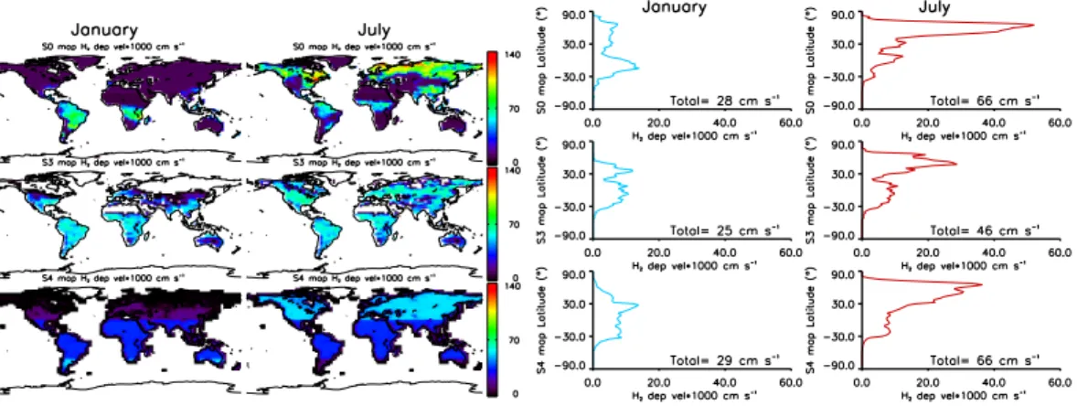
as prior in the model. These maps are presented in Fig. 4. They present some common large scale features but differ for the magnitude and distribution of regional uptake. On a large scale, the highest values are found during summer. In winter, the maximum values are located in the Southern Hemisphere and in summer they are located in the Northern Hemisphere except for the S3 map where high deposition velocities are

10

found in the Southern Hemisphere throughout the year. The first two maps (S0 and S3) are more detailed since they are based on vegetation maps. The last one (S4) was created using deposition velocity measurements. These measurements remain sparse and were thus extrapolated to latitudinal bands. The first map (S0) that supposedly underestimates the soil sink is nevertheless the one having the greatest velocities, up

15

to 0.14 cm s−1, whereas the S3 map only reaches 0.07 cm s−1 and the Oslo one (S4) only reaches 0.06 cm s−1. However, if we plot the mean latitudinal deposition velocity versus the latitude (on the lower panel), di_fferent patterns appear. S0, S3 and S4 present a similar global pattern in winter, whereas the summer total of S3 is smaller than it is in the two other maps. The yearly total reaches 42, 36 and 46 cm s−1for S0,

20

S3 and S4 respectively.

S3 is characterised by the absence of large spatiotemporal variations and the small-est global total value. In this map, there is no hotspot but a lower deposition velocity above 30◦N than below (except for the Sahara region with the desert and Australia).

S0 presents important spatiotemporal variations with marked hotspots. In the winter,

25

(16)

ACPD

10, 28963–29005, 2010

H₂ 4D-var

C. Yver et al.

Title Page

Tables Figures

◭ ◮

Back Close

Full Screen / Esc

Discussion

P

a

per

|

Dis

cussion

P

a

per

|

Discussion

P

a

per

|

Discussio

n

P

a

per

|

In S4 map, the latitudinal deposition velocity presents spatiotemporal variations as well, but contrary to S0, there are no hotspots. In winter, the larger values are found in South America and southern Africa too but more so at the southern latitudes (Argentina and South Africa). Since the soil uptake is extrapolated from latitudinal bands, there are also large values in southern Australia. In summer, the greater deposition velocities

5

are observed above 30◦N.

The three maps thereby present great differences in their distribution and we can expect to find important differences in the first-guess simulations.

4 Results and discussion

4.1 Evaluation of the first-guess and inverse simulations

10

We present, in Fig. 5, the simulated and observed mixing ratios for four sites: the north-ernmost site, Alert in Alaska, a mid-latitudinal site, Mace Head in Ireland, a northern tropical site, Pondichery in India and the southern hemispheric site, Amsterdam Island. Observations are plotted with black filled circles. Simulated mixing ratios are plotted in coloured diamonds with first-guess mixing ratios modelled with the prior emissions on

15

the left panel and inverted mixing ratios on the right panel. As S1 and S2 as well as S4 and S5 use the same prior information, their first-guess mixing ratios are superim-posed.

As previously mentioned, the first-guess mixing ratios using prior emissions from S0 are overestimated by about 115 ppb. For the other scenarios, the mixing ratios have

20

been scaled and the prior fluxes have been updated so that the mean difference is

lower than 40 ppb, except for S3, which presents a mean difference of 87 ppb due to a drift in time as the prior budget is not balanced. At Alert, the first-guess simulated seasonal cycle of S0 to S2 follows the observed cycle with a maximum in autumn and a minimum at the beginning of spring. For S3 through S5, the seasonal cycle is about

25

(17)

ACPD

10, 28963–29005, 2010

H₂ 4D-var

C. Yver et al.

Title Page

Tables Figures

◭ ◮

Back Close

Full Screen / Esc

Discussion

P

a

per

|

Dis

cussion

P

a

per

|

Discussion

P

a

per

|

Discussio

n

P

a

per

|

cycle of S0 to S2 is about two months in advance, whereas S3, S4 and S5 follow the observed cycle. For the other sites, the weak seasonal cycle is well reproduced. The first-guess mixing ratios of S3, S4 and S5 present a qualitatively better agreement with the observed seasonal cycle. The seasonal amplitude is fairly reproduced by all of the first-guess simulations except for S3, for which the seasonal amplitude is weaker.

5

For all of the sites, the first-guess mixing ratios of S3, S4 and S5 present a drift of 50, 30 and 30 ppb yr−1 respectively. This is due to the fact that the prior H₂ budget

is not balanced since we use different soil deposition maps. We also see a slight

decrease in S0 first-guess mixing ratios for Amsterdam Island which is not observed in the measurements.

10

After inversion, as expected, the simulated mixing ratios fit the observations better

in terms of amplitude as well as seasonal cycle. The mean difference between

ob-servations and simulated mixing ratios is thus nearly zero. The mean coefficient of

correlation between the observations and the simulations increases by ≈_{100%. The}

better correlation for the scenarios including the separate soil uptake optimisation is

15

found for S4 with a mean difference around −_{1.5 ppb (}₊_{35 ppb for the first-guess), a}

standard deviation of 17 ppb (47 ppb for the first-guess) and a coe_fficient of correlation of 0.6 (0.4 for the first-guess). S5, where the sources are further separated presents very close results.

4.2 Inverted fluxes

20

For each process in the H₂budget, the flux interannual variations remain small, below

±_{5 Tg yr}−1_{. All of the scenarios are consistent for the interannual variations in terms of}

pattern and amplitude (not shown). In Fig. 6, the mean seasonal cycle in 2006–2009 is plotted for all of the scenarios. For each process, we have studied three regions:

the High Northern Hemisphere (HNH) above 30◦N, the Tropics, between 30◦N and

25

30◦S and the High Southern Hemisphere (HSH) below 30◦S. As explained before,

(18)

ACPD

10, 28963–29005, 2010

H₂ 4D-var

C. Yver et al.

Title Page

Tables Figures

◭ ◮

Back Close

Full Screen / Esc

Discussion

P

a

per

|

Dis

cussion

P

a

per

|

Discussion

P

a

per

|

Discussio

n

P

a

per

|

inverted fluxes stay close to the prior fluxes. The difference of≈_{5 Tg yr}−1 _{between S0}

and the others scenarios for the photochemical production is due to the change of the prior HCHO concentrations between the first scenario and the others. The priori soil uptake and the emissions are set with a error of 100% and are therefore more subject to changes. The soil uptake seasonal cycle presents large variations in the HNH. S0

5

and S1, where the soil uptake is not separately inverted, exhibit their maximum in June. For S2, with the separated inversion of the soil uptake, the maximum is shifted in July and for S3 and S4, the maximum is shifted in August. In comparison, the soil uptake measurements, obtained with bottom-up and top-down methods and used to create the S4 deposition velocity map, are maximum at the end of August or the

10

beginning of September. Moreover, the observed mixing ratios, which are dominated by the uptake in the HNH, are minimum at the end of summer as well. The shift from June to August shows that we are able to reproduce the seasonal cycle of the soil uptake better than with the previous assumptions. In the Tropics and the Southern Hemisphere, no seasonal cycle is apparent and the mean value is consistent among

15

all of the scenarios.

In S0, it was believed that the soil sink was too weak in the HNH (Hauglustaine and Ehhalt, 2002), so in S1 and S2 we have increased this sink by 30%.

In S1, we still invert the net H2flux and the soil sink remains nearly the same as the

prior flux. In S2, since we separately invert the soil sink and the surface emissions, the

20

deposition velocities are optimised and the resulting HNH soil uptake is nearly back to the value of S0. This seems to imply that the soil uptake in S0 was not that weak but that the offset between the simulated mixing ratios and observations has other causes. Overall, the seasonal cycle of the surface emissions peaks in the HNH in June for S0 to S2 and in August for S3 to S5. This can be explained by the change in the

25

(19)

ACPD

10, 28963–29005, 2010

H₂ 4D-var

C. Yver et al.

Title Page

Tables Figures

◭ ◮

Back Close

Full Screen / Esc

Discussion

P

a

per

|

Dis

cussion

P

a

per

|

Discussion

P

a

per

|

Discussio

n

P

a

per

|

and in August/September in the north (van der Werf et al., 2006). Bousquet et al. (2010) found two peaks as well, the first one in mid-March and the second, which is also the larger one, in September. S2, S4 and S5 reproduce this same pattern. The southern maximum is clearly apparent for S1, S2 and S5 but weak for S0, S3 and S4. Except for S1, the second maximum in September is larger. We observe good

5

agreement among all of the scenarios, except for S0, for the amplitude of the summer peak. In the Southern Hemisphere, there are only very small surface emissions.

In S5, we have separately inverted the emissions in three different processes.

Biomass burning (dark green dots), anthropogenic (dark green dashes) and N2

fixation-related (dark green dashes-dots) emissions are plotted in the same panel as the total

10

surface emissions are. The prior is overplotted in light green with the same symbols for each source. The seasonality is mainly driven by the biomass burning emissions whereas the anthropogenic and N2fixation-related emissions are more or less constant

throughout the year.

From the analysis of the differences between the observations and the simulated

15

mixing ratios and from these last remarks, it can be concluded that S5 is the more pertinent scenario. Therefore, the following discussion on the H₂ budget focuses on the results of this scenario.

4.3 H₂budget

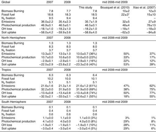
In Table 4, the mean estimation for each term of the global and regional budget is

20

calculated for 2007, 2008 and the whole period based on scenario S5. The global estimations for each term as given in Xiao et al. (2007) and Bousquet et al. (2010) are added in Table 4. The uncertainties for our study are represented by the standard deviation of scenarios S1 through S5. We do not include S0 because, in this scenario, the prior HCHO flux is≈_{5 Tg yr}−1 _{lower than the prior flux in the other scenarios and,}

25

(20)

ACPD

10, 28963–29005, 2010

H₂ 4D-var

C. Yver et al.

Title Page

Tables Figures

◭ ◮

Back Close

Full Screen / Esc

Discussion

P

a

per

|

Dis

cussion

P

a

per

|

Discussion

P

a

per

|

Discussio

n

P

a

per

|

standard deviation of the sensitivity inversions based on the reference scenario (ex-ternal errors). The errors in Xiao et al. (2007) include model uncertainties, absolute calibration error and errors in the assumed transportation source strength. For each region, we indicate the relative proportion of each regional source or sink in compari-son with the global source or sink. Figure 7 represents this budget per process and per

5

region. All of the scenarios produce a consistent process-based view (maximum stan-dard deviation of 15%). From a region-based view, the total H2flux ranges between−8

and+8 Tg yr−1. For these small fluxes, it is not adequate to use the relative standard deviation (varying between 18% and 160%) but we observe standard deviations below 2 Tg yr−1. For all of the scenarios, the HNH is a net sink of H2 and the Tropics are a

10

net source. Globally,≈_{47 Tg yr}−1_{of H}₂_{are produced by photochemical production and} ≈_{18 Tg yr}−1 _{are consumed by the OH reaction. Approximately 36 Tg yr}−1_{are emitted}

and ≈_{59 Tg yr}−1 _{are deposited in the soils. This budget leads to a tropospheric}

bur-den of 166 Tg and a life time of 2.2 years. This budget is consistent with most of the previous studies about H₂cycle.

15

Every process has a larger flux in the Tropics than it has in the HNH or HSH. Tropical processes represent between 55% and 74% of global processes depending on the flux types. Indeed, the photochemical production and the OH sink depend strongly on insolation which is maximum in the Tropics. The tropical maximum in the surface emissions is due to biomass burning emissions. For the maximum of soil uptake in the

20

Tropics (55%), as Xiao et al. (2007) have already proposed, one explanation could be that the tropical soils are more efficient in terms of uptake than the extra-tropical soils are. It could also be linked to the optimum conditions in the humidity and temperature of this region. The soil sink in the HNH nevertheless represents 40% of the global soil sink.

25

(21)

ACPD

10, 28963–29005, 2010

H₂ 4D-var

C. Yver et al.

Title Page

Tables Figures

◭ ◮

Back Close

Full Screen / Esc

Discussion

P

a

per

|

Dis

cussion

P

a

per

|

Discussion

P

a

per

|

Discussio

n

P

a

per

|

work. The repartition between the different regions is more consistent with Xiao et al. (2007) than with Bousquet et al. (2010). This result can be explained by the fact that, in this study and in Xiao et al. (2007), the budget was analysed through the same lat-itudinal bands, whereas Bousquet et al. (2010) used large regions that did not exactly fit these latitudinal bands. Finally, our estimate of biomass burning-related emissions

5

is the same order of magnitude as Bousquet et al. (2010) and Xiao et al. (2007) but our estimation represents only 22% of the total emissions against 31% and 44% for Bousquet et al. (2010) and Xiao et al. (2007), respectively.

4.4 Focus on Europe

In this study, Europe contains the largest number of observation sites. Therefore, one

10

can expect to have sufficient constraints to improve our knowledge on the sources and sinks of H₂ for this part of the world. As seen in Fig. 7, Europe, as part of the HNH, seems to be a net sink of H2. In Fig. 8, the posterior flux map and the difference

be-tween posterior and prior in percentage of the prior for the S5 surface emissions and soil uptake are plotted. To observe the di_fference better, the data are interpolated on

15

a higher resolution grid (1◦×₁◦_{). The emissions in Europe present the same pattern}

in the spring and autumn. However, in the autumn, the emissions are slightly higher (maximum of 8 Tg yr−1), than they are in the spring (maximum of 5 Tg yr−1). This au-tumnal flux can be explained, from the seasonal cycle (see Fig. 6), by a combination of enhanced biomass burning and N2fixation-related emissions at the end of the

sum-20

mer and a small increase of the anthropogenic emissions at the end of the year. The differences between prior and posterior range from−_{60 to 0% in spring and from}−₁₅

to +30% in autumn for the emissions. This means that in spring, the inversion

re-duces European prior emissions, especially in western Europe. In autumn, western prior emissions are only slightly decreased, but eastern prior emissions are largely

in-25

(22)

ACPD

10, 28963–29005, 2010

H₂ 4D-var

C. Yver et al.

Title Page

Tables Figures

◭ ◮

Back Close

Full Screen / Esc

Discussion

P

a

per

|

Dis

cussion

P

a

per

|

Discussion

P

a

per

|

Discussio

n

P

a

per

|

the alpine region in autumn. The differences between prior and posterior range from

−_{7 to} ₊_{35% in spring and from} −_{58 to} ₊_{10% in autumn. The spring soil uptake is}

increased in all of Europe compared to the prior estimate. In autumn, a large decrease of the prior soil uptake is found for northern Europe, whereas western Europe flux is increased compared to the prior.

5

In Table 5, the emissions and the soil uptake are detailed for seven countries or groups of countries in Table 5: geographical Europe (including the European part of Russia, west of the Ural mountains); Europe (27 countries); France; Germany; the United Kingdom and Ireland; Scandinavia and Finland; Spain, Italy and Portugal. In terms of emissions, geographical Europe represents 6% and 18% of the global and

10

HNH emissions respectively. The European soil uptake accounts for 7% and 17% of the global and HNH uptake respectively. Anthropogenic emissions account for 52% of the total emissions globally, 62% in the HNH and 72% in Europe (27 countries). In Europe, depending on the countries, anthropogenic emissions account for 50% to 100% of the total emissions. As written above, there is no bottom-up inventory of H2

15

emissions. We have then compared our results with the inventory from the Institute for Energy and Environmental Research (IEER) (Thiruchittampalam and K ¨oble, 2004), which is not used as prior information (see Table 5). We have scaled the CO emis-sions with the anthropogenic H2/CO mass ratio of 0.034 as found in Yver et al. (2009).

The two sets of values agree well with one another. The mean difference lies around

20

10%. Uncertainties on inventories are not yet produced quantitatively but the EDGAR

database has proposed ranges of uncertainties: low (±_{10%), medium (}±_{50%) and}

large (±_{100%) (Olivier et al., 1996). For CO, most uncertainties by source types are}

reported as “medium”, therefore making our results consistent with IEER estimates, within their respective uncertainties.

(23)

ACPD

10, 28963–29005, 2010

H₂ 4D-var

C. Yver et al.

Title Page

Tables Figures

◭ ◮

Back Close

Full Screen / Esc

Discussion

P

a

per

|

Dis

cussion

P

a

per

|

Discussion

P

a

per

|

Discussio

n

P

a

per

|

5 Conclusions

This work presents the results of an inversion of tropospheric H2 sources and sinks

at a grid cell resolution for the period between mid-2006 and mid-2009. The model focuses on soil uptake and surface emissions. Overall, the results of this study agree with those of previous studies with regard to a lifetime of about two years, a soil uptake

5

of≈_{58 Tg yr}−1_{and emissions of}≈_{34 Tg yr}−1_{for a total source of}≈_{80 Tg yr}−1_{. All of the}

inversions performed with the six scenarios are fairly consistent with one another in terms of the processes (standard deviation≈_{15%) and the regions (standard deviation}

<_{2 Tg yr}−1_{). From the several scenarios that have been elaborated, the best one (S5)}

in terms of fit to the mean atmospheric mixing ratio, seasonal cycle and flux

measure-10

ments combines a separate inversion of the soil sink and of the sources in three terms and a soil deposition velocity map based on soil uptake measurements. Our estima-tion for the global soil uptake is−₅₉±_{4 Tg yr}−1_{. Ninety-five per cent of this uptake is}

located in the HNH (40%) and the Tropics (55%). No significant trend is found for the soil uptake or any of the other processes of the H2budget throughout 2006–2009. To

15

study the emissions better, one scenario (S5), has been implemented with a separate inversion of the sources in three processes (biomass burning, fossil fuel and N2fixation

related emissions). This scenario shows that the seasonal variability of the emissions is mainly driven by the biomass burning emissions. Finally, we have focused our analy-sis on Europe and compared the anthropogenic emissions with a CO inventory scaled

20

with a H2/CO mass ratio of 0.034. Anthropogenic emissions represent 50% to 100% of

the total emissions depending on the country. The model and the inventory agree with one another within their respective uncertainties. A further step will be to invert other relevant species with H2such as CH4, CO and HCHO, which is a unique capability of

our multispecies inversion system (Pison et al., 2009). In particular, the optimisation of

25

(24)

ACPD

10, 28963–29005, 2010

H₂ 4D-var

C. Yver et al.

Title Page

Tables Figures

◭ ◮

Back Close

Full Screen / Esc

Discussion

P

a

per

|

Dis

cussion

P

a

per

|

Discussion

P

a

per

|

Discussio

n

P

a

per

|

Future inversions of H2 sources and sinks should gain robustness by including

ob-servations of other networks but also by including obob-servations of the deuterium en-richment of H2(δDof H2), as shown in Rhee et al. (2006); Price et al. (2007). Several

groups have produced δD _{observations (Gerst and Quay, 2001; Rahn et al., 2003;}

R ¨ockmann et al., 2003; Rhee et al., 2006; Price et al., 2007). Within the

EUROHY-5

DROS project, δD _{observations from six sampling sites are available for the recent}

years (from 2006). The isotopic signatures for fossil fuel, biofuel, biomass burning,

and ocean sources are all depleted inδD relative to the atmosphere, whereas

pho-tochemical production of H2 has a large positive isotopic signature. On the sink side,

OH loss fractionates more than soil uptake (Price et al., 2007). The troposphericδD

10

is about₊130±_{4% (Gerst and Quay, 2000). Assimilating}δD observations together

with H2 observations could bring new constraints on H2budget if the different isotopic

signatures can be determined with a good precision.

Acknowledgements. We gratefully thank Mathilde Grand and Vincent Bazantay for performing the flasks and in-situ analyses for the RAMCES network as well as the people involved in the

15

samplings and analyses for the EUROHYDROS network. Thank you to Fr ´ed ´eric Chevallier for the precious help on the modelling part and to the computing support team of the LSCE. This work was carried out under the auspices of the 6th EU framework program # FP6-2005-Global-4 “EUROHYDROS- A European Network for Atmospheric Hydrogen Observations and Studies”. RAMCES is funded by INSU and CEA.

20

(25)

ACPD

10, 28963–29005, 2010

H₂ 4D-var

C. Yver et al.

Title Page

Tables Figures

◭ ◮

Back Close

Full Screen / Esc

Discussion

P

a

per

|

Dis

cussion

P

a

per

|

Discussion

P

a

per

|

Discussio

n

P

a

per

|

References

Aalto, T., Lallo, M., Hatakka, J., and Laurila, T.: Atmospheric hydrogen variations and tra_ffic emissions at an urban site in Finland, Atmos. Chem. Phys., 9, 7387–7396, doi:10.5194/acp-9-7387-2009, 2009. 28970

Bonasoni, P., Calzolari, F., Colombo, T., Corazza, E., Santaguida, R., and Tesi, G.: Continuous

5

CO and H₂measurements at Mt. Cimone (Italy): Preliminary results, Atmos. Environ., 31, 959–967, 1997. 28970

Bond, S., Vollmer, M., Steinbacher, M., Henne, S., and Reimann, S.: Atmospheric molecular hydrogen (H₂): Observations at the high-altitude site Jungfraujoch, Switzerland, Tellus B, doi:10.1111/j.1600-0889.20100059.x, 2010. 28970

10

Bousquet, P., Hauglustaine, D. A., Peylin, P., Carouge, C., and Ciais, P.: Two decades of OH variability as inferred by an inversion of atmospheric transport and chemistry of methyl chlo-roform, Atmos. Chem. Phys., 5, 2635–2656, doi:10.5194/acp-5-2635-2005, 2005. 28973, 28974

Bousquet, P., Yver, C., Pison, I., Li, Y. S., Fortems, A., Hauglustaine, D., Szopa, S., Peylin, P.,

15

Novelli, P., Langenfelds, R., Steele, P., Ramonet, M., Schmidt, M., Simmonds, P. G., Foster, P., Morfopoulos, C., and Ciais, P.: A 3-D inversion of the global hydrogen cycle: implications for the soil uptake flux, J. Geophys. Res., accepted, 2010. 28968, 28976, 28981, 28982, 28983, 28996

Brasseur, G. P., Hauglustaine, D. A., Walters, S., Rasch, P. J., M ¨uller, J., Granier, C., and Tie,

20

X. X.: MOZART, a global chemical transport model for ozone and related chemical tracers 1. Model description, J. Geophys. Res., 103, 28265–28290, 1998. 28975

Carouge, C., Bousquet, P., Peylin, P., Rayner, P. J., and Ciais, P.: What can we learn from European continuous atmospheric CO₂ measurements to quantify regional fluxes – Part 1: Potential of the 2001 network, Atmos. Chem. Phys., 10, 3107–3117,

doi:10.5194/acp-10-25

3107-2010, 2010. 28974

Chevallier, F., Fisher, M., Peylin, P., Serrar, S., Bousquet, P., Br ´eon, F., Ch ´edin, A., and Ciais, P.: Inferring CO2 sources and sinks from satellite observations: Method and application to TOVS data, J. Geophys. Res., 110, D24309, doi:10.1029/2005JD006390, 2005. 28972, 28974

30

(26)

ACPD

10, 28963–29005, 2010

H₂ 4D-var

C. Yver et al.

Title Page

Tables Figures

◭ ◮

Back Close

Full Screen / Esc

Discussion

P

a

per

|

Dis

cussion

P

a

per

|

Discussion

P

a

per

|

Discussio

n

P

a

per

|

Conrad, R. and Seiler, W.: Influence of temperature, moisture, and organic carbon on the flux of H₂and CO between soil and atmosphere: Field studies in subtropical regions, J. Geophys. Res., 90, 5699–5709, 1985. 28966

Ehhalt, F. R. D. H.: The tropospheric cycle of H₂: A critical review, Tellus B, 61, 500–535, 2009. 28966, 28967

5

Engel, A.: EUROHYDROS, A European Network for Atmospheric Hydrogen observa-tions and studies., in: EUROHYDROS Final Report, http://cordis.europa.eu/fetch? CALLER=FP6 PROJ&ACTION=D&DOC=1&CAT=PROJ&QUERY=012bab525b95:d528: 5b2afd2e&RCN=80080, 2009. 28967, 28970, 28971

Erickson, D. J. and Taylor, J. A.: 3-D tropospheric CO modeling - The possible influence of the

10

ocean, Geophys. Res. Lett., 19, 1955–1958, 1992. 28975

Gerst, S. and Quay, P.: The deuterium content of atmospheric molecular hydrogen: Method and initial measurements, J. Geophys. Res., 105, 26433–26446, 2000. 28986

Gerst, S. and Quay, P.: Deuterium component of the global molecular hydrogen cycle, J. Geo-phys. Res., 106, 5021–5029, 2001. 28986

15

Granier, C., Hao, W. M., Brasseur, G., and M ¨uller, J.-F.: Land use practices and biomass burning: Impact on the chemical composition of the atmosphere, in Biomass Burning and Global Change, edited by: Levine, J. S., MIT Press, Cambridge, Mass., 1996. 28975 Grant, A., Witham, C. S., Simmonds, P. G., Manning, A. J., and O’Doherty, S.: A 15 year record

of high-frequency, in situ measurements of hydrogen at Mace Head, Ireland, Atmos. Chem.

20

Phys., 10, 1203–1214, doi:10.5194/acp-10-1203-2010, 2010b. 28966, 28970

Hammer, S. and Levin, I.: Seasonal variation of the molecular hydrogen uptake by soils inferred from continuous atmospheric observations in Heidelberg, southwest Germany, Tellus, 61B, 556–565, 2009. 28969, 28970

Hammer, S., Vogel, F., Kaul, M., and Levin, I.: The H₂/CO ratio of emissions from combustion

25

sources: comparison of top-down with bottom-up measurements in southwest Germany, Tellus, 61B, 547–555, 2009. 28970

Hao, W. M., Ward, D. E., Olbu, G., and Baker, S. P.: Emissions of CO₂, CO, and hydrocarbons from fires in diverse African savanna ecosystems, J. Geophys. Res., 101, 23577–23584, 1996. 28975

30

(27)

ACPD

10, 28963–29005, 2010

H₂ 4D-var

C. Yver et al.

Title Page

Tables Figures

◭ ◮

Back Close

Full Screen / Esc

Discussion

P

a

per

|

Dis

cussion

P

a

per

|

Discussion

P

a

per

|

Discussio

n

P

a

per

|

Hauglustaine, D. A., Hourdin, F., Jourdain, L., Filiberti, M. A., Walters, S., Lamarque, J. F., and Holland, E. A.: Interactive chemistry in the Laboratoire de Meteorologie Dynamique general circulation model: Description and background tropospheric chemistry evaluation, J. Geophys. Res., 109, D04314, doi/10.1029/2003JD003957, 2004. 28973

Hough, A. M.: Development of a Two-Dimensional Global Tropospheric Model: Model

Chem-5

istry, J. Geophys. Res., 96, 7325–7362, 1991. 28975

Hourdin, F. and Armengaud, A.: The Use of Finite-Volume Methods for Atmospheric Advection of Trace Species. Part I: Test of Various Formulations in a General Circulation Model, Mon. Weather Rev., 127, 822–837, 1999. 28972

Hourdin, F. and Talagrand, O.: Eulerian backtracking of atmospheric tracers. I: Adjoint

deriva-10

tion and parametrization of subgrid-scale transport, Q. J. Roy. Meteorol. Soc., 132, 567–583, 2006. 28972

Jordan, A.: The EUROHYDROS calibration scale for hydrogen, 14th WMO/IAEA Meeting of Experts on Carbon Dioxide, Other Greenhouse Gases, and Related Tracer Measurement Techniques, 2007. 28970

15

Jordan, A. and Steinberg, B.: Calibration of atmospheric hydrogen measurements, Atmos. Meas. Tech. Discuss., 3, 4931–4966, doi:10.5194/amtd-3-4931-2010, 2010. 28970

Khalil, M. A. K. and Rasmussen, R. A.: Global increase of atmospheric molecular hydrogen, Nature, 347, 743–745, 1990. 28966

Krol, M. C., Lelieveld, J., Oram, D. E., Sturrock, G. A., Penkett, S. A., Brenninkmeijer, C. A. M.,

20

Gros, V., Williams, J., and Scheeren, H. A.: Continuing emissions of methyl chloroform from Europe, Nature, 421, 131–135, 2003. 28973, 28974

Lallo, M., Aalto, T., Laurila, T., and Hatakka, J.: Seasonal variations in hydrogen de-position to boreal forest soil in southern Finland, Geophys. Res. Lett., 35, L04402, doi:10.1029/2007GL032357, 2008. 28966, 28969

25

Lallo, M., Aalto, T., Hatakka, J., and Laurila, T.: Hydrogen soil deposition at an urban site in Finland, Atmos. Chem. Phys., 9, 8559–8571, doi:10.5194/acp-9-8559-2009, 2009. 28966, 28969

Lamarque, J.-F., Granier, C., Bond, T., Eyring, V., Heil, A., Kainuma, M., Lee, D., Liousse, C., Mieville, A., Riahi, K., Schultz, M., Smith, S., Stehfest, E., Stevenson, D., Thomson, A.,

30

Aardenne, J. V., and Vuuren, D. V.: Gridded emissions in support of IPCC AR5, IPCC, 34, 2008. 28975, 28976