Adjusting to external imbalances within the EMU, the case of Portugal

(1)

Adjusting to external imbalances within the

EMU, the case of Portugal

Francesco Franco

∗

27-4-2011 (First version 10-2010)

The Portuguese economy is in serious trouble: Productivity

growth is anemic. Growth is very low. The budget deficit is large.

The current account deficit is very large.

Olivier Blanchard (2007)

Abstract

From 1995 to 2010 Portugal has accumulated a negative

interna-tional asset position of 110 percent of GDP. In a developed and aging

economy the number is astonishing and any argument to consider it

sustainable must rely on extremely favorable forecasts on growth.

Por-tuguese policy options are reduced in number: no autonomous

mone-tary policy, no currency to devaluate, and limited discretion in

chang-∗_{Faculdade de Economia, Universidade Nova de Lisboa. Contact: [email protected]. I}

(2)

ing fiscal deficits and government debt. To start the necessary

delever-aging a remaining possible policy is a budget-neutral change of the tax

structure that increases private saving and net exports. An increase in

the VAT and a decrease in the employer’s social security contribution

tax can achieve the desired outcome in the short run if they are

comple-mented with wage moderation. To obtain a substantial improvement

in competitiveness and a large decrease in consumption, the changes

in the tax rates have to be large. While a precise quantitative

assess-ment is difficult, the initial increase in the effective VAT rate needed to

allow the social security tax to decrease by 16 percentage points (pp)

is approximately 10 pp. Such a large increase in the effective VAT rate

could be obtained by raising most of the reduced VAT rates to the new

general VAT rate of 23 percent. The empirical analysis shows that over

time the suggested tax swap could generate surpluses and improve the

trade balance. A temporary version of the suggested tax-swap has

the attractiveness to achieve a sharper increase in the private saving

rate maintaining the short run gains in competitiveness. Finally, the

temporary version of the fiscal devaluation could be the basis for an

(3)

-1.5

-1.5 -1

-1

-1 -.5

-.5

-.5 0

0

0 1995q1

1995q1 1995q1 2000q1

2000q1 2000q1

2005q1

2005q1 2005q1

2010q1

2010q1 2010q1

Accumulated current account

Accumulated current account Accumulated current account

NIIP

NIIP NIIP

The data are shown as a percentage of GDP.Sources:Banco de Portugal and Eurostat

The data are shown as a percentage of GDP.Sources:Banco de Portugal and Eurostat The data are shown as a percentage of GDP.Sources:Banco de Portugal and Eurostat

Net External Position

Figure 1: Net International Investment Position

Portugal has been running large current account deficits every year since

1995. These deficits have accumulated to an astonishing 110 percent of GDP

negative external asset position.

The sustainability of such a large external position is questionable and

must rely on fantastic productivity growth expectations. The recent global

financial crisis appears to have anticipated the international investors

real-ity check on those future expectations with the result of a large increase in

the cost of external financing. Today the rebalancing of the current account

through an increase in national savings and an improvement in

competitive-ness must be at the top of the Portuguese authorities “to do” list as the cost

(4)

external rebalancing is difficult as the degrees of freedom of the Portuguese

authorities are limited in number: they have no autonomous monetary

pol-icy, no currency to devaluate, and little discretion in fiscal policy as deficit

limits and debt targets are set by the Stability Growth Pact and the

post-crisis consensus on medium-term fiscal consolidation. One possibility that

remains is to change the fiscal policy mix for a given budget deficit. The

purpose of this paper is to explore the effects of a “fiscal devaluation”1

ob-tained through a tax swap between employers’ social security contributions

and taxes on consumption2

. The paper begins by illustrating Portugal’s

cur-rent account evolution during the euro period. The second section section

lays out a model to offer a qualitative assessment of the dynamic outcomes of

the the tax swap. I show that the suggested tax swap can in theory achieve

the desired outcomes in terms of competitiveness and consumption if

com-plemented with moderation (stickiness) in wages. I also study the effects of

a temporary version of the tax swap and show that it achieves a sharper

im-provement in the current account that accelerate the rebalancing. The third

section moves to the empirical analysis and estimates the likely effects of the

tax swap for the Portuguese economy. The fourth section concludes.

1

See Domingo and Cottani (2010) for a recent proposal of fiscal devaluation in Portugal, Greece and Spain.

2

(5)

.62 .6 2 .62 .64 .6 4 .64 .66 .6 6 .66 .68 .6 8 .68 Private consumption P ri v a te c on s u mp ti on Private consumption 2000 2000 2000 2002 2002 2002 2004 2004 2004 2006 2006 2006 2008 2008 2008 2010 2010 2010 date date date .18 .1 8 .18 .2 .2 .2 .22 .2 2 .22 .24 .2 4 .24 .26 .2 6 .26 .28 .2 8 .28 Private investment P ri v a te i n v e s tme n t Private investment 2000 2000 2000 2002 2002 2002 2004 2004 2004 2006 2006 2006 2008 2008 2008 2010 2010 2010 date date date -.14 -.14 -.14 -.12 -.12 -.12 -.1 -.1 -.1 -.08 -.08 -.08 -.06 -.06 -.06

Current Account & Net Exports

C u rr e n t A c c ou n t & N e t E x p or ts

Current Account & Net Exports 2000 2000 2000 2002 2002 2002 2004 2004 2004 2006 2006 2006 2008 2008 2008 2010 2010 2010 date date date CA CA CA TB TB TB .19 .1 9 .19 .2 .2 .2 .21 .2 1 .21 .22 .2 2 .22 Government consumption G ov e rn me n t c on s u mp ti on Government consumption 2000 2000 2000 2002 2002 2002 2004 2004 2004 2006 2006 2006 2008 2008 2008 2010 2010 2010 date date date

The data are shown as a percentage of GDP. Source:Eurostat

The data are shown as a percentage of GDP. Source:Eurostat The data are shown as a percentage of GDP. Source:Eurostat

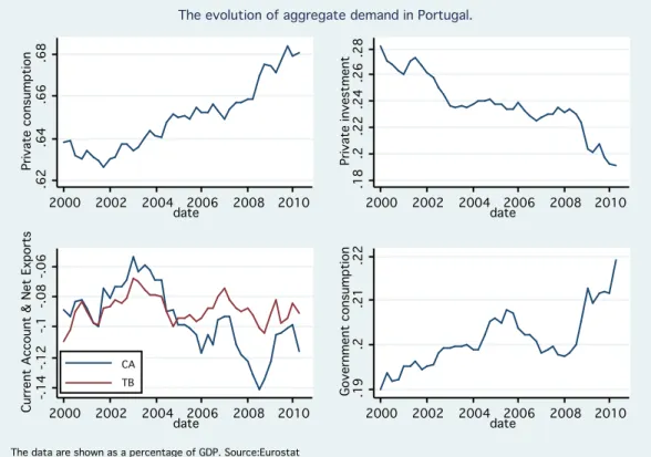
The evolution of aggregate demand in Portugal.

Figure 2: Aggregate demand in Portugal

Portugal in the Euro

Figure 2 shows the evolution of Portugal’s aggregate demand since the launch

of the Euro.

In words, it shows that private consumption as a share of GDP increased

from 63 to 68 percent, private investment decreased from 28 to 19 percent, net

exports oscillated around -9 percent and Government consumption went from

19 to 22 percent. The latter declined from 2005-6 but then started to increase

again in 2008. The accumulated deficit of the last 15 years is reflected in the

large negative net external position3

shown in Figure 1, which, according

3

(6)

to the IMF, reached the all time record of 113 percent of GDP in 2009. A

lucid and prescient account on the Portuguese economy evolution is given by

Blanchard (2007), from which I took the introductory citation, and can be

synthesized as follows:

• from 1995 to 2001 (not shown) the participation in the ERM and the buildup of the euro caused a nominal convergence (inflation, interest

rates, country risk not decoupling from currency risk) coupled with

expectations of real convergence (productivity). The result was an

increase in both consumption and investment. The expectations of

real convergence justified a benign interpretation of the current account

deficit increase.

• from 2001 to 2007 real convergence did not occur and the boom turned into a bust. The current account continued to increase as the real

ex-change rate appreciated and competitiveness plummeted. The reality

check on real convergence expectations shifted the interpretation of the

current account deficits from benign to malign but Euro membership

shielded Portugal from a refusal to finance additional increases in debt

as the spreads with the core euro zone countries were almost

nonexis-tent.

An intuitive reading of Figure 2 suggests thatPortugal must increase private

saving by decreasing consumption and improve its net exports. It is worth

noting that the statements on saving and net exports are conditional on

(7)

the hypothesis that Portugal current external position is not following an

equilibrium path. To see this more formally consider the following thought

experiment. First describe the process that brought Portugal to its current

state with a non identified and unexpected reduced form aggregate shock.

Second compute the equilibrium responses of a canonical small-open economy

that belongs to a monetary union. For simplicity I assume that the long-run

equilibrium (steady state) of the economy has a balanced current account and

net foreign asset position but suddenly (shock) founds itself with a negative

NIIP of 110 percent of GDP and a current account deficit of 10 percent of

(8)

(9)

Figure 3 shows that after such a shock the economy response is to

re-duce consumption and increase saving. The decrease in demand deflates the

economy which in turn increases competitiveness and allow to run a positive

trade balance. Net foreign debt is repaid in time with the generated trade

balance surpluses. In reality, there was no such shock but a lengthy process,

illustrated in Figure 2, that brought the economy to the current position, and

in particular this process has been characterized by the absence of the

theo-retical adjustment (equilibrium responses) illustrated in Figure 3. This last

observation suggests that the “self equilibrating” forces in the economy are

at best slow in Portugal and that a policy that accelerates or even initiates

the required adjustment is necessary. In the pre-EMU era, the natural policy

to help the adjustment was to devalue the currency. Today Portugal must

find policies that permit a “synthetic” devaluation. In the current limited

policy option framework, this could be achieved with a decrease in wages

and/or a tax swap from employers’ contributions to social security to VAT.

The former solution is politically difficult and possibly unconstitutional in

Portugal. The latter can achieve an increase in saving by reducing the

at-tractiveness of consumption and an increase in competitiveness by decreasing

labor costs. I now turn to the description of the model underlying Figure 3

and the implementation of a fiscal devaluation within that model.

A framework

The traditional objective of a currency devaluation is to achieve an

(10)

in this way, stimulate the economy. A fiscal devaluation corresponds to a

change in the fiscal structure of a country without its own currency aimed at

achieving similar4

objectives. Several authors have studied different aspects

of the question. The classical paper on the effects of a VAT on

competitive-ness for a small price-taking neoclassical economy is Feldstein and Krugman

(1989). These authors find that “the substitution of value-added taxation for

income taxation is likely to have an uncertain short-run effect on a nation’s

net exports but is likely to reduce net exports in the longer term”. In their

framework, the decrease in the income tax has a substitution effect that

fa-vors saving, and therefore the trade balance, in the first period. However

when VAT is selective and fall more heavily on traded goods, it will

dis-tort demand towards nontradables pulling out resources from the tradable

sector and decreasing net exports in the second period. A more recent and

closely related study, is a ECB working paper by Lipinska and Von Thadden

(2009). These authors use a two-country monetary union DSGE model to

study unilateral shifts that direct the tax structure more strongly toward

in-direct taxes5

. They find that the effects following such a shift are very small.

Implicitly many recent papers that contain open economy models with taxes

are related to this work. Most of these works introduce into an economy

that is neoclassical in nature in the long-run, some new-Keynesian feature

in the short run. The choice of which feature to introduce in the model

4

The aim of this paper is purely applied, namely to study alternative policy to nominal devaluation to improve Portugal external position. Recently Adino, Correia and Teles (2009) perform the more theoretically oriented exercise to find a set of tax instruments that allow to replicate the allocation achieved by a nominal devaluation.

5

(11)

obviously has important consequences. For example, the cited Lipinska and

Von Thadden (2009) which explicitly study the effects of a fiscal devaluation

though a tax swap between VAT and labor income taxes use a model with

price rigidities but competitive labor markets with flexible wages. Below I

show that the flexible nominal wage assumption has important consequence

as it neutralizes the demand side effects for the fiscal devaluation. In other

words with flexible nominal wage the effects of a fiscal devaluation are purely

neoclassical in nature. To organize thoughts I present in the next section a

canonical New Keynesian small open economy used to obtain Figure 3. I

have left the detailed microfounded description of the economy to an

ap-pendix and show a convenient and more intuitive log-linear approximation of

the model. Finally I present the model’s features in sequential steps to better

identify the role of each assumption discuss their plausibility in describing

the Portuguese reality.

A benchmark

Households consume and supply labor. Given that the objective is to

un-derstand the effects of a fiscal devaluation on competitiveness I start by

describing the labor-production side of the economy. In their role of

work-ers, households have some monopoly power (maybe through a union), which

allows them to set the wage, wt, for the labor services they supply, as a

mark-up µw over their marginal rate of substitutionmrst

6

(12)

mrst=

1

σct+φnt+τc,t (1)

where ct is consumption, nt is labour, τc,t is the effective consumption tax,

σ is the intertemporal elasticity of substitution and φ is the labor supply

elasticity. Domestic firms produce using only labor and have market power

in the goods market which allows them to set the price of the good they

produce, pH, as a mark-up,µp, over their marginal cost, mct

7

mct=τw,t+wt+

a

1−ayt−log(1−a) (2)

where τw,t is the social security contribution tax rate, yt is output and

a ∈ [0,1] parametrizes the degree of decreasing returns in labor. These

two equations are key to the fiscal devaluation. Consider a decrease in the

social security contributions tax rate∆τw,t<0, where∆is the first difference

operator. Other things equal, the marginal cost of the firm decreases, which

allows the firm to lower its price. This is the channel through which the

fis-cal devaluation improves competitiveness. Second consider an increase in the

consumption tax∆τc,t>0. Other things equal, the marginal rate of

substitu-tion increases pushing the worker/union to ask for a higher wage. Combining

the two changes in taxes it is immediate to see that if∆τc,t =−∆τw,t,call it a

proportional tax swap, the lower taxes effect on the marginal cost is exactly

offset by the increase in the nominal wage, leaving the initial price set by

the firm unchanged. In terms of competitiveness, when prices and wages are

7

I present the economy average marginal cost of substitution to keep the exposition simple. Formally (see the Appendix) each firm sets its own price pH₍_i₎ _{over its own}

(13)

flexible, this proportional tax swap is neutral on unit labor costs and only

increases the real wage.

Firms are assumed to adjust their prices following a model due to Calvo

(1983) characterized by random price durations which leads to a New

Key-nesian Phillips Curve for domestic price inflation

πH_t =βEtπtH+1+κ

p_mc

t (3)

whereβis the discount factor andκp _{the elasticity of domestic inflation to}

the marginal cost. Nominal price rigidity does not alter the neutral outcome

of the proportional tax swap: as marginal costs did not change, there is no

incentive for firms to change prices so that any impediment to price

adjust-ment is irrelevant. Workers also face Calvo-type constraints on the frequency

with which they can adjust wages and this leads to a New Keynesian Phillips

Curve for domestic wage inflation

πWt =βEtπWt+1+κw(mrst−wt) (4)

whereπWt is wage inflation andκwthe elasticity of domestic wage inflation

to the gap between the marginal rate of substitution and the nominal wage.

Now wage setters want to ask a higher nominal wage after the increase in

τc,t, but nominal wage rigidity implies that nominal wage will fully reflect the

increase in the marginal rate of substitution only after a period of adjustment.

During the time when nominal wages adjust to their higher level, the decrease

in the social security contribution decreases the marginal cost of the firm

(14)

irrelevant while nominal wage rigidity is necessary for the proportional tax

swap to affect competitiveness.

The intertemporal consumption-saving decision is described by a standard

intertemporal condition

ct=Etct+1−σ(it−Et[πt+1+ ∆τc,t+1]−ρ) (5)

where it is the one period run nominal interest rate, πt is the CPI rate

of inflation (net of VAT taxes), and Et is the mathematical expectation

conditional on information at time t. The relevant CPI inflation rate is given

by

πt =πtH +α∆st (6)

where πH

t =pHt −pHt−1 is the domestic goods inflation, st ≡ pF

t

pH

t is the terms of trade (ratio of the foreign goods price index over the domestic goods price

index) andα ∈[0,1]is the weight of foreign goods in domestic consumption.

The international asset market is restricted to a one-period nominal bond

with a debt-elastic interest-rate premium on the rest of the union interest

rate8

it=i ∗

t +ρ(bt) (7)

wherei∗

t is the EMU one period nominal interest rate andρ(bt)is the

do-mestic risk premium that depends on the level in real terms of the net external

8

(15)

position bt. A permanent tax swap does not affect the saving-consumption

decision given that ∆τc,t+1 = 0 in equation 5. However an expected

tran-sitory increase in the consumption tax creates an expected negative step in

the relevant interest rateit−Et[πt+1+ ∆τc,t+1]for the household

intertempo-ral decisions, increasing the attractiveness of future (post tax swap reversal)

consumption relative to current consumption.

The equilibrium in the goods market requires

yt=χst+χFst+ζct+ζFc ∗

t (8)

wherec∗

t is the EMU consumption,χis the elasticity of domestic demand

to the terms of trade, χF _{is the elasticity of exports to the terms of trade,}

ζ is the elasticity of output to domestic demand and ζF _{is the elasticity of}

output to foreign demand.

Fiscal devaluation as a proportional tax swap

I have described a fiscal devaluation as a proportional tax swap, namely a

precise change in the two tax rates such that ∆τc,t = −∆τw,t, and argued

that when such a swap is permanent the final outcome of the policy is neutral

on allocations and only results in a higher real wage. This neutrality is

ob-viously a particular case but is appealing as it permits to compare the fiscal

devaluation to a classical nominal devaluation which is also neutral on

allo-cations in the long run. In other words, in the model above, the proportional

tax swap only affects the allocations through demand channels, just like a

(16)

allocations through well understood neoclassical supply channels, which in

the case of the suggested tax swap tend to offset each other. I choose to

maintain the proportional tax swap as a benchmark for the fiscal

devalua-tion as demand forces should be more relevant in the short run, the frequency

of interest of this work. A nominal devaluation is also usually implemented

to reduce unit labour costs relative to foreign competitors, expand exports

and reduce imports, i.e. to increase in competitiveness9

. Both devaluations

can only achieve those objectives if the switching-expenditure towards

do-mestic goods is strong enough. In the benchmark model the latter requires

the elasticity of substitution between domestic and foreign goods to be large

enough. In the model net exports in terms of consumption, nxt, are

nxt =shx((λ−1)st+c ∗

t)−shm((1−λ)qt+ct) (9)

where λ is the elasticity of substitution between foreign and domestic

goods, qt ≡ P∗

t

Pt is the real exchange rate, shx is the share of exports in the trade balance and shm is the share of imports in the trade balance. To

recapitulate the proportional tax swap, when nominal wages are sticky,

im-proves external competitiveness by allowing producers to lower their prices,

increases foreign demand and can provoke an expenditure switching towards

domestic goods that lowers imports if the elasticity of substitution between

foreign and domestic goods is sufficiently large and the increase in domestic

9

(17)

demand is sufficiently low. The last two qualifications might appear

restric-tive but they are essentially the same restrictions for a nominal devaluation

having a positive effect on the trade balance. Finally, an important aspect

is the duration of the tax swap. A permanent tax swap, only affects the

competitiveness of the economy while a transitory tax swap also distorts the

intertemporal choice by favoring saving and achieves a sharper improvement

in the current account.

Extending the benchmark

Is the benchmark model adequate to study the first order qualitative effects

of the tax swap for the Portuguese economy? I will focus on two departures

from the above benchmark. First the assumption that export firms have some

degree of monopolistic competition in foreign markets may be unrealistic.

Second a large fraction of the economy consists of a non-tradable sector. I

will first consider them separately and then combine them.

The small open economy as a price-taker

The classical notion of a small open economy was once associated with

price-taking firms in international markets. In this case, χF _{is zero in equation 8}

and the domestic economy cannot affect nor the quantity nor the value of

ex-ports. If producers have market power in the domestic economy, the decrease

in the marginal cost allows to decrease their prices and substitute foreign

im-ported goods with domestically produced goods. Again if the elasticity of

(18)

increases, which combined with constant exports improves the trade balance

which is now given

nxt=shxc ∗

t −shm((1−λ)qt+ct) (10)

If producers are also price takers domestically,χ is also zero in equation

8 and the temporary decrease in the marginal cost of production, increases

only imports worsening the trade balance. This latter case appears

exces-sively restrictive but highlights the difficulty of a pure price taker small open

economy in a monetary union: the only channel left to improve the trade

balance is to reduce consumption or an increase in foreign consumption.

Nontradable sector

The presence of a nontradable sector in the benchmark model also makes it

more difficult for the suggested tax-swap to improve the trade balance. The

details of how the nontradable sector is added to the benchmark model are

important. For example the degree of labor mobility across the two sectors

will matter for the pace of the short run adjustment. Here for simplicity I

assume there is perfect mobility, but this assumption is not innocuous.

Gen-erally, with a nontradable sector, part of the deflationary forces unleashed by

the fiscal devaluation end up in favoring the domestic demand of

nontrad-ables relative to the demand of tradnontrad-ables. The labor costs decrease for firms

in both sectors pushes price setters to decrease their price. However because

of the price of imports does not change, the relative price of nontradables in

(19)

from home produced and foreign produced tradables towards nontradables.

In this case, all other things equal, the elasticity of substitution between

domestic and foreign tradable goods must be higher than in the benchmark

case for the trade balance to improve. The trade balance is now

nxt =shx((λ−1)st+c ∗

t)−shm

�

(1−λ)qt+ (λ−ξ)pTt +ct

�

(11)

whereξ is the elasticity of substitution between tradables and non

trad-ables and pT

(20)

Figure 4: Barriers to the fiscal devaluation: 1. price taker, 2. non tradable sector.

(21)

Figure 4 shows the response to a proportional tax swap in three different

cases10

. In the first case the tradable and nontradable sectors have the same

size (symmetric), in the second case the two sector have the same size but

the tradable sector in a price taker on foreign markets and in the third

case the non tradable sector is small relative to the tradable. The latter

case corresponds to the benchmark while the other two show how the fiscal

devaluation has a lower effect on the trade balance when the nontradable is

large and/or the tradable is a price taker on foreign markets.

Implications

In light of Figure 4, the degree of market power on foreign markets and the

size of the non tradable sector are most important to evaluate the efficacy

of the fiscal devaluation. Is Portugal a price taker on foreign markets? On

one hand the very small size of the Portuguese economy would suggest an

affirmative answer, on the other hand the degree of specialization in

produc-tion in advanced economies is such that most producproduc-tion units might have

some degree of market power. In practical terms the critical question is if

Portuguese exporters will decrease their prices in face of a decrease in unit

costs of production. The size of the nontradable sector is also difficult to

measure. The old dichotomy between manufacturing (tradables) and

ser-vices (nontradables) is not anymore relevant11

and the identification of non

10

The model is calibrated using standard values for all parameters: calibrated param-eters for the Portuguese economy have very similar values to those of other economies which is somewhat surprising (not to say disturbing). In the appendix I report a table with the value of the parameters.

11

(22)

tradables has shifted towards national network industries such as the

dis-tribution sector, i.e. retail/wholesale trade. However every sector is likely

to have an output with some tradables and non tradables elements. One

criteria adopted in the literature (see Bems (2008)) is to define the nature

of the output of relevant sectors according to its tradability relative to the

retail/wholesale trade sector, where tradability is measured as the sum of

a sector’s exports and imports over the gross output. A sufficiently precise

identification of the tradable and nontradable setors could permit to

imple-ment a targeted fiscal devaluation by lowering the social security contribution

only to tradables industries shutting down the dilution of the deflationary

forces by the non tradable industries12

. However such an identification is

difficult, for example according to the previous criteria the “Real estate and

business services sector” is a tradable sector in Portugal. Finally while the

differentiation between tradables and non tradables might be important for

the success of the fiscal devaluation on competitiveness, such a policy would

not be anymore neutral on the supply of the economy as it distorts allocations

towards tradables. The latter distortion might be desirable but it belongs to

the long-run-supply side policies while the proportional tax swap suggested

belongs to the short-run-demand side policies13

.

12

A cruder and somewhat heterodox alternative would be to control prices in the non-tradable sector

13

(23)

A transitory tax swap

As I mentioned above, a transitory tax swap also affects the relative price of

future consumption (the relevant real interest rate). This additional channel

is decoupled from competitiveness considerations but can achieve a much

stronger improvement of the current account by increasing the household

incentives to save. The saving channel might result important in light of

the implications of the presence of large nontradable sector and absence of

market power in foreign markets for the competitiveness channel. Figure 5

shows the theoretical adjustment paths after an initial “Portuguese shock”

in the case of no-policy and in the case of a permanent and a transitory (8

(24)

(25)

The Government budget

In the model I have abstracted from government budget considerations14

as

tax revenues are rebated to the households in a lump sum manner. In order

for the shift from labor taxes to consumption taxes to be revenue-neutral I

could introduce government debt dynamics, endogenize one of the tax rates,

say τc, and impose a fiscal rule that maintains the budget balanced as in

Lipinska and Von Thadden (2009). While the neutrality on the budget is

practically desirable, in the model it would cause allocationals effects as the

tax rates would not move proportionally. Again the focus of the theory

section is to isolate the short run effects of the fiscal devaluation15

. To have

a sense of the empirical magnitudes involved in the effective tax rates swap,

both on the external balance and on the government budget, I depart from

the precise but necessarily over simplistic model presented above and turn

to a more reduced form empirical analysis.

Portugal data

Portugal tax revenue

A desirable aspect for the suggested policy would be to maintain as much as

possible the tax revenue unchanged. In Portugal the general VAT tax rate is

21 percent and will soon be increased to 23 percent and the employer’s social

14

The model is too stylized to provide reliable indications on the revenue dimension. One reason is that, because I have abstracted from other factors such as capital, the labor income share in the model is too large.

15

(26)

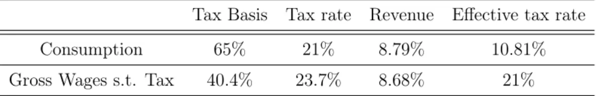
Table 1: VAT and ESSC in Portugal, year 2007

Tax Basis Tax rate Revenue Effective tax rate

Consumption 65% 21% 8.79% 10.81%

Gross Wages s.t. Tax 40.4% 23.7% 8.68% 21%

security contribution tax rate is 23.75 percent of the gross wage. These two

taxes generate a revenue of approximately 8.6 percent of GDP each. Table

1 shows the tax basis, tax rates, and effective tax rate, defined below, for

2007.16

A simple back-of-the-envelope calculation, keeping the tax basis fixed,

indicates that for each percentage point increase in the effective VAT rate,

the Government can decrease the ESSC rate by 1.6 pp and keep the revenue

unchanged. Equivalently a 2.47 pp of effective ESSC or a 1.53 pp of effective

VAT generate 1 pp of GDP of tax revenues. Of course the basis will change

after the tax swap and I have shown their qualitative path in the model

simulations. To quantify the effects of the proportional tax swap on the tax

basis and the trade balance, I estimate two Structural Vector Autoregression

to find the elasticities of private consumption and of the wage bill (the two

tax basis), and of exports and import (the trade balance), to a shock to the

16

(27)

effective VAT rate,τc in the model above, and to a shock to the effective social

security tax rate,τw in the model above. I estimate two distinct statistical

models, one for each tax rate shock, because Portuguese quarterly data only

exist since 1995 so that the number of observations is relatively small and

does not allow to estimate large models.

A shock to

τ

c

Empirically the effective tax rate on consumption is defined as

τc ≡

V AT P C =

�nc

s=1τspcscs+

�ni

s=1τspisis+

�ng

s=1τspgsgs

P C (12)

wherenj is the number categories in each type of expenditurej =c, i, g

(con-sumption, investment and government expenditure, see footnote 14), subject

to possibly different tax rates and pj is the price index of each category. A

change in any of the terms of 12 leads to a change inτc. I definea shock to the

effective rate any shock that changes τc but does not change

contemporane-ously the nominal expenditures in consumption, investment and government

consumption (and imports)17

. There are potential issues in the suggested

identification procedure. First I am not identifying the anticipated

com-ponent of the tax rate change but only the unexpected part of the shock.

Second total nominal expenditure in each aggregate demand component is

different from the nominal expenditure subject to taxation: about two-third

of consumption and only a small fraction of private investment and

govern-17

(28)

.17 .1 7 .17 .18 .1 8 .18 .19 .1 9 .19 .2 .2 .2 .21 .2 1 .21 vatrate vatrate vatrate .08 .0 8 .08 .1 .1 .1 .12 .1 2 .12 .14 .1 4 .14 .16 .1 6 .16 tc_sa tc_ sa tc_sa 1995q1 1995q1 1995q1 2000q1 2000q1 2000q1 2005q1 2005q1 2005q1 2010q1 2010q1 2010q1 quarter quarter quarter Effective rate Effective rate Effective rate General rate General rate General rate

Source: Eurostat, 2010

Source: Eurostat, 2010 Source: Eurostat, 2010 Effective and general VAT rates

Effective and general VAT rates

Figure 6: Effective and general VAT rates in Portugal. Source: Eurostat

ment expenditure are subject to VAT. Equation 12 also shows that to change

the effective rate the government can change the tax rates τs and/or change

the basis, nj 18. Figure 6 shows the seasonally adjusted effective VAT rate

together with the general rate.

The figure shows that when the general rate changes, the effective rates

changes in the same direction. However the effective rate exhibits a much

more volatile pattern characterized by a few large spikes. Some of the largest

spikes can be explained by a change in VAT legislation that did not alter the

18

Define the difference between nominal expenditure and the actual expenditure subject to the VAT as�j. For example in the case of consumption�c≡�

nc

s=1pcscs−P C. Therefore

the shock the effective rate will contain both changes in the different τs and changes in

(29)

Table 2: VAT history in Portugal

General Intermediate Reduced Effective tax rate

01.01.1995 – 30.06.1996 17% - 5% 10.9%

01.07.1996 – 04.06.2002 17% 12% 5% 12.3%

05.06.2002 – 30.06.2005 19% 12% 5% 13.45%

01.07.2005 – 30.06.2008 21% 12% 5% 14.7%

01.07.2008 – 30.06.2010 20% 12% 5% 12.3%

01.07.2010 - 31.12.2010 21% 13% 6% 12.9%

general rate. For example Table 2shows that the first large spike is in 1996q3

corresponds to the year in which an intermediate VAT rate of 12 percent was

introduced.

The previous discussion suggests that a careful narrative approach to the

VAT legislation in Portugal could be followed to construct a time series for

the effective VAT shock. Here I rely on the identification scheme suggested

above. For robustness, I estimate two SVAR, VAR 1 and VAR 2, containing,

real imports, nominal private investment, nominal government consumption,

nominal private consumption and the empirically measured effective tax rate

(VAR 1), or the actual general VAT rate (VAR 2). All variables except the

tax are in annual growth rates. The sample is 1996q3-2010q3, the VARs are

estimated with two lags and a dummy for the global financial crisis period.

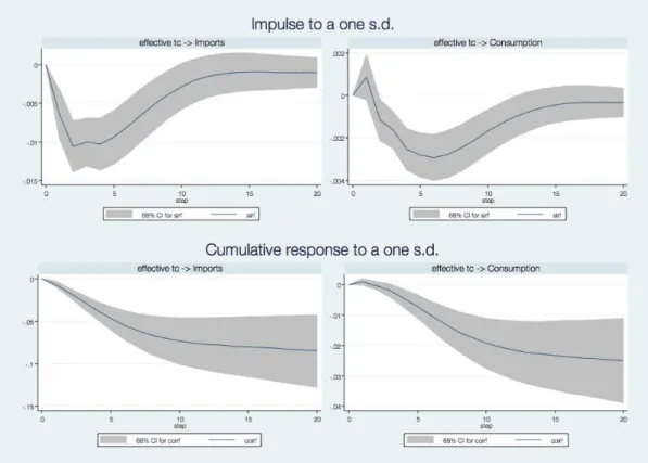
Figure 7 shows both the impulse and the cumulated responses of consumption

and imports to a one standard deviation of the identified VAT shocks together

with 68% confidence intervals for VAR 1.

The two shocks identified with the two alternative measures of VAT tax

(30)

(31)

Table 3: Percentage response to a one standard deviation increase inτc, CI 68%

Horizon τc onpc τc on m

2 years [-1.35,-2.1,-2.8] [-3.5,-6.27,-8.99]

5 years [-1.7,-3.4,-5.09] [-2.9,-8,-13.24]

itive shock, consistently with the benchmark model, decreases persistently

both consumption and imports. The results of VAR 2 are less precise

there-fore in the rest of the paper I use the results of VAR 1. The cumulative

responses show that a one standard deviation shock in effective VAT rate

decreases the level of nominal consumption (the VAT approximate basis) by

2 percent after 2 years and by 3.2 percent after 5 years. The same shock

ap-pears to have an even stronger effect on the real level of imports: 6 percent

after 2 years and 8 percent after 5 years. These elasticities appear to be very

large. Notice that the uncertainty on the effect is also large and that the

standard deviation of the shock is not identified. The lack of identification

of the structural shock standard deviation is common to the SVAR

litera-ture and does not allow to rescale the elasticities in terms of more practical

percentage change in the shock. Table 3 summarizes the results.

A shocks to

τ

w

Evidence on the effects of a change in τw is somewhat harder to identify as

(32)

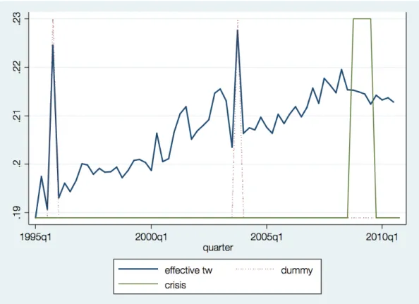
Figure 8: Effective SSC rate in Portugal. Source: Eurostat

the social security general rate19

. Figure shows the effective tax rate defined

as follows

τw ≡

SSC

Compensation−SSC =

�nw

s=1τwsWs

W (13)

where SSC are the social security contributions paid by the employers

and Compensation is the total compensation paid by the employers

inclu-sive of social security contributions. The effective τw exhibits an increasing

trend and two evident spikes. The trend corresponds to the widening of the

social security during the sample. The two spikes are due to above average

revenues in social security contributions during in the fourth quarter of 1995

19

(33)

and the fourth quarter of 2003. Again, following a narrative approach, these

two increases could be explained by new legislation passed at that time such

a more punitive stance towards evasion and the creation of a “revenue

min-imum d’insertion”. I nevertheless decide to control for the two spikes with

a dummy but results are not significantly affected by this choice. I define

a shock to the effective rate any shock that changes τw but does not change

contemporaneously the nominal wage bill W. The identification assumption

is subject to similar caveats than those expressed for the VAT shock. The

estimated VAR contains real exports, the nominal wage bill and the

effec-tive social security tax rate. Again all variables except the tax are in annual

growth rates. The sample is again 1996q3-2010q3, the VAR is estimated with

two lags, the dummy for the two spikes of 1995q4 and 2003q4 and a dummy

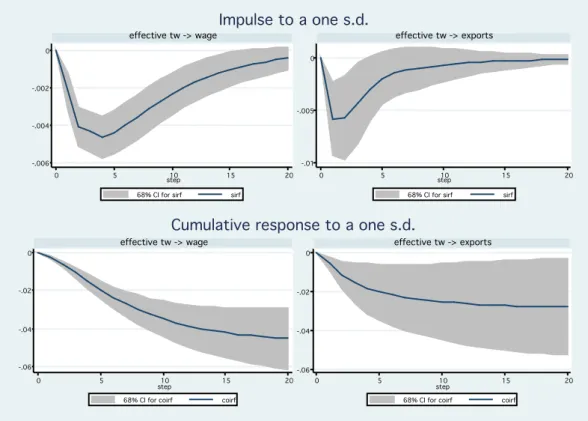
for the global financial crisis period. Figure 9 shows both the impulse and the

cumulated responses of the nominal wage bill and exports to a one standard

deviation of the identified τw shock together with 68% confidence intervals.

A positive shock decreases persistently both the wage bill and exports.

The cumulative responses show that a one standard deviation shock in

ef-fective social security tax rate decrease the level of the nominal wage bill

(maybe through lower employment) by 3 percent after 2 years and by 4.5

percent after 5 years. The same shock decreases the real level of exports by

2.3 percent after 2 years and 2.79 percent after 5 years. Again the confidence

intervals are large and the standard deviation of the shock is left unidentified.

(34)

-.006 -.006 -.006 -.004 -.004 -.004 -.002 -.002 -.002 0 0 0 0 0 0 5 5 5 10 10 10 15 15 15 20 20 20 step step step

68% CI for sirf

68% CI for sirf 68% CI for sirf

sirf

sirf sirf

effective tw -> wage

effective tw -> wage effective tw -> wage

-.01 -.01 -.01 -.005 -.005 -.005 0 0 0 0 0 0 5 5 5 10 10 10 15 15 15 20 20 20 step step step

68% CI for sirf

68% CI for sirf 68% CI for sirf

sirf

sirf sirf

effective tw -> exports

effective tw -> exports effective tw -> exports

Impulse to a one s.d.

-.06 -.06 -.06 -.04 -.04 -.04 -.02 -.02 -.02 0 0 0 0 0 0 5 5 5 10 10 10 15 15 15 20 20 20 step step step

68% CI for coirf

68% CI for coirf 68% CI for coirf

coirf

coirf coirf

effective tw -> wage

effective tw -> wage effective tw -> wage

-.06 -.06 -.06 -.04 -.04 -.04 -.02 -.02 -.02 0 0 0 0 0 0 5 5 5 10 10 10 15 15 15 20 20 20 step step step

68% CI for coirf

68% CI for coirf 68% CI for coirf

coirf

coirf coirf

effective tw -> exports

effective tw -> exports effective tw -> exports

Cumulative response to a one s.d.

Figure 9: The effect of a shock to the effective social security rate on wages and exports.

Table 4: Percentage response to a standard deviation shock inτw, CI 68%

Horizon τw onγx τw onγw

2 years [-0.6,-2.38,-4.17] [-2.52,-3.01,-3.77]

(35)

Discussion

I mentioned above that a better empirical model would estimate and

iden-tify the two shocks in a single statistical model. Typically the omission of

relevant information tends to bias estimates, and this is a serious concern

for what regards the magnitude of the estimated elasticities. Unfortunately,

leaving aside complications on the identification procedure, the number of

observations, 59 data points, is too small to obtain meaningful results from

the larger model. I also mentioned that the size of the identified shock is

left unidentified which does not allow to quantify the effect of a 1 percent

increase in the effective VAT rate on consumption and exports but only the

effect of a standard deviation increase. A narrative approach to the

construc-tion of the shocks would be useful to measure their size. Here I have to take

a stand on the relative size of the two shocks to be able to continue

meaning-fully the analysis. Figure 10 shows the first difference of the two empirically

measures effective rate. Their change (and their standard deviations) have

similar magnitude. I do not have a better metric than Figure 10 , therefore

I choose to assume that the two structural shocks have the same standard

deviation.

The empirical effects of the fiscal devaluation

Consider a 1 pp increase in τc. According to the simple back of the envelope

calculation to keep the tax revenue unchanged on impact τw can decrease

by 1.6 pp. Accordingly with the assumption that the two structural shocks

(36)

-.03

-.03 -.02

-.02

-.02 -.01

-.01

-.01 0

0

0 .01

.0

1

.01 .02

.0

2

.02 1996q3

1996q3 1996q3 2000q1

2000q1 2000q1

2003q3

2003q3 2003q3

2007q1

2007q1 2007q1

2010q3

2010q3 2010q3

quarter

quarter quarter

D.tc

D.tc D.tc

D.tw

D.tw D.tw

crisis

crisis crisis

dummy_tw

dummy_tw dummy_tw

(37)

0 0 0 50 50 50 100 100 100 150 150 150 million euro mi lli on e u ro million euro 0 0 0 5 5 5 10 10 10 15 15 15 20 20 20 quarter quarter quarter

Revenue balance after 1X tax swap

-2500 -2500 -2500 -2000 -2000 -2000 -1500 -1500 -1500 -1000 -1000 -1000 -500 -500 -500 0 0 0 million euro mi lli on e u ro million euro 0 0 0 5 5 5 10 10 10 15 15 15 20 20 20 quarter quarter quarter

Revenue balance after 10X tax swap

250 250 250 300 300 300 350 350 350 400 400 400 450 450 450 million euro mi lli on e u ro million euro 0 0 0 5 5 5 10 10 10 15 15 15 20 20 20 quarter quarter quarter

VAT revenues after 1x standard shock in tc

0 0 0 1000 1000 1000 2000 2000 2000 3000 3000 3000 million euro mi lli on e u ro million euro 0 0 0 5 5 5 10 10 10 15 15 15 20 20 20 quarter quarter quarter

VAT revenues after 10x standard shock in tc

-500 -500 -500 -400 -400 -400 -300 -300 -300 -200 -200 -200 -100 -100 -100 million euro mi lli on e u ro million euro 0 0 0 5 5 5 10 10 10 15 15 15 20 20 20 quarter quarter quarter

SSC revenues after 1.6x standard shock in tw

-3000 -3000 -3000 -2800 -2800 -2800 -2600 -2600 -2600 -2400 -2400 -2400 -2200 -2200 -2200 million euro mi lli on e u ro million euro 0 0 0 5 5 5 10 10 10 15 15 15 20 20 20 quarter quarter quarter

SSC revenues after 16x standard shock in tw

-.04 -.04 -.04 -.02 -.02 -.02 0 0 0 .02 .0 2 .02 .04 .0 4 .04 percentage percentage percentage 0 0 0 5 5 5 10 10 10 15 15 15 20 20 20 quarter quarter quarter Exp Exp Exp Imp Imp Imp

External balance after 1 standard tax swap

-.4 -.4 -.4 -.2 -.2 -.2 0 0 0 .2 .2 .2 .4 .4 .4 percentage percentage percentage 0 0 0 5 5 5 10 10 10 15 15 15 20 20 20 quarter quarter quarter Exp Exp Exp Imp Imp Imp

External balance after 10 standard tax swap

Figure 11: The empirical effects of a fiscal devaluation on tax revenues and the external balance.

the first consider the increase in 1 standard deviation of the effective VAT

shock coupled with a decrease of 1.6 standard deviation in the effective social

security tax shock, the second a 10 standard deviation increase in the VAT

shock coupled with a 16 standard deviation decrease in the social security

tax shock.

The estimated effect of τw on its own basis (wage) is relatively larger

than the effect of τc on its own basis (consumption), therefore Figure 11

shows that a fiscal devaluation that would maintain the tax revenue balanced

maintaining the tax basis unchanged, has a positive effect on the budget

(38)

the trade balance each standard deviation of the VAT shock decreases real

imports by 3.4 percent so that a 10 standard deviation increase is estimated

to decrease the level of imports by 34 percent. Further each 1.6 standard

deviation decrease in the SSC shock improves the level of real exports by

4.4 percent so that a 16 standard deviation decrease would increase exports

by 44 percent. Overall the empirical analysis appears to support both the

efficacy and the feasibility of a fiscal devaluation. Finally, to depart from

the quantification in terms of standard deviations I further assume that the

standard deviation of the two structural shocks is 1 pp (which corresponds to

effective rate standard deviation, but this is a poor justification) and consider

a decrease of the ESSC from 23.75 percent to 7.75 percent. In theory this

would achieve an instantaneous decrease of the labor costs of 16%. Tax

revenues would fall on impact by almost 7 percent of GDP. To keep the

revenue unchanged, the effective VAT rate should increase by 10 pp. This

increase in the effective rate is massive, but so too is the reduction in the cost

of labor. Table 2 suggests that the effective VAT rate could be increased from

11.4 percent to 21.4 percent by using the new general VAT rate on almost

every good. Considering the recent increase of the general rate from 21 to

23 percent, an almost uniform application of the latter rate could increase

the effective VAT rate by the order of magnitude required. The estimated

tax basis elasticities suggest that over time the revenue generated by the two

taxes will not deteriorate but actually improve. It is important to understand

that these numbers are conditional on the size of the shocks so that in practice

the uncertainty on the estimates of the relevant elasticities involved in the

(39)

0 0 0 .05 .05 .05 .1 .1 .1 IRL IRL IRL NLD NLD NLD LUX LUX LUX DEU DEU DEU AUT AUT AUT PRT PRT PRT SVK SVK SVK BEL BEL BEL ITA ITA ITA ESP ESP ESP FIN FIN FIN FRA FRA FRA DNK DNK DNK

Source: Eurostat, 2010 Source: Eurostat, 2010

Payroll as a share of GDP

Payroll as a share of GDP Payroll as a share of GDP

0 0 0 .02 .02 .02 .04 .04 .04 .06 .06 .06 .08 .08 .08 .1 .1 .1 LUX LUX LUX ESP ESP ESP ITA ITA ITA DEU DEU DEU BEL BEL BEL IRL IRL IRL FRA FRA FRA NLD NLD NLD SVK SVK SVK AUT AUT AUT PRT PRT PRT FIN FIN FIN DNK DNK DNK

VAT as a share of GDP

VAT as a share of GDP VAT as a share of GDP

Tax structure: average during 2000-2007

Figure 12: Tax revenues as a share of total tax revenues for VAT and payroll tax collection. The numbers shows are average shares from 2000 to 2007.

on the trade balance. Undoubtedly a permanent tax swap, as opposed to a

transitory one, would transform the tax structure of Portugal pushing it far

from the average European model, and make it similar regarding VAT and

ESSC to Denmark, where payroll taxes are around 3 percent and there is a

single VAT rate of 25 percent on virtually all goods and services20

.

To illustrate this point, Figure 12 shows that Portugal’s reliance on payroll

tax for generating tax revenue is just above the European average while VAT

appears to be more important than for the rest of the European countries for

20

(40)

generating tax revenues. The latter observation can only partly be explained

by a high general VAT in Portugal relative to the other countries: first,

Portugal does not have the highest VAT rate, and second, several reduced

VAT rates on relevant goods and services appear to be below other European

rate. For example, Figure 13 shows the rates on electricity and natural gas,

which appear to be much lower than in the rest of Europe.

In fact, I interpret part of the high dependence of Portugal on VAT

rev-enues as another symptom of excessive Portuguese consumption. Again the

departure from a “European model” would not happen in the transitory

ver-sion of the policy.

Conclusion

In this work I study the short run effects of a swap between a consumption tax

and a labor tax within a monetary union and perform an empirical analysis

of the tax swap on Portuguese data. The suggested tax swap is one of the few

policy left to individual EMU members to engineer a synthetic devaluation.

A transitory version of the tax swap has some attractiveness. A temporary

uniformization of the different VAT rates21

to the general rate, say for two

to four years, could generate the revenues to finance the initial cut in the

ESSC rate and allow the dynamic adjustment of lower consumption, higher

competitiveness, and higher employment to take place. If the policy is

suc-cessful, the larger ESSC tax basis would help to compensate the reduction in

consumption and probably allow again reducing the VAT rates on particular

21

(41)

0 0 0 .05 .05 .05 .1 .1 .1 .15 .15 .15 .2 .2 .2 .25 .25 .25 VAT VAT VAT Cyprus Cyprus Cyprus Luxembourg Luxembourg Luxembourg Malta Malta Malta Spain Spain Spain Germany Germany Germany Netherlands Netherlands Netherlands Slovak Republic Slovak Republic Slovak Republic France France France Austria Austria Austria Italy Italy Italy Slovenia Slovenia Slovenia Belgium Belgium Belgium Ireland Ireland Ireland Portugal Portugal Portugal Finland Finland Finland Greece Greece Greece Denmark Denmark Denmark

VAT general rate

0 0 0 .05 .05 .05 .1 .1 .1 .15 .15 .15 .2 .2 .2 .25 .25 .25 PetrolVAT PetrolVAT PetrolVAT Cyprus Cyprus Cyprus Luxembourg Luxembourg Luxembourg Malta Malta Malta Spain Spain Spain Germany Germany Germany Netherlands Netherlands Netherlands Slovak Republic Slovak Republic Slovak Republic France France France Austria Austria Austria Italy Italy Italy Slovenia Slovenia Slovenia Belgium Belgium Belgium Ireland Ireland Ireland Portugal Portugal Portugal Finland Finland Finland Greece Greece Greece Denmark Denmark Denmark

VAT on Petrol 2010

(a) VAT rates in Europe, general rate and petrol.

0 0 0 .05 .05 .05 .1 .1 .1 .15 .15 .15 .2 .2 .2 .25 .25 .25 NaturalgasVAT NaturalgasVAT NaturalgasVAT Luxembourg Luxembourg Luxembourg Portugal Portugal Portugal Italy Italy Italy Greece Greece Greece Ireland Ireland Ireland Cyprus Cyprus Cyprus Malta Malta Malta Spain Spain Spain Germany Germany Germany Netherlands Netherlands Netherlands Slovak Republic Slovak Republic Slovak Republic France France France Austria Austria Austria Slovenia Slovenia Slovenia Belgium Belgium Belgium Finland Finland Finland Denmark Denmark Denmark

VAT on gas 2010

0 0 0 .05 .05 .05 .1 .1 .1 .15 .15 .15 .2 .2 .2 .25 .25 .25 ElectricityVAT ElectricityVAT ElectricityVAT Luxembourg Luxembourg Luxembourg Portugal Portugal Portugal Italy Italy Italy Greece Greece Greece Ireland Ireland Ireland Cyprus Cyprus Cyprus Malta Malta Malta Spain Spain Spain Germany Germany Germany Netherlands Netherlands Netherlands Slovak Republic Slovak Republic Slovak Republic France France France Austria Austria Austria Slovenia Slovenia Slovenia Belgium Belgium Belgium Finland Finland Finland Denmark Denmark Denmark

VAT on electricity 2010

(42)

goods and services. Most importantly, the sharper reduction in consumption

would allow the Portuguese economy to start the much needed deleveraging.

On a broader note, I see the sophisticated use of the tax structure by

individ-ual EMU members as a possible substitute for more conventional automatic

stabilizers to external imbalances. The creation of fiscal tax rules in the spirit

of the “budget neutral” temporary tax swap described here could facilitate

and accelerate external adjustments with the eurozone as the prospects of a

deeper fiscal integration appear remote. Certainly the construction of these

new automatic stabilizers requires a great research effort in order to have a

more precise comprehension of their effectiveness and feasibility.

Appendix A

Model

Assume an economy with two countries in a monetary union, home (H) and

foreign (F). The home country is of sizen, while the foreign country is of size

1−n. The small open economy version of the model is obtained by taking

the limit n →0 after having solved the model. Technology and preferences

are the same across countries. In the following I describe the home economy

while the foreign which is completely symmetric is omitted. All foreign

vari-ables are denoted with an asterisk. The next two subsections describe the

firms and households problems together with the intratemporal optimality

conditions. The third subsection presents the intertemporal optimality

(43)

market clearing conditions.

Firms

The economy is composed of two two sectors, a tradable sector denoted by

T and a non tradable sector denoted by N. Workers are perfectly mobile

across sectors. Assume a continuum of firms indexed by i ∈ [0,1], each of

which produces a differentiated good with the following technology

Y_tx(i) =AtNtx(i)1 −a

, x=N, T (14)

whereYx

t (i)denotes the output of goodi, At is an exogenous technology

parameter, and Nx

t(i) is an index of labor input used by firm i and defined

by

Ntx(i) =

�ˆ 1

0

Ntx(i, h)

σw−1 σw dh

�_σwσw₋₁

, x=N, T (15)

whereNtx(i, h)is the quantity of type-hlabor employed by firmiin sector

x in period t. The parameter σw represents the elasticity of substitution

among labor varieties. The demand schedule for each labor type is obtained

by cost minimization

Ntx(i, h) =

�

Wt(h)

Wt

�−σw

Ntx(i), x=N, T (16)

for all i, h ∈ [0,1], where Wt(h) is the nominal wage for type h labor,

Wt =

�

´1

0 Wt(h)

1−σ_w

dh�

1 1−σw

is an aggregate wage index and Nx

t is firm’s

total employment. All firms face an isoelastic demand schedule (specified

(44)

given period independently of the time elapsed since the last adjustment.

Firms must pay a social contribution in the form of a proportional tax, τw,t,

on their wage bill.

Households

Assume a continuum of households indexed by h ∈ [0,1]. The household

seeks to maximize

Et

� ∞

�

s=t

U(Ct+s(h), Nt+s(h))

�

(17)

where Nt(h) is the quantity of labor supplied. Each household is

as-sumed to specialize in the supply of a different type of labor, also indexed

by h∈[0,1]. Furthermore, each household has some monopoly power in the

labor market, and posts the (nominal) wage at which it is willing to supply

specialized labor services to firms that demand them. Assume that for each

period only a fraction 1−θ_w _{of household, drawn randomly from the}

popu-lation, reoptimize their posted nominal wage. Under the assumption of full

consumption risk sharing across households, all households resetting their

wage in any given period will choose the same wage, because they face an

identical problem. Ct(h) is a composite consumption index

Ct(h) =

�

(1−γ)1s �CN

t (h)

�s−_s1

+γ1s �CT

t (h)

�s−_s1�

s s−1

(18)

where CN

(45)

given by a constant substitution elasticity aggregator

C_tN(h) =

� �

1

n

�_σn1 ˆ n

0

(cN_t (h, i))σ−σ1di

�_σnσn₋₁

(19)

where cNt (h, i) denotes the consumption by household h of good i ∈ [0,1]

denotes the good variety,n ∈[0,1]denotes the size of the domestic economy

(which corresponds to the type of goods it produces) andσn>1the elasticity

of substitutions between goods. In equation 18, the parameter s denotes the

elasticity of substitution between non traded and traded goods, γ denotes

the share of consumption allocate to traded goods and CT

t (h)is a composite

index of consumption of traded goods

C_tT(h) =�νλ1 �CH

t (h)

�λ−_λ1

+ (1−ν)λ1 �CF

t (h)

�λ−_λ1�

λ λ−1

(20)

whereCH

t (h) andCtF(h)are respectively an index of consumption of

do-mestic goods and foreign goods given by a constant elasticity of substitution

aggregator

C_tH(h) =

� �

1

n

�_σn1 ˆ n

0

(cH_t (h, i))σ−σ1di

�_σnσn₋₁

(21)

C_tF(h) =

� �

1 1−n

�_σn1 ˆ 1

n

(cF_t (h, i))σnσn−1di

�_σnσn₋₁

(22)

In equation 20 ν = 1 −(1− n)α where α ∈ [0,1] denotes the degree of

openness. The parameter σn > 1 denotes the elasticity of substitution

(46)

constraints of the form

(1 +τc,t)

�ˆ n

0

pH_t (i)cHt (h, i)di+ ˆ n

0

pN_t (i)cN_t (h, i)di+

ˆ 1

n

pF_t (i)cF_t (h, i)di

�

+Bt+1(h)+Et{Qt,t+1Dt+1(h)}+Mt+1(h)≤RtBt(h)+Dt(h)+Mt(h)+Wt(h)Nt(h)+Πt(h)+Tt(h)

(23)

whereτc,tis a proportional tax on on consumption, pxt(i), x=H, N, F are

the individual prices of each good,Dt+1 is the nominal payoff in periodt+1of

the portfolio of financial assets held at the end of period t (domestic financial

markets are complete to simplify the introduction of nominal wage rigidities

which requires insurance between workers to avoid income heterogeneity and

the departure from the representative agent),Bt+1is a nominal riskless bond,

Mt+1 is the quantity of money, Rt is the nominal gross interest rate on the

nominal bond, Wtis the nominal wage, Πt are the profits of the firms andTt

denotes lump-sum transfers/taxes. Qt,t+1 is the stochastic discount factor for

one-period-ahead nominal payoffs relevant to the domestic household. The

optimal allocation of any given expenditure within each category off goods

yields the demand functions

cHt (h, i) =

1

n

�

pHt (i)

PH

t

�−σ_n

CtH(h) (24)

cN_t (h, i) = 1

n

�

pN t (i)

PN

t

�−σ_n

C_tN(h) (25)

cF_t(h, i) = 1 1−n

�

pF t (i)

PF t

�−σ_n

(47)

for allh, i∈[0,1],PH t = � 1 n ´n 0 � pH t (i)

�1−σn

di�

1 1−σn

,PN

t = � 1 n ´n 0 � pN t (i)

�1−σn

di�

1 1−σn

andPtF =

�

1

1−n

´1 n

�

pFt(i)

�1−σ_n

di�

1 1−σn

are the price indexes for each category

of good. The optimal allocation of expenditure in tradable goods between

domestic and foreign implies

C_tH =ν

� PT t PH t �λ

C_tT (27)

C_tF = (1−ν)

� PT t PF t �λ

C_tT (28)

where PT = �ν�PtH

�1−λ

+ (1−ν)�

PtF

�1−λ�

1 1−λ

is a price index of

trad-able goods. Finally the optimal allocation of expenditure between tradtrad-ables

and non tradables is given by

C_tN =

�

Pt

PN

t

�s

(1−γ)Ct (29)

CtT =

�

Pt

PT t

�s

γCt (30)

where P = �(1−γ)�

PtN

�1−s

+γ�PtT

�1−s�

1 1−s

is the consumer price index

(CPI).

Intertemporal conditions

A firm reoptimizing in period t will choose the price p∗

t(i) (I have omitted

the superscript of the sector) that maximizes the current market value of the

(48)

associated with the problem above takes the form

∞

�

k=0

(ϑp) k

Et{Qt,t+kYt+k(i) (p ∗

t(i)−µpψt+k(i))}= 0 (31)

whereψt+k(i)≡ (1+τ

W t )Wt

(1−α)A_tN_t(i)−α is the nominal marginal cost andµp ≡

σ σ−1

is the desired firm’s markup in absence of of nominal rigidities. A household

resetting its wage W∗

t(h) in period t, maximize its utility while the wage

remains effective. The first order condition associated with the problem

above takes the form

∞

�

k=0

(βϑw)kEt

�

Nt+k(h)Uc(Ct+k(h), Nt+k(h))

�

W∗

t(h)

Pt+k

−µwM RSt+k(h)

��

= 0

(32)

where M RSt(h)≡ −(1+τ_Uc,t_c₍)_CU_tn₍_h(C₎_,Nt(h_t₍)_h,N₎₎t(h)) is the marginal rate of

substitu-tion between consumpsubstitu-tion and work and µw ≡ _σσ_ww−1 is the desired worker’s

markup in absence of of nominal rigidities. In addition to the wage setting

condition, the household’s problem also yields a conventional set of Euler

equations

Uc(Ct(h), Nt(h)) =βEt

�

Q−1 t,t+1

1 +τc,t

1 +τc,t+1 Pt

Pt+1

Uc(Ct+1(h), Nt+1(h))

�

(33)

Et{Qt,t+1}=

1

Rt

(49)

International prices

I assume the law of one price for tradables

P_tF(i) = P_tF∗(i);P_tH(i) =P_tH∗(i)

The real exchange rate

Qt=

P∗ t

Pt

and the terms of trade

St=

PF t

PH

t

Aggregate conditions

Given the assumed wage setting structure, the evolution of the aggregate

wage index is given by

Wt=

�

ϑwW1 −σw

t−1 + (1−ϑw)(W ∗ t)

1−σ_w�₁₋1_σw

while the assumed price setting structure implies

Pt =

�

ϑpP

1−σ_p

t−1 + (1−ϑp)(P ∗ t)

1−σ_p�

1 1−σp

Market clearing in the nontradables goods market requires

Y_tN(i) = C_tN(i) =

ˆ 1

0

cN_t (h, i)dh

(50)

requires

Y_tH(i) =C_tH(i) +C_tH∗(i) =

ˆ 1

0

cH_t (h, i)dh+

ˆ 1

0

cH_t ∗(h, i)dh

Letting aggregate output in each sector be defined asYx

t ≡

�

´n

0 Y

x t (i)

σp−1 σp _di

�_σpσp₋₁

it follows thatYN

t =CtN andYH =

�

ν�PtT

PH t

�λ�

Pt

PT t

�s

γCt+ 1 −n

n ν ∗

�_PT∗

t

PH∗

t

�λ� _P∗

t

PT∗

t

�s

γC∗ t

�

holds

for all t.

Market clearing in the labor market requires

Nt=

ˆ n

0

ˆ 1

0

N_tN(h, i)dhdi+

ˆ n

0

ˆ 1

0

N_tH(h, i)dhdi

The foreign country (rest of the union) is represented by a symmetric set

of equations.

Fiscal Policy

The fiscal authority is assumed to rebate tax income to households

τc,tCt+τw,tWtNt=Tt = ˆ 1

0

Tt(h)dh

Monetary policy

The central bank runs a common monetary policy for the two countries,

responding only to aggregate union-wide variables (U) that is represented by

a Taylor Rule

Rt= ¯R

�

PU

t

PU

t−1

�φp

(51)

whereφp denotes the feedback coefficient associated with the union wide

inflation gap (where the target is assumed to be zero) and �m

t is an iid

mon-etary policy shock.

Utility is assumed to have the following functional form

Ut=

C1−1σ

t

1− 1

σ

−χN

1+φ

t

1 +φ

The small open economy

The small open economy is derived taking the limn→0. The advantage of the

limit economy is to shut down all strategic interactions and allow to consider

Foreign (rest of the monetary union) variables as exogenous. The cost of

the limit economy is that with incomplete asset markets the steady-state

that depends on initial conditions (the initial net asset position) and the

equilibrium dynamics possess a random walk component. The assumption

of net foreign debt elastic interest rate allows to close the model.

References

[1] Vat rates applied in the member states of the european union. pages

1–27, Oct 2010.

[2] Bernardino Adao, Isabel Correia, and Pedro Teles. On the relevance

of exchange rate regimes for stabilization policy. Journal of Economic