HOW DO CURRENT TERM STRUCTURE
MODELS BEHAVE BEYOND THE LAST
LIQUID POINT?
A comparison of the DNS and Smith-Wilson methods
Catarina Moreira Batista
Nova School of Business and Economics
Maastricht University
Master Thesis supervised by:
Dr. Peter Schotman
Dr. João Pedro Pereira
January 2015
Abstract
This paper compares the popular Dynamic Nelson-Siegel (DNS) model with the
Smith-Wilson (SW) method for the extrapolation of yield curves within the scope of
the new regulation for pension funds and insurance companies, Solvency II. I have
focused particularly on the behavior of the models after the last liquid point (LLP) of
observable data. My main research shows that a longer LLP is beneficial at
extrapolating the yield curve as well as using a convergence period that relies on the
available data. I also found that the DNS model is more market consistent whereas the
SW method performs better fitting the available data and disregards the information
Table of Contents
Table of Contents ... 2
1. Introduction ... 3
1.1 Research Question ... 3
1.2 Literature ... 5
1.3 Methodology ... 6
1.4 Contribution ... 7
2. Literature Review ... 8
2.1 Traditional Term Structure Models ... 8
2.2 Current Yield Curve Forecast Models ... 10
2.3 Developments on the Solvency II Proposal ... 15
2.4 Model description ... 22
3. Research Design ... 26
3.1 Data ... 26
3.2 Determining the zero yield curve ... 28
3.3 DNS model – constant loadings and time-variant loadings ... 28
3.4 Smith-Wilson method ... 31
3.5 Comparison ... 32
4. Results ... 34
4.1 “Zero-coupon” yields ... 34
4.2 Dynamic Nelson-Siegel parameters ... 35
4.3 Smith-Wilson parameters ... 37
4.4 Estimated and extrapolated yields ... 37
5. Discussion ... 42
6. Conclusion ... 48
Bibliography ... 52
Annexes ... 54
1. Introduction
Without a doubt the term structure of interest rates has been the subject of much
debate, and interest rates themselves play a huge role for many economic agents –
they are a crucial macroeconomic variable, and they can be used as a monetary policy
instrument and a tool for determining the time value of money. Given the recent
events in financial markets many of the behaviors observed a decade ago have
changed. In Europe this was not only caused by the 2008 financial crisis but also by
the 2011 sovereign debt crisis, where one consequence was the appearance of yield
curves that were far from normal and the widening of credit spreads between Euro
area members. So from this point of view there is some interest in having a better
understanding of how the term structure behaves.
Moreover, this discussion has become of particular importance with the introduction
of new regulations for insurers’ and pension funds’ capital requirements in the scope
of Solvency II. In the current Solvency II directive, article 75 states that assets and
liabilities have to be valued with a market-consistent approach. At the same time, the
insurers and pension funds liable to this new regulation have liabilities that mature far
beyond anything traded in the market. So a issue appears: how can a reliable discount
curve be computed when liquid data is bound to lower maturities than those of the
liabilities to be discounted?
1.1 Research Question
The aforementioned issue brings me to my problem statement: “How do current term
structure models behave beyond the last liquid point?” with the last liquid point
(henceforth LLP) being defined as the maturity at which observed data is assumed to
lack of liquidity (thin market problem) or even inexistent instruments with those
maturities. The latest guidelines for implementation of Solvency II suggest the LLP
should be 20 years (EIOPA, 2014). Hence the goal of this thesis is to compare the
literature that models the yield curve and extrapolates it, in particular the dynamic
framework of the popular Nelson-Siegel model, to the method proposed in the
Solvency II guidelines (the Smith-Wilson method and the Ultimate Forward Rate).
To better understand the behavior of these models I will guide my research by
answering several sub-questions. Firstly, the Netherlands have applied regulations
similar to those in Solvency II and some studies have shown that possibly the chosen
LLP of 20 years might be too early and too abrupt (Rebel, 2012). There are two issues
here: one is the uncertainty on how long convergence should take between the market
data and a pre-determined interest rate level (in this case, the Ultimate Forward Rate).
Hence one of the concerns I would like to address is whether stability is achieved at a
maturity, T2, similar for both approaches. The second issue raised is whether the
20-year LLP is in fact the correct one – there is evidence that market data can be liquid
up to the 30-year point, so this is something I will also be testing.
When it comes to the models being compared there are also some concerns to be
answered. Eventually both models will converge to a constant level, but it would be
interesting to see how much the dynamic Nelson-Siegel derived curves would deviate
on the long-end compared to the Smith-Wilson curves. Furthermore when comparing
the models it is important to keep their purpose in mind – I am looking for a model
that can produce a realistic discount curve to use in the scope of Solvency II. So I will
Finally, I will also discuss the current level set for the Ultimate Forward Rate
(henceforth UFR) of 4.2%. The UFR is based off the idea of mean reversion but one
could argue on the feasibility of such a high level given the yields observable in the
market in the recent past as well as the inflation and economic growth expectations.
Thus I will have 4 main hypotheses guiding my research:
1. Is the maturity at which stability is achieved (T2) the same for the models
being tested?
2. How does the long-end of the curve compare in the NS model versus the
SW-UFR approach?
3. Which model do we expect to provide a superior approach for the purpose of
Solvency II?
4. Is the pre-determined UFR level of 4.2% realistic?
1.2 Literature
The Nelson-Siegel class of models in which I am focusing this paper builds upon the
traditional Expectations Theory of the term structure, which states that the yield of an
n-period bond will be an average of all “expected” yields over the next n periods. This
theory is a little simplistic and many have added to this proposition such as Cox,
Ingersoll, and Ross (1981) with the Preferred Habitat Theory, and Hicks (1946) with
the Liquidity Preference Theory.
The Nelson-Siegel model (Nelson & Siegel, 1987) aims to describe the yield curve
taking into account 3 factors – level, slope and curvature. Plenty of literature has
transformed the original model by incorporating some alterations like a no arbitrage
assumption, the introduction of extra explanatory factors (Svensson, 1995) or of
is particularly interesting as it introduces time variation to the original model while
having factors that carry some economical interpretation.
In the scope of Solvency II however the proposed methodology for the derivation of
the risk-free yield curve is the Smith-Wilson framework. Moreover EIOPA (2014)
suggests that the UFR be set at 4.2%, based on the assumption of 2.2% long-term
economic growth and 2% inflation, with an LLP of 20 years and a convergence period
to the UFR of 40 years for the Euro area. The upcoming implementation of this
proposal has renewed the interest in the yield curve especially in the countries where
similar regulations have been implemented such as Sweden and the Netherlands. For
example, Budiono (2012) tests the use of a variable UFR and a 30-year LLP on
pension fund performance, Chang and Li (2011) attempt extrapolation with a
volatility term structure, and Rebel (2012) finds that the 20-year LLP provokes an
unnatural behavior in the interest rate sensitivity of pension obligations.
1.3 Methodology
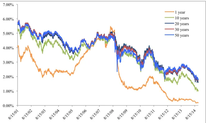
I have used Bloomberg to collect data on daily euro fixed-for-floating swap rates
between August 15th 2001 and November 19th 2014 maturing between 1 and 30 years.
My choice of the Euro swap rates is due to the fact that these new regulations will be
applied within the Eurozone even though other countries (like other European
countries and the US) are likely to face similar constraints in the near future. Having
said that, my analysis could be easily extended to other regions and countries. I ran
two estimations – one assuming an LLP of 20 years and a second one assuming data
is available up to 30 years.
The two models being compared are the dynamic Nelson-Siegel model and the
2006; Diebold & Rudebusch, 2013) because as it is a time series model and not just
cross sectional, it is a superior approach for forecasting over the original model as it
describes dynamic properties of the yield curve. My approach will be on a first step to
estimate the loading parameter 𝜆 from the data. Koopman, Mallee, and Van der Wel
(2010) have found that introducing a time-varying loading parameter and volatility
improves the fit of the model. I decided to see how the use of a time-variant factor
loading 𝜆 would affect my results. The Smith-Wilson method uses the available data
to exactly fit bond prices where data is available and to extrapolate them by using a
weighted average of the last observable data point and the pre-determined UFR. The
speed of convergence to this level is determined by the mean reversion parameter 𝛼,
which can be compared to 𝜆 in the DNS.
1.4 Contribution
Although there are many empirical studies using the Nelson-Siegel model or
extensions of it, the literature on ultra-long maturities is still scarce and as I have
discussed this is a subject of relevance for some economic agents. Research tends to
test such models with data on very liquid securities, such as bonds with maturities of
between 3-months to 10-years, leaving open the question of whether or not longer
termed securities could be used and if so when the last liquid point should be defined.
This is especially important when we start dealing with the need to have a
market-consistent discount curve that can value liabilities over 60 or 70 years. Thus, a study
of the models in the literature with this time span in mind could actively help shape
the decisions of these investors in the future. Furthermore, because interest rates are
so important both in financial markets and the real economy, and bond markets are
still developing at a rapid pace I expect this study could be helpful in shaping future
2. Literature Review
As explained the main interest of the thesis is to do a comparison of term structure
models currently available in the literature when they are used to extrapolate interest
rate yield curves at ultra-long maturities. To clarify, the term structure of interest rates
(or yield curve) shows the relationship between zero-coupon bond yields and their
term to maturity. When plotted, its shape can give valuable insight, for example,
about the expected path of future interest rates.
2.1 Traditional Term Structure Models
Before elaborating on the models that aim to model the term structure I will start out
by giving a brief overview of traditional yield curve theories. These are the basis for
all attempts to model the yield curve and in particular I find it important to mention
the motivations behind the two main streams of literature on traditional yield curve
models, the Expectations Hypothesis and the Liquidity Preference Hypothesis, as they
will help understand later on the results obtained. One of the most popular term
structure models in traditional literature is the Expectations Hypothesis having been
developed over most of the 1900’s, starting with Fisher’s proposition that investors’
expectations of the future spot rates affected current long rates. While this theory
can’t be pinpointed to one individual, Modigliani and Shiller (1973) provide a clear
description: “ [it] hypothesizes that in a world in which the future short-term rates are
not known with certainty, the current yield of an n-period bond can be expressed as
the very same function of the short rates currently “expected” to rule over the next n
periods”.
This hypothesis clearly has some limitations. Cox et al. (1981) state that it seems to be
the theory in its many formulations fails to hold under situations where interest rates
are stochastic. They test four interpretations to the theory: the local expectations, the
return to maturity, the yield to maturity and the unbiased expectations where the latter
two overlap. It seems most of these formulations are lacking due to failing to realize
that even in the presence of risk neutrality bonds have a term or risk premium.
The first criticism in the literature came from Hicks (1946) who added to this
proposition by introducing the concept of a risk-premium. He builds upon Keynes’
Liquidity Preference hypothesis that rates are determined partially by default risk and
partially, on the long term, by uncertainty of future interest rates. He agrees that there
is such a premium and adds to the original Expectations Hypothesis by saying that the
long-term rate will generally exceed the average of the expected future spot rates by
this risk/liquidity premium.
This framework proposed by Hicks’ – the so-called Liquidity Preference model – can
be considered a special case of the Preferred Habitat theory (Cox et al., 1981), where
it is hypothesized that all investors have a preferred maturity in which they want to
invest in (for example due to availability of funds for that time frame) but that
investors may be enticed to invest outside of their preferred habitat due to higher
expected returns. Thus the Liquidity Preference model could be considered the case in
which all investors have a habitat that coincides with the shortest holding period.
Putting it in these terms they interpreted the investment habitat preference as a risk
rather than a time preference – investors who are less risk averse will demand positive
term premiums while those who are more risk averse are fine with a negative
premium. This interpretation seems to be more close in hand with reality – investors
as bond markets are functional and allow for trading of securities (whether or not the
market is liquid enough should be incorporated in the premium).
I found it also interesting to point out that using the Liquidity Preference model there
is evidence supporting the fact that past real interest rates and rates of inflation were
the main variables containing information about future rates (Modigliani & Shiller,
1973). In particular when plotting results it’s possible to see that (a) the short-term
rate’s lag structure was more characterized by extrapolative tendencies implying
rational expectations, and (b) when forecasting the very short-term rates (for next
quarter) information on the current rate was more important while the longer-term
rates weighed more heavily on past information up to some years back and less so on
the current rate. Modigliani and Shiller (1973) also found that the real rate of interest
was strongly associated with current inflation, and that inflation itself was mostly
impacted by its own past levels, having a lag structure with a strong regressive
component.
2.2 Current Yield Curve Forecast Models
Thus far I have presented the main theories that have shaped the later development of
the literature on the term structure. They provide some insight on how we can expect
the term structure to evolve and what variables may play a role in shaping future
interest rates. These are the basis for most of the literature that came afterwards when
trying to address the problem of modeling the term structure of interest rates. This
problem can actually be split into two: one is the concern with fitting the yield curve
to empirical data, and the other determining what will be the evolution of the curve
Initially the focus of this literature was on affine term structure models, which give a
closed form solution to bond pricing by using an affine relationship between the spot
rate and the state variables. They started out by being single factor models, such as the
seminal works of Vasicek, and Cox, Ingersoll and Ross. To illustrate, Cox, Ingersoll,
and Ross (1985) derived a single factor model based on general equilibrium where the
traditional theories are incorporated by considering expectations about future events,
risk preferences, characteristics of other investment alternatives, as well as investors’
specific preferences on consumption timing. It is assumed that there is one source of
market risk and this drives the evolution of interest rates, which follow a diffusion
process. This type of assumption, usually present on single factor models, can be
simplistic because by having the spot interest rate as the only explanatory factor it is
inherent that rate changes would be perfectly correlated along the curve. Furthermore,
with a single factor it is unlikely that there would be enough explanatory power to
extrapolate yields beyond the last liquid point, being the model more applicable to
short-term rates. There are also some multi factor models still within the affine class –
one work worth noting in is that of Duffie and Kan (1996) for the generalization of
the many models of this type in the literature. Nevertheless, it has been shown that
this class of models – affine term structure models – are not very good at
out-of-sample estimation, and actually do not outperform a random walk (Duffee, 2002).
Another stream of literature was concerned with ensuring a no-arbitrage condition
when modeling the term structure of interest rates. Hull and White (1990) and Heath,
Jarrow, and Morton (1992) are important examples of such contributions, where the
approach was cross-sectional instead of a time series, modeling the yield curve to fit
perfectly at one specific point in time. While having an arbitrage-free model is
lacking time dynamics and not offering a way to extrapolate the term structure
unfortunately.
On the literature of term structures of interest rates there is also the Nelson-Siegel
(henceforth NS) model which takes a more empirical rather than theoretical approach
to yield curve modeling, being able to fit yield curves of diverse shapes (humped,
S-shaped, inverted and monotonic). At its core it still has the Expectations Hypothesis
from the idea that forward rates, as forecasts of spot rates, would be the solution to the
differential equation that produces the spot rate. In the model proposed by Nelson and
Siegel (1987) the spot rate for the maturity τ-periods ahead is given by
𝑅 𝜏 = 𝛽!+𝛽 !
1−𝑒− 𝜏𝜆
𝜏 𝜆
+𝛽
!∙
1−𝑒− 𝜏𝜆
𝜏
𝜆
−𝑒− 𝜏𝜆
Where λ, β0, β1 and β2 are the parameters to be estimated that contain information on
the level, slope and curvature of the curve. These parameters can be seen as having a
different contribution depending on maturity – β0 can be seen as the long-term
component as it is a constant that does not decay to 0 in the limit, β1 has a large
contribution at short term maturities but decays rapidly to 0 given its exponential
term, and β2 when plotted against time to maturity has a shape similar to a bell, thus is
more of a medium term driver. This model benefits from being parsimonious and
from its simplicity, although it might under some circumstances not yield a perfect fit.
It’s also important to note that whether or not the model fits perfectly the data is not
necessarily correlated with it’s forecasting ability, for example McCulloch (1971)
develops a model using a cubic spline that can accurately fit the data but this type of
bounded at β0 when maturity is large and at (β0 + β1) for the instantaneous rate.
Moreover, when defining λ (which when small has a better fit at low maturities due to
rapid decay) we could choose to minimize the error term of each dataset but better
results are obtained when this is set to fit across the entire sample without great loss
of precision.
One important contribution to this model came from Svensson (1994), who adds an
additional parameter to the original NS framework to improve fit especially when the
data has irregularities (he studies Sweden’s data in the period of 1992-1994). In light
of this he includes a second curvature term, with two extra parameters, β3 and λ2, to
provide a better fit in particular at the end of the curve where data is scarcer and hence
where the NS model struggled to be flexible enough. The ECB uses the Svensson
version of the model when fitting its own yield curves and the parameters are
published daily on its website.
More recently the literature on yield curve modeling seems to have flourished from
the original NS framework especially after Diebold and Li (2006) and Diebold,
Rudebusch, and Boragan Aruoba (2006) dynamic factor model linking the original
NS factors to macroeconomic variables thus giving them some intuitive interpretation.
Concretely, Diebold et al. (2006) introduce variables such as inflation, the real
economic activity and the monetary policy instrument. Diebold and Li (2006) test the
model’s (henceforth DL) ability to forecast and find that it performs well in-sample
and out-of-sample for long maturities. Their 1-month-ahead forecasting results are
disappointing but they find that it improves dramatically after the 6-month-ahead
horizon. Moreover the DL model replicates the five stylized facts of the yield curve:
the average yield curve (i) is increasing and concave; (ii) assumes a variety of shapes
so; (iv) typically has a short end more volatile than the long end; and (v) its long rates
tend to be more persistent than its short rates. They base their approach on imposing
structure based on simplicity and parsimony such that it enhances the out-of-sample
forecasting ability of the model even if it means the in-sample fit will be slightly
deteriorated for lack of model flexibility. Nevertheless, Pooter (2007) finds that when
using a four-factor model based on Svensson’s model or the NS extension of Björk
and Christensen (1999), the out-of-sample results are satisfactory and the in-sample
fit is better than the three factor model when looking at the root mean square
prediction errors (RMSPE).
Koopman, Mallee, and Van der Wel (2010) take the DL dynamic model and introduce
time-varying factor loadings and time-varying volatility. They find evidence that both
extensions significantly improve the fit of the dynamic NS model (henceforth DNS).
Furthermore they show that not only is the assumption of a constant λ not the most
accurate, when it is used as a latent factor it is highly persistent and affects the
dynamics of the slope and curvature factors.
One other interesting addition to the class of DNS models is the condition of no
arbitrage put forward by Christensen, Diebold, and Rudebusch (2011), thus
introducing the class of arbitrage-free NS models which are affine arbitrage-free term
structure models with the DNS factor loading structure. This allows to bridge the gap
between the class of affine models that is theoretically rich but empirically lacking,
with the DNS which empirically works well but lacks in theory. Nevertheless it will
not be very useful for this case as the adjustment made causes very long-term rates to
converge to minus infinity due to the presence of a unit root in the level factor (Balter,
2.3 Developments on the Solvency II Proposal
Laying out these yield curve modeling frameworks is motivated by the recent debate
on the technical aspects of the currently still under work new directive for pension
funds and insurance companies operating in the European Union – the Solvency II
proposal which is supposed to come into force in January 2016. The objective of the
proposal is not only to harmonize these institutions across the European market but
also, and more importantly, to enforce certain guidelines for minimum capital
requirements (MCR) and solvency capital requirements (SCR). The technical debate
comes in where there is a need to discount assets and liabilities to compute these
requirements. This includes using market data when available and computing best
estimates that accurately reflect the risk present when direct market data is not
available (Steffen, 2008). The European Insurance and Occupational Pensions
Authority (henceforth EIOPA) has conducted several field-testing exercises –
Quantitative Impact Studies (QIS) – of Solvency II, the latest of which was QIS5 on
insurance institutions (thus far occupational pensions have only been subject to one
QIS in 2012).
The Committee of European Insurance and Occupational Pensions Supervisors
(henceforth CEIOPS) issued a final letter of advice for the implementation of
Solvency II Level 2 (CEIOPS, 2009) where they make some interesting
considerations. First and foremost, in this document CEIOPS points out that the
desired characteristics of the instrument in which the risk-free interest rate term
structure is based on are (i) having no credit risk; (ii) being realistically achievable by
all insurers; (iii) being reliable; (iv) being highly liquid for all maturities (closely
related to its reliability); (v) having no technical supply/demand biases; and (vi) being
extrapolation method in complying with the mentioned qualities, in particular realism,
and producing sufficient financial stability once it will be used in discounting the
value of liabilities that are due very far in the future. The further in the future the
liabilities are, the larger the impact of the discount rate used on their present value,
hence the importance of having some stability and adhering to the insurers’ reality. In
regards to credit risk they argue that government bonds (with triple-A rating) are safer
than swap contracts posing less credit risk, and thus they should always be preferred
as an instrument over the latter. This has changed after the sovereign bond market
events that occurred after the publication of this letter – in the latest technical
provisions issued by EIOPA, it is recommended the use of swap rates. Using the swap
rate is particularly useful if there are inequalities within the same currency, as is the
case within the euro area where the swap rate will be available for all member states
more equally than government bonds, which can have quite big spreads among them
(i.e. central vs. southern Europe sovereigns).
Some of these concerns were answered in the calibration documents for QIS5
(EIOPA, 2010b) where the Smith and Wilson (2001) method and Ultimate Forward
Rate (henceforth UFR) approach were first proposed for extrapolation beyond the last
liquid point (henceforth the LLP). In the previous field exercises the risk-free term
structures had been provided. As of April 2014, EIOPA (2014) has disclosed the
technical specifications for the preparatory phase of Solvency II implementation
which detail the proposed methods for calculation of the risk free term structure,
including the volatility adjustment, are detailed. In this document EIOPA defines the
UFR to be “the percentage rate that the forward curve converges to at the
pre-specified maturity” and, for a given currency, it incorporates the appropriate inflation
UFR will be 4.2%, a result of 2% inflation rate and 2.2% long-term growth rate.
Another important concept is that of the speed of convergence to the UFR,
represented by the α parameter in the Smith-Wilson method and which also
determines the smoothness of the curve. The higher the α the bigger the weight of the
UFR (hence faster convergence), while a lower α gives more weight to the market
data.
In terms of the use of the swap rate as the preferred instrument for the term structure
derivation, it is also important to point out that it should be adjusted accordingly for
credit risk (EIOPA, 2014). Specifically, there is credit risk embedded when the rate
on the floating leg of the swap is determined which depends on the credit quality of
the banks involved in the deal. The adjustment should be done as a fixed deduction
across all maturities and in the amount of the spread between these rates and the
overnight indexed swap rates of matching maturity.
Although modeling yield curves is a much debated topic, when it comes to
extrapolation at maturities beyond those provided in financial markets for the purpose
of Solvency II there is not much empirical work done on the matter. Throughout my
research I have found that much of what has been written on the subject stems from
the countries that have been early on adapters of a similar regulation, such as Sweden,
the Netherlands, and Denmark.
Budiono (2012) proposes an alternative calibration to the 20 year LLP and 4.2% UFR
by using a LLP of 30 years instead and a variable UFR based on market rates. She
finds this would significantly improve pension fund performance in terms of funding
In an attempt to improve how required capital for interest rate risk was computed
within the scope of Solvency II, van Beers and Elshof (2012) have used cubic
Hermite splines to interpolate spot rates. They argue that in this way the term
structure will better reflect the stress shocks implemented and the convergence to the
UFR. When using this method each set of neighboring spot rates is interpolated by
using a linear combination of Hermite functions, and so it is expected that it will not
only assure the term structure smoothness but also that the term structure can assume
realistic shapes. They find that this method would be particularly useful for complex
insurance products, whereas simple liability portfolios like immediate annuities work
relatively well under the simplistic assumptions proposed by EIOPA.
Faced with the problem of illiquidity beyond 10 years, little observable data and
potentially spurious short-term rates, Chang and Li (2011) extrapolated a volatility
term structure for Taiwanese data instead of the usual bond price term structure. By
showing the decay in the volatility of long-term forward rates, deriving a volatility
term structure can help determine the speed of convergence to the UFR. Their
formulation used a GARCH and a T-GARCH to estimate volatility and then fitted the
term structure based on Vasicek (1977), using optimization constraints consistent with
EIOPA (2010b). While Liu (2008) derived the theoretical volatility by setting the
forward rate from t-1 to t periods ahead to the proposed UFR, Chang and Li instead
fitted their term structure directly for a set of parameters that allowed the curve to be
extrapolated to the UFR. They found that using their proposed GARCH model the
term structure would converge more rapidly to the UFR than by using the QIS 5
method. As the Smith-Wilson method fits observed data directly this could be a
One of the pointers guiding my research was whether or not the maturity at which
stability was achieved (T2) would be the same for the models I’m testing. EIOPA
(2014) suggests the convergence period will depend on the country to which the
method is being applied, suggesting 40 years for the Euro area with an LLP at 20
years. This means that after the 20 year mark, rates are a weighted average of the last
observed forward rate and the pre-set UFR for a period of 40 years finally converging
to the 4.2% UFR. In the DNS model, on the other hand, the curve will converge to the
level parameter dependent on the decay parameter λ, which is estimated using the
available data. In particular, following from Koopman et al. (2010) results, my guess
would be that using the DNS model with a time variant decay parameter should be a
better reflection of the available data than the assumed T2, thus my first proposal
emerges:
Hypothesis 1. Using a decay parameter dependent of the observed data yields a better
extrapolation than a pre-defined one.
Moreover, Rebel (2012) critics EIOPA’s proposal by arguing that one of the flaws of
the UFR Smith-Wilson methodology is its abrupt disregard for market data beyond
the last liquid point of 20 years. Is there any evidence that liquidity declines
significantly after the 20-year mark? Provided secondary market trading of both
sovereign bonds and interest rate swaps is over-the-counter, it is not easy to answer
this question. If trading volume is used as a loose proxy for liquidity we can see in
figure 1 that, in fact, while there is a significant peak in trading volume around the
ten-year mark (possibly due to market segmentation), the German bonds maturing in
30 years still have a fairly high weekly trading volume (about 130 000 millions USD).
This is not by any means sufficient proof that the market data for such long maturities
there any concrete proof for the 20-year last liquid point. At most we could argue that
there is sufficient market liquidity up to ten years and then it significantly declines.
We can then weigh what the trade-off would be between on the one hand using less
data points but extremely reliable ones, or on the other hand, using more data points
but without certainty that they are completely unbiased.
Hence I consider it would be of value to test whether there are significant differences
on the extrapolation when using available data up to 30 years and propose the
following:
Hypothesis 2. An LLP of 20 years is inadequate and using the available liquid market
data up to 30 years improves extrapolation results.
My following question would be on how much the curves from the DNS model
deviate from the fixed UFR on the long-end. Clearly, the level factor will predominate
in the long run while the others will decay (Diebold & Rudebusch, 2013) making the
curve stable. However it would be interesting to see whether the DNS curves have a
Figure 1: Trading volume in German Bunds’ secondary market in the week 14/11/14 to 21/11/14, in millions USD. (Source: Bloomberg)
significant amount of variation at the long end when compared to the constant UFR.
This of course will depend on the decay parameter λ as it will determine the speed of
convergence on the DNS model. Balter et al. (2014) extrapolate curves using the NS
model (with an estimated λ set constant) and the SW method, finding that both
provide a smooth curve beyond the LLP of 20 years. The SW curve lies above the NS
due to the convergence to the UFR of 4.2%. I would like to test whether I find the
same when using a time variant λ or not.
When attempting to compare both models another question arises: which model do
we expect to provide a superior approach for the purpose of Solvency II? It is not
clear. From what has been discussed thus far, I would expect the following:
Hypothesis 3. The SW-UFR model will provide a better fit in-sample and the DNS
model a better out-of-sample extrapolation.
If this is true, how can we evaluate this trade-off? By using the available data, the
DNS provides a more realistic discount curve on the long end, however it should be
harsher for pension funds funding ratios when rates reach extremely low levels, as is
the case now. On the other hand precision in fitting the curve at shorter maturities (i.e.
before the set LLP) is not as good in the DNS as it is in the SW-UFR. As it has been
previously discussed, pension funds have liabilities with maturities beyond the LLP
(thus out-of-sample), so should my hypothesis be confirmed, it would be preferable to
have a better out-of-sample fit at the expense of a slightly worse in-sample fit.
Finally, is it possible to say that the UFR set level of 4.2% is realistic? For one, it is
arguably inconsistent with the current reality of interest rate markets. As it can be
seen from figure 2, yields at the longer-term maturities have been significantly
that it would be to a mean of 4.2%. The Netherlands UFR Committee (2013)
recommends that the UFR is set on the average of the 20-year forward rates of the
previous 120 months, which at the end of July 2013 would have yielded a UFR of
3.9%.
2.4 Model description
To research these issues I will be comparing the Dynamic Nelson-Siegel model
(Diebold & Rudebusch, 2013) with the proposed SW-UFR method. The
Smith-Wilson method is outlined in the Solvency II technical provisions (EIOPA, 2014).
The price of a zero-coupon bond is defined as a function of coupon bonds as
𝑃 𝜏 = 𝑒!!"#∗! + 𝑧!
!
!!! ∗
𝑐!,!
!
!!! ∗
𝑊 𝜏,𝜏!
Where 𝑧! is a set of parameters to be estimated with N observed data points
maturity-wise, and 𝑐!,! stores the information on the cash-flows paid for a given t bond at a
Figure 2: European Triple-A Government Bond Spot Yields, 20-year maturity. (Source: ECB Statistical Data Warehouse) 1.00%
1.50% 2.00% 2.50% 3.00% 3.50% 4.00% 4.50% 5.00% 5.50%
given n maturity. The W function, which can be seen as the equivalent to the loading
matrix in the NS model, is defined as
𝑊 𝜏,𝜏! =𝑒!!"#∗!!!!
∗ 𝛼∗min 𝜏,𝜏! −𝑒!!∗!"#!,!!
∗𝑠𝑖𝑛ℎ 𝛼∗min (𝜏,𝜏!)
The variables 𝜏 and 𝜏! store the information on maturities across the whole data set.
The first, 𝜏, can be seen as the maturity on a given bond so it corresponds to the rows
of the W function. The latter, 𝜏!, contains information on the maturities at which
coupons are paid, so it maps the columns of W. Lastly, 𝛼 is a pre-set mean reversion
parameter that determines the speed of convergence. Due to the symmetry of the W
function and being close to 0 when the maturity variables 𝜏 and 𝜏! are very large, it is
clear that it will converge to the UFR. Moreover on the liquid part of the curve it will
exactly fit the data available, while after that last liquid point, here determined by the
chosen N, the yields will be constructed based on the data points available and the
pre-determined continuously compounded UFR. In this model the idea is that the
price function 𝑃 𝜏 is assessed as a linear combination of !! 𝑐!,!
!! ∗𝑊 𝜏,𝜏! , which
can be compared to the NS model in the sense that it assesses the forward rate
function as a sum of the three different parameters (level, slope and curvature).
It is also important to clarify that the yield curve, the forward rate curve and the
discount curve are all related and thus easily interchangeable (Diebold & Rudebusch,
2013). The yield curve is related to the forward curve by
𝑦 𝜏 =1
𝜏 𝑓 𝑢 𝑑𝑢
!
!
with 𝑓 𝜏 =−𝑃
! 𝜏
𝑃 𝜏
Where 𝜏 is the time to maturity, 𝑦 𝜏 is the continuously compounded yield and 𝑃 𝜏
The Dynamic Nelson-Siegel model as described in Diebold and Rudebusch (2013) is
similar to the original model except that it introduces useful time dynamics to the
parameters. This is achieved by considering instead of a cross sectional projection of
𝑦 𝜏 , a time-series dimension for a given 𝜏, where the parameters 𝛽!,!, 𝛽
!,! and 𝛽!,!
become the variables.
𝑦 𝜏 =𝛽!
,!+𝛽!,!
1−𝑒!!"
𝜆𝜏 +𝛽!,!
1−𝑒!!"
𝜆𝜏 −𝑒
!!"
It relies on dynamic factor structure which is usually satisfied by financial data. As
previously mentioned, the factors 𝛽!,!, 𝛽!,! and 𝛽!,! have meaning – each will impact
different maturities of the term structure, long, short and medium-term respectively –
and can be seen as level, slope and curvature factor loadings.
The two models, the DNS and SW-UFR, are quite different in the way they are
formulated. For extrapolation, on the one hand the SW-UFR method relies on the last
known observation (at the LLP) and on the set UFR and the curve is created based on
a weighted average of both for the period of convergence. On the other hand, the DNS
method uses all the observed data to fit a curve and then uses the factor loadings to
extrapolate the remainder of the curve beyond the LLP. But apart from this, both
models have similar inputs. In the NS class of models we can read 𝜆 as being the
decay parameter that determines the maturity at which the factor loading on 𝛽! (the
curvature factor) is at its maximum. It can thus be seen as the T2 used in the UFR
model, as it marks the point at which the curve technically stabilizes. In DL 𝜆 was
fixed at a predetermined value (at 16.42 a value such that the maximum would be
reached at a 30-month maturity), whereas in Pooter it was estimated and then set
in the DNS model, we know from its formulation that in the very long-run it will
stabilize at𝛽! so it can be seen as the UFR in the DNS.
So in summary, to address the issues identified, I will use the described models in 3
different ways: (i) by estimating the models as described, using an LLP of 20; (ii)
using instead an LLP of 30 for both models; and (iii) by comparing the results
3. Research Design
The outline of my methodology is as follows: I first started by interpolating the yield
data available up to 30 years. As proposed in EIOPA (2014) the swap mid rate will be
used for deriving both the DNS and SW-UFR curves. Then, after deriving the swap
zero yield curve, I’ve fitted both the DNS and the SW-UFR models to that data and
then followed each model’s specifications in order to be able to extrapolate beyond
the assumed last liquid point of 20 years. The DNS and SW-UFR will be calibrated in
very different ways. In the case of the DNS I start with an initial estimation using a
pre-determined 𝜆 and then I fit the data using maximum likelihood estimation and a
Kalman filter. On the other hand for the Smith-Wilson method only simple matrices
calculations are needed. I went through this procedure a second time using the
available data up to the 30-year point. Finally I compared the results obtained.
3.1 Data
For the data collection I used Bloomberg and obtained the daily vanilla interest rate
swaps fixed-for-floating Euro mid rates for the period of August 15th 2001 to
November 19th 2014. This totals to 3453 observations. Although data for shorter
termed swaps is available before August 15th 2001, this is the first observation I have
for some of the longer maturities so in an attempt to harmonize the sample I chose
this start date. For each date, rates were obtained for swaps with time to maturity of
1-year through 30-1-years, as well as swaps maturing in 40 and 50 1-years. The swaps in
question have semi-annual settlement, tied to the six-month Euribor, and are quoted
on a 30/360 day-count. The evolution of some of these rates over the sample period
These swap rates are established as the midpoint between the bid and ask prices for
contracts where the counterparties exchange fixed interest rate cash flows for floating
cash flows, and vice versa. Thus at inception a swap does not involve any exchange of
money, it is a zero net cash flow, and so it’s value at that time is zero (Veronesi,
2010). This characteristic strongly reduces the risk involved in a transaction
(particularly counterparty risk) and that is why swaps have become such an important
instrument after the financial crisis of 2008. Knowing this the swap rate, 𝑠, can be
expressed as
𝑠= 𝑛× 1−𝑍 0,𝑇!
𝑍 𝑂,𝑇! !
!!!
Where 𝑍 0,𝑇 are discount factors and there are cash-flow payments at times j
through M, the maturity of the swap.
Figure 3: Evolution of fixed-for-floating Euro swap rates for swaps maturing in 1, 10, 20, 30 and 50 years. (Source: Bloomberg)
0.00% 1.00% 2.00% 3.00% 4.00% 5.00% 6.00% 7.00%
3.2 Determining the zero yield curve
As explained the first step in constructing the yield curve will be to bootstrap from the
Euro swap mid-rates, the remaining maturities in the liquid part of the curve (Smith,
2012). However I am interested in the zero yield curve, so I have to transform the
swap rates obtained, which for maturities over one year include cash flows (like a
coupon bond), into zero yields. In order to do this, we look at the swap rates as if they
were the coupon rate on a par bond in order to extract the unknown spot rates. The
one-year spot rate, 𝑅 0,1 , will be the same as the one-year swap rate, s1. For the
following maturities, the continuously compounded 𝑅 0,𝑀 can be obtained from
100%=
𝑠 ! 𝑒! !,! ∗!
!
!!!
+ 𝑠
!+100%
𝑒! !,! ∗!
In order to do this I used Matlab to extract the vector of 𝑅 0,𝑀 for each of the
observation dates by finding first the discount factors and then transforming them to
spot rates by the below relation.
𝑅 𝑡,𝑇 =−
𝑙𝑛 (𝑍 𝑡,𝑇 )
𝑇−𝑡
3.3 DNS model – constant loadings and time-variant loadings
Starting off with the parameterization of the DNS, there are several approaches that
could be used for its estimation: a two-step process, a maximum likelihood estimation
(using state-space representation and a Kalman filter), or even Bayesian analysis (in
conjunction with Monte Carlo). While the two-step DNS approach by using linear
regressions constitutes a simple and numerically stable method, it does not allow to
Thus I have decided to use the more precise maximum likelihood estimation
(henceforth MLE) with a Kalman filter, also known as the one-step DNS, and since it
can be sensitive to the initial parameters I have used prior to its estimation the
two-step approach to establish a parameterization that is close to the one I’m looking for.
For the initial two-step, or cross-sectional, approach I set lambda at 0.5 which is a
good estimate when using yearly data. Then I performed a simple ordinary least
squares estimation. The parameters obtained were then used for the starting values in
the estimation of the state-space model. Following Diebold and Rudebusch (2013) the
DNS yield curve can be transformed into a state-space representation of the model
denoting the β parameters as level, slope and curvature to emphasize their meaning.
𝑦! 𝜏 = 𝑙!+𝑠!
1−𝑒!!"
𝜆𝜏 +𝑐!
1−𝑒!!" 𝜆𝜏 −𝑒
!!"
Then, the measurement equation can be defined by incorporating an error term, which
stores information of any idiosyncratic movements in yields that are not driven by
level, slope or curvature. This results in the following:
𝑦!= Λ𝑓!+𝜖!
𝑦! 𝜏
! 𝑦! 𝜏!
… 𝑦!(𝜏
!)
=
1 1− 𝑒!!!!
𝜏 !𝜆
1− 𝑒!!!!
𝜏
!𝜆
−𝑒!!!!
1 1− 𝑒!!!!
𝜏 !𝜆
1− 𝑒!!!!
𝜏
!𝜆
−𝑒!!!!
… … …
1 1− 𝑒!!!!
𝜏
!𝜆
1−
𝑒!!!!
𝜏 !𝜆
−𝑒!!!!
𝑙! 𝑠! 𝑐!
+ 𝜖! 𝜏
!
𝜖! 𝜏 ! … 𝜖!(𝜏
!)
This means that in the liquid part of the curve a yield will be explained by level, slope
and curvature factors depending on the parameters plus any other variation resulting
obtain the parameters that will allow forecasting the yield curve beyond what is
available. Then Diebold and Rudebusch (2013) specify the common factor dynamics
by using a first-order vector autoregressive (VAR) process and defining the transition
equation as
𝑓!−𝜇 = 𝐴 𝑓!!!−𝜇 +𝜂!
𝑙!−𝜇
!
𝑠!−𝜇!
𝑐!−𝜇! =
𝑎
!! 𝑎!" 𝑎!" 𝑎
!" 𝑎!! 𝑎!"
𝑎!" 𝑎!" 𝑎!!
𝑙!!!−𝜇
!
𝑠!
!!−𝜇 !
𝑐!
!!−𝜇
! + 𝜂!! 𝜂! ! 𝜂! !
Where µ is the factor mean vector and A the parameter matrix governing the factor
dynamics. Moreover on the orthogonal white noise processes 𝜂! and 𝜖! it is assumed
𝜂!
𝜖! ~𝑊𝑁 0
0
𝑄 0 0 𝐻
𝐸 𝑓!𝜂!! =0 𝑎𝑛𝑑 𝐸 𝑓!𝜖!! = 0
The model is formulated in a way that the disturbances 𝜂! are correlated, so the
covariance matrix Q is non-diagonal, but the errors in observed yields, 𝜖!, are not
correlated and the covariance matrix H is diagonal. In the described structure it is
possible to use the Kalman filter for optimal extraction of the latent factors. The
Kalman filter is an algorithm that provides a recursive solution to a least-squares
problem by using a feedback process with equations that estimate and correct the
estimate (Welch & Bishop, 1995). Hence this will help extract an optimal set of
parameters from the state-space model described. I have used Matlab and the code
provided in its website for the Diebold-Li estimation.
After obtaining the parameters, the yields are extrapolated by applying the formula
𝑦 𝜏 !! = 𝛽!,!+𝛽 !,!
1−𝑒!!!
𝜆𝜏
+𝛽 !,!
1−𝑒!!! 𝜆𝜏 −
𝑒!!!
3.4 Smith-Wilson method
As I am using a yield curve of zero coupon rates the equation for the SW method
previously presented simplifies to the below form (Thomas & Maré, 2008).
𝑃 𝜏 =𝑒!!"#∗! + 𝑧! !
!!!
∗𝑊 𝜏,𝜏!
As you can see, I can’t just input the data I have obtained in the model – 𝑃 𝜏 yields a
bond’s market price. So in order to estimate this model, I have started by transforming
the zero yields I had previously obtained into market prices of zero coupon bonds.
𝑚! =𝑃 𝜏! =𝑒!!!∗!!!
Then the rest of the model can subsequently be transformed into matrix notation by
following the specifications provided by EIOPA (2010c).
𝑚 =𝑝= 𝜇+𝑊∙𝑧
Where
𝑚 = 𝑚
!,𝑚!,…,𝑚! !;
𝑝 = 𝑃 𝜏
! ,𝑃 𝜏! ,…,𝑃 𝜏!
! ;
𝜇 = 𝑒!!"#∗!!,𝑒!!"#∗!!,…,𝑒!!"#∗!! !;
𝑧= 𝑧!,𝑧!,…,𝑧! !;𝑎𝑛𝑑
𝑊 = 𝑊 𝜏!,𝜏!
Laying it out in this way we can see that the parameter vector 𝑧 needed for estimation
can be obtained by inverting the Wilson function matrix and multiplying it by the
difference between the market prices 𝑝 and the 𝜇 vector (the asymptotical term).
𝑧=𝑊!! 𝑝−𝜇 =𝑊!!(𝑚−𝜇)
Then all that is left is plugging in the obtained values of 𝑧 into the initial model
equation presented at the beginning of this section to find out the zero coupon bond
market prices for the required maturities. To figure out the yield that corresponds to
that price, the typical transformation for continuously compounded rates applies:
𝑅! =
1 𝜏ln
1 𝑃 𝜏
For estimation purposes I have applied to this framework the latest Solvency II
implementation guidelines, in particular that N = 20, UFR = 4.2% and 𝛼= 0.1
(EIOPA, 2014). On a second estimation I substituted N = 30. When extrapolating the
yields beyond each of these two LLPs, first the prices were found from the below
equations and then transformed to yields by the relation presented above.
𝑃! !
𝜏 = 𝑒!!.!%∗!+ 𝑧!
!"
!!! ∗
𝑊 𝜏,𝜏! 𝑎𝑛𝑑
𝑃!! 𝜏 = 𝑒!!.!%∗!+ 𝑧!
!"
!!! ∗
𝑊 𝜏,𝜏!
3.5 Comparison
I have proposed that I compare both approaches of extrapolating the term structure so
I have used some methods in order to evaluate the results I obtained. The first of such
methods was to compute the Root-mean-square error (henceforth RMSE) in order to
extrapolated yields may be off of the observed ones. The RMSE is defined as below
where for a maturity 𝜏 of 40 or 50 years, 𝑅(0,𝜏)! are the extrapolated zero rates and
𝑅(0,𝜏)! the observed zero rates at all data points 𝑡 through 𝑀.
𝑅𝑀𝑆𝐸= 𝑅(
0,𝜏)!−𝑅(0,𝜏)! ! !
!!!
𝑇
I have also used the RMSE to analyze the in-sample fit of the models for the
observable maturities. In order to quantify the deviation in the yield curves long end I
have looked at the mean curve estimated by each model and analyzed the difference
between them. Finally, I have also performed simple visual comparison of the
4. Results
I will start out this section by presenting the descriptive statistics of the zero yields
computed from the Euro swap rates. Then I will move on to showing the results from
the model estimations, first from the Dynamic Nelson-Siegel and then from the
Smith-Wilson method with the UFR.
4.1 “Zero-coupon” yields
As it can be seen in table 1, there is a very big spread in the data between minimums
and maximums at all maturities. This was to be expected as over the past decade the
trend has been for a very steep decrease in the interest rate level, especially after the
financial turmoil of 2008. If the data were to be split into two subsamples, one prior to
Maturity
(in years) Max Min Mean Median Mode
Standard
September 15th 2008 (Lehman Brothers’ filled for bankruptcy) and the other after, the
differences are clearly noticeable especially on the shorter-end of the curve. In
particular we can see from their autocorrelations how over the entire sample yields
tend to be quite persistent, but this persistence dissipates a little after 2008 on the
shorter maturities when we split the sample. Furthermore, while standard deviation of
the yields is similar on the short-term in both sub-samples, it is 16 basis points higher
for the 30-year yield on the post-Lehman sample. Also note how although maximums
are quite similar in both subsamples the mean on the second subsample is much lower
than that of the first subsample, reflecting the current low interest rate environment.
4.2 Dynamic Nelson-Siegel parameters
As mentioned, the estimation of the DNS model was made with both the full sample
of maturities and with the smaller sample of 20 maturities, as suggested in the
Solvency II implementation documents. In tables 2 and 3 below I present the
descriptive statistics of the estimation of the level, slope and curvature factors with
the dynamic model. It can be seen that the biggest change between the two
estimations is the value of the decay parameter 𝝀𝒕, which comes closer to the fixed
value of 0.5 with an LLP of 30 years. In terms of factor loadings, on average over the
whole sample, the level is the only one that contributes positively to the yield. It tells
us that in the very long-run when the short and medium term loading no longer matter
that the yield would be approximately 4.58% (with an LLP of 20) or 4.52% (with an
LLP of 30). Expectedly this is the most persistent factor of the three and has the
smallest standard deviation. More surprisingly is the fact that the curvature factor,
which can also be seen as the medium-term driver, is the least persistent of the three
and when performing the estimation with the LLP of 30 its standard deviation
descriptive statistics for the factor loadings it would seem that the choice of last liquid
point is not tremendously relevant. However when performing a significance test at a
95% confidence level (ttest2 function in Matlab), the null hypothesis that the factor
loadings means are equal in both estimations is rejected for all three factors (with a
t-statistic of 2.94, -8.15, and 17.77 respectively for level, slope and curvature).
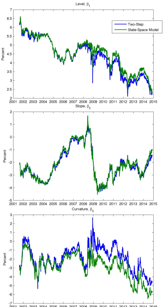
I have estimated the two-step DNS for the initial parameterization of the state-space
model, and it is worthwhile comparing the results obtained from both models to
understand how using a data dependent 𝜆 may improve the estimation. I have
included in annex the graphs that depict the evolution of the factor loadings estimated
by the one-step and two-step DNS with both the 20 and 30-years LLP.
Factors Mean Standard
Deviation Min Max 𝝆𝟑𝟎 𝝆𝟗𝟎 𝝆𝟏𝟖𝟎
Level 𝜷𝟏,𝒕 0.0458 0.0087 0.0240 0.0668 0.9227 0.8051 0.6823
Slope 𝜷𝟐,𝒕 -0.0241 0.0126 -0.0466 0.0152 0.9528 0.8206 0.6169
Curvature 𝜷𝟑,𝒕 -0.0228 0.0124 -0.0562 0.0013 0.8685 0.6649 0.4323
Decay Parameter 𝝀𝒕 0.4268
Factors Mean Standard
Deviation Min Max 𝝆𝟑𝟎 𝝆𝟗𝟎 𝝆𝟏𝟖𝟎
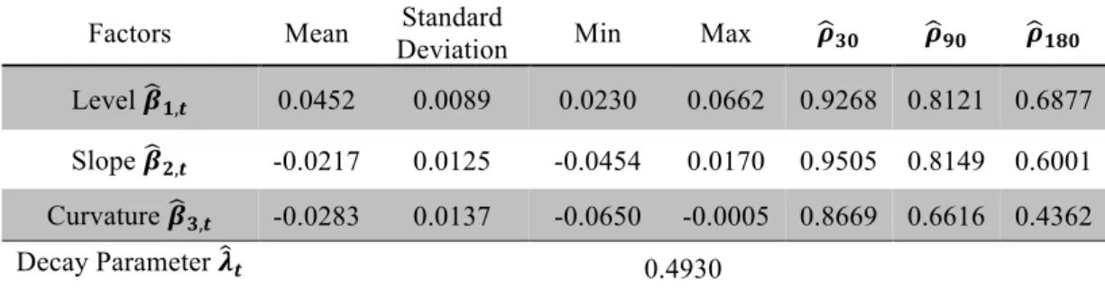
Level 𝜷𝟏,𝒕 0.0452 0.0089 0.0230 0.0662 0.9268 0.8121 0.6877
Slope 𝜷𝟐,𝒕 -0.0217 0.0125 -0.0454 0.0170 0.9505 0.8149 0.6001
Curvature 𝜷𝟑,𝒕 -0.0283 0.0137 -0.0650 -0.0005 0.8669 0.6616 0.4362
Decay Parameter 𝝀𝒕 0.4930
It seems that the one-step estimation is much more controlled in high volatility times
– as was the case in 2008 – but for the most part both estimation methods are quite
comparable. As expected the long-term factor, the level loading, is decreasing over
time. And if we look back at figure 3, it is possible to see how the 1-year rate (the
shortest maturity depicted) resembles the slope loading, which portrays the short-term
Table 2: Descriptive statistics of the DNS estimated parameters (level, slope and curvature) as well as the estimated decay rate for an LLP of 20 years.
factor in the DNS. The most puzzling is again the curvature loading – graphically the
estimation differs substantially using a different LLP. In particular the estimation
using a longer LLP is more volatile, which is especially noticeable around 2008/2009
at the time of the financial crisis.
4.3 Smith-Wilson parameters
Once again the estimation of the Smith-Wilson parameters was done for both an LLP
of 20 and 30 years. In this case the estimated parameters z do not have any economic
interpretation as in the DNS as the model estimates parameters for each maturity that
best fit that data point. This was also the reasoning behind proposing that this method
would provide a better fit in-sample than the DNS. Taking this into account I will
include the descriptive statistics for these parameters in annex just for reference but
will not discuss them. Instead I will analyze the Smith-Wilson estimation in the next
sub-section.
4.4 Estimated and extrapolated yields
Now I will present the yield curves resulting from the application of the calibrated
models, including their extrapolation beyond the 20 or 30-years last liquid point and
up to a maximum maturity of 100 years.
This analysis can be split into two: the in-sample fit (from maturities 1 to 20/30 years)
and the out-of-sample fit (from maturities 21/31 to 100 years). Starting with the in
sample fit it can be seen in figures 4 and 5 the average yield curve fitted using the
Smith-Wilson and DNS models. The discrepancy when using 30 years of observable
data becomes noticeable in the case of the DNS, which constructs a smooth curve by
calibrating the parameters taking into account the entire data sample. Note also how it
is a result of the model’s nature as it has been mentioned before, where the
parameters’ job is to achieve the best fit to the observable data and do not carry any
economic meaning like in the DNS.
To quantify this deviation I have computed the RMSE for the in-sample maturities.
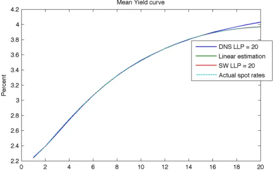
Figure 4: Mean yield curve fitted by the DNS and SW using an LLP of 20 years versus the actual spot rates and a linear interpolation method.
estimation deviates more from the actual spot rates than the SW estimation and that
this difference worsens at the short and long ends of the curve. In the graphs provided
in annex it is also possible to see that in distressed times, such as the day in which
Lehman Brothers’ filled for bankruptcy, the discrepancy between the market rates and
the DNS estimation is bigger. It should also be noted that the yield curve on this
particular day has a shape far from what would be considered a typical yield curve.
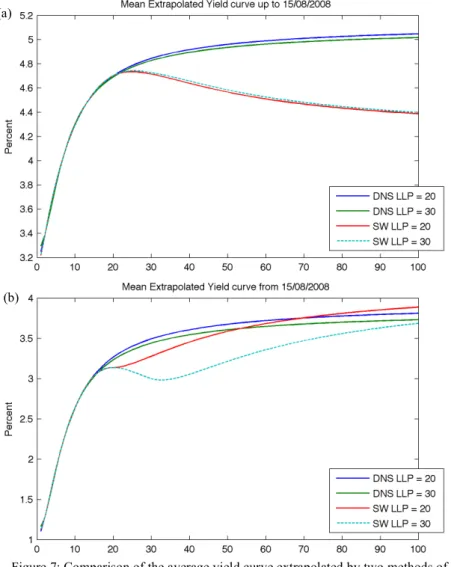
When it comes to extrapolation beyond the last liquid point, the graphical results of
the average extrapolated yield curve can be seen in figure 6 and the descriptive
statistics of the extrapolated rates will be included in annex.
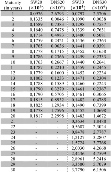
Maturity (in years)
SW20
(×𝟏𝟎𝟒)
DNS20
(×𝟏𝟎𝟒)
SW30
(×𝟏𝟎𝟒)
DNS30 (×𝟏𝟎𝟒) 1 0,0976 2,6793 0,0797 2,5706 2 0,1335 0,0046 0,1090 0,0038 3 0,1589 0,7383 0,1298 0,7537 4 0,1640 0,7478 0,1339 0,7631 5 0,1714 0,4983 0,1400 0,5081 6 0,1759 0,2421 0,1436 0,2363 7 0,1765 0,0636 0,1441 0,0391 8 0,1778 0,1715 0,1452 0,1658 9 0,1786 0,2366 0,1459 0,2333 10 0,1763 0,2667 0,1440 0,2641 11 0,1787 0,2210 0,1459 0,2445 12 0,1779 0,1600 0,1452 0,2234 13 0,1802 0,1233 0,1471 0,2304 14 0,1788 0,1589 0,1460 0,2243 15 0,1790 0,3279 0,1461 0,2367 16 0,1790 0,5705 0,1461 0,3065 17 0,1815 0,8932 0,1482 0,4785 18 0,1825 1,2934 0,1490 0,7399 19 0,1778 1,7596 0,1452 1,0698 20 0,1817 2,2998 0,1483 1,4672
21 - - 0,3634 1,8488
22 - - 0,5687 2,3024
23 - - 0,8478 2,7787
24 - - 1,2127 3,2807
25 - - 1,5724 3,7768
26 - - 2,0030 4,2668
27 - - 2,4436 4,7599
28 - - 2,8961 5,2416
29 - - 3,3500 5,7079
30 - - 3,7790 6,1506