www.nonlin-processes-geophys.net/15/25/2008/ © Author(s) 2008. This work is licensed
under a Creative Commons License.
in Geophysics
Sequence of eruptive events in the Vesuvio area recorded in
shallow-water Ionian Sea sediments
C. Taricco, S. Alessio, and G. Vivaldo
Dipartimento di Fisica Generale dell’Universit`a, V. Pietro Giuria 1, 10125 Torino, Italy and Istituto di Fisica dello Spazio Interplanetario (IFSI)-INAF, C. Fiume 4, 10133 Torino, Italy
Received: 30 July 2007 – Revised: 14 December 2007 – Accepted: 14 December 2007 – Published: 28 January 2008
Abstract. The dating of the cores we drilled from the Gal-lipoli terrace in the Gulf of Taranto (Ionian Sea), previously obtained by tephroanalysis, is checked by applying a method to objectively recognize volcanic events. This automatic sta-tistical procedure allows identifying pulse-like features in a series and evaluating quantitatively the confidence level at which the significant peaks are detected. We applied it to the 2000-years-long pyroxenes series of the GT89-3 core, on which the dating is based. The method confirms the dat-ing previously performed by detectdat-ing at a high confidence level the peaks originally used and indicates a few possible undocumented eruptions. Moreover, a spectral analysis, fo-cussed on the long-term variability of the pyroxenes series and performed by several advanced methods, reveals that the volcanic pulses are superimposed to a millennial trend and a 400 years oscillation.
1 Introduction
The study of climatic time series measured in marine sedi-ment cores allows reconstructing past natural variability. In order to reliably reveal both high and low frequency oscil-lations, long high-resolution time series are required (e.g., Martinson et al., 1995). Moreover, in these researches, an accurate dating guarantees the reliability of the measured cli-mate proxy records.
Over the last 20 years, the Torino cosmo-geophysics group has carried on researches based on the study of climatic time series measured in shallow-water sediment cores drilled from the Gallipoli terrace in the Gulf of Taranto (Ionian Sea). This is a particularly favorable site for high resolution climatic studies, due to a high sedimentation rate and to the possibil-ity of accurate dating, offered by presence along the cores of Correspondence to:C. Taricco
volcanic markers, related to eruptive events occurred in Cam-panian area, a region for which an accurate documentation of the major eruptions is available, starting from the Pom-pei plinian event (79 AD). Historical documents are quite de-tailed for the last 350 years (a complete catalogue of eruptive events, starting from 1638, is given by Arn`o et al. (1987)), while they are rather sparse before that date.
The absolute dating of several cores retrieved from the Gallipoli Terrace, at a water depth of about 200 m (Cini Castagnoli et al., 1990, 1992; Bonino et al., 1993; Cini Castagnoli et al., 1999, 2002), was obtained using radiomet-ric methods and tephroanalysis. The210Pb method
(Krish-naswamy et al., 1971), applied to the upper 20 cm of the cores, revealed that 1 cm of mud is deposited in about 15.5 years. In order to check the sedimentation rate determined by this method and its constancy with depth, the number density of pyroxene grains was measured along the cores. In the sed-iment layers expected on the basis of the210Pb dating, 22 sharp peaks were identified, that correspond to known vol-canic eruptions occurred in the Campanian area during the last two millennia. The linear time-depth relation turned out to beh=(0.0645±0.0002)yBT, wherehis depth in cm and
yBT means year-before-top (top=1979 AD), with a
correla-tion coefficientr=0.99. The slope of this line is the sedimen-tation rate, which remained constant over the last two millen-nia and across the whole Gallipoli Terrace (Cini Castagnoli et al., 1990, 1992; Bonino et al., 1993; Cini Castagnoli et al., 2002).
0 200 400 600 800 1000 1200 1400 1600 1800 2000 0
50 100 150 200 250
Time (years A.D.)
Pyroxenes number/0.5 mg
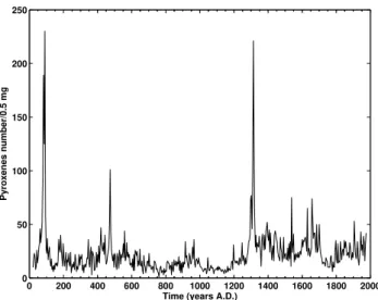
Fig. 1. Pyroxenes series measured in the GT-89-3 shallow-water Ionian core.
obtained by applying this method, useful to test our original dating approach.
2 The series
The pyroxene series measured in the GT89-3 core is shown in Fig. 1. This core was sampled every 2.5 mm, correspond-ing to a samplcorrespond-ing intervalTc=3.87 years; 506 samples were
measured, covering the interval from 20 to 1975 AD. In this series, two huge peaks, corresponding to the eruptions of Pompei (79 AD) and Ischia (1301 AD) are present; another smaller but still very pronounced peak marks the Pollena eruption (472 AD).
3 The method
The method for the automatic extraction of pulse-like sig-nals, applied here, was proposed by Naveau et al. (2003) (see also Naveau and Amman, 2005). The model originated from the need of solving modeling drawbacks, that emerged when analyzing time series resulting from the superposition of an irregular, abruptly changing pulsatile component and a slowly changing one. The approach has a general validity and can be applied to every series with these characteristics, such as a volcanic record.
From a statistical point of view, this procedure allows to accurately and objectively identify the timing of pulse-like events and to extract their intensities from the noisy and low-frequency components of the signal. The model also esti-mates the signal subsequent evolution and provides, by asso-ciating a posterior probability to each extracted spike, a con-fidence measure that allows focusing on those events which have been detected with high probability, while considering
the other ones as background noise. Unlike the classical threshold techniques, this method takes into account the time variability of the noisy component of the series and uses the local characteristics of the signal to associate to each pulse a probability which is not necessarily linked to the absolute intensity of the spike.
The time series is split into three main components, as-sumed to be mutually independent: y(t )=x(t )+f (t )+ǫ(t ), wherey(t )is the observed time series, x(t )is the abruptly changing component (in our case the pulsatile volcanic sig-nal),f (t )is the baseline (i.e. the slowly changing component representing the long-term trend and possible low-frequency components) and ǫ(t ) indicates Gaussian white noise with zero mean and standard deviationσǫ.
The volcanic signalx(t )is modeled by a multi-process dy-namic linear model. The parameters estimation for this kind of models becomes more and more complicated at the grow-ing of the number of compartments which are dealt with. The one-compartmental model, represented by an exponen-tial decay (Kushler and Brown, 1991), thus turns out to be the easiest one for deriving the system transfer function: the signalx(t )is represented by an exponential-decay-towards-baseline model, which decomposes it into a pulsatile vol-canic inputv(t )convoluted with an exponential decay, that expresses the damping with time of the eruption effect.
For series sampled at constant rate, the exponential decay reduces to a first-order autoregressive process AR(1), so that x(t )is represented by x(t )=ax(t−1)+v(t ), wherea (with
|a|<1) is a constant representing the exponential decay and v(t )is a random variable modeling the strength of the erup-tion:v(t )=N (µx, σx2)ifo(t )=1 andv(t )=0 ifo(t )=0. Here
o(t )is a binary Bernoulli random variable, whose parameter π=P[o(t )=1]denotes the a priori probability of observing an eruption at time t. So ifo(t )=1 (eruption), the volcanic input is equal to a random normal variable with meanµxand
varianceσx2; ifo(t )=0 (no eruption),v(t )is zero.
As it is well known, the general definition of multi-process dynamic linear models is based on the idea that it exists a finite number of underlying processes and that an observa-tional mechanism allows us to observe only one of them at each time; in our case, the pyroxenes time series pulsatile component is simply represented by two latent processes, re-spectively having and not having an eruption (a pulse) at a given timet.
elements depending on the smoothness parameterλ, which controls the smoothness of the curve. Thus, the perturbation is modeled as a random effect representing the smoothing de-viation of the overall fitted curve from the straight line. The most commonly used form for the polynomial spline, i.e. the cubic spline (corresponding to m=2), is then adopted in the model.
The slowly and the abruptly changing components present in the series require a simultaneous estimation. Assuming an additive structure in the state-space frame, all the pre-vious models are then embedded into a unified state-space model (SSM) belonging to the large class of Multi-Process State-Space Models, which is employed for the coinciden-tal estimation of both the series components (the volcanic pulses and the background trend) and the associated noise, thus overcoming the previously mentioned modeling draw-backs. The state-space representation (also known astime domain approach) provides a convenient and compact way to model and analyze systems with multiple inputs and out-puts. Unlike the frequency domain approach, this kind of representation is not limited to systems with linear compo-nents and zero initial conditions.
Let us recall that the basic idea of a state-space model is that a dynamic system is not directly observable without er-rors, so that the observations of a system state consist of a latent state (state vector) and a multiplicative or an additive random error. The structure of the system is fully described by the state vector, which in general contains the unknown parameters that are to be determined (structural parameters) and other parameters controlling the structure of the system. In particular, the observed time seriesy(t ) is generated by two structural equations:
– theobservation-level equation, a matrix representation fory(t ), which is now defined as a linear combination of the state vector representing the various unobserved (or latent) components of the system and an additive, normally distributed random error. This first equation gives an idea of how the different forcings can influence the observations;
– the system-level equation, a simultaneous matrix rep-resentation of both the latent processesx(t ) andf (t ), modeling the forcings temporal dynamics. More gener-ally, this is a Markov transition equation, which speci-fies the latent processes structure by describing the state vector time-evolution, and gives a clear interpretation of the structural parameters.
The Multi-Process State Space Model is preferable to other approaches from a statistical point of view, since it re-duces errors propagation and, thanks to its hidden Marko-vian structure, it allows to adopt existing efficient estimation procedures, such as the Multi-process Kalman Filter (MKF) (Harrison and Stevens, 1971, 1976). This recursive forward algorithm, characterized by one-step-ahead prediction and
filtering steps, allows the evaluation of the state vector poste-rior probability and of an approximate likelihood function, which is maximized to produce maximum likelihood esti-mates for the unknown parameters (Guo and Brown, 2000). MKF is an extension of the most common Kalman filter (ap-plied to Gaussian state-space models) used when the assump-tion of normality breaks down, i.e. when the state vector fol-lows a mixture of distributions, as in the case of the pulsatile component of our pyroxenes series. Notice that the essen-tial difference between Kalman filtering and a conventional linear model is that the state vector is not assumed to be con-stant, but it may change in time according to a system of differential equations.
Following the work by Guo et al. (1999), who put for-ward the use of this method in the biological and medical field, Naveau et al. (2003) apply an extended MKS approach to obtain the volcanic inputv(t )posterior probability from the state-vector estimate, by augmenting v(t )into the sys-tem state vector. At each time step, four model outputs are calculated:
– f (t )= baseline (long-term trend) – v(t )= volcanic input
– x(t )= volcanic signal
– p(t )=a posterioriprobability of an eruption
In the present work, we have applied the original Gaus-sian peak-amplitude-distribution model (Naveau et al., 2003; Guo et al., 1999). The outputs have been computed using the software freely made available at http://www.cceb.upenn. edu/pages/wguo/.
An underlying assumption of the model is that the mag-nitudes of the extracted volcanic pulses follow a Gaussian distribution, while only the largest events usually leave a clear and distinct signature in the sediments, so that the vol-canic spike amplitudes follow a heavy skewed distribution rather than a Gaussian one, taking values outside the Gaus-sian tail. Since the model assumption of pulses homogene-ity thus breaks-down for the two dominant peaks in the py-roxenes time series (Pompei and Ischia), we have performed the analysis excluding these two amplitude extremes, by di-viding the series into two parts: 150–1250 AD and 1350– 1975 AD.
In order to be able to model also the largest volcanic erup-tions, the statistical distribution followed by the volcanic pulses magnitudes should be asymptotically approximated by a Generalized Pareto Distribution (GPD), which is able to fit extremes from any continuous distribution and not only from a Gaussian sample (Naveau and Amman, 2005).
(SSA), Multi-Taper Method (MTM) and Wavelet Transform (WT).
The SSA technique was designed to extract information from short and relatively noisy time series, such as climatic ones. It provides data-adaptive filters that separate the time series into components that are statistically independent and can be classified as trends, oscillatory patterns and noise. The trends need not be linear and the oscillations can be ampli-tude and phase modulated. SSA has been applied to many instrumental and proxy climate records (e.g., Ghil and Vau-tard, 1991; Plaut et al., 1995; Cini Castagnoli et al., 2002); two review papers (Ghil and Taricco, 1997; Ghil et al., 2002) and references therein cover both methodology and other ap-plications. Significant variability components may be recon-structed by this method (Ghil and Vautard, 1991; Ghil and Taricco, 1997; Ghil et al., 2002). For the calculations we have used the freeware SSA-MTM Toolkit (Vautard et al., 1992) at http://www.atmos.ucla.edu/tcd/ssa/.
The MTM (e.g., Ghil and Yiou, 1996; Ghil and Taricco, 1997; Ghil et al., 2002) is a high-resolution spectral method by which significant oscillatory components in a series can be singled out, both assuming a red noise background and a background of locally white noise (i.e. a colored noise pro-cess that varies slowly but arbitrarily with frequency: a hy-pothesis allowing for noise background with a complicated structure (Mann and Lees, 1996)), and then reconstructed.
The WT allows an evolutionary spectral analysis of a se-ries in the time-scale plane (e.g., Foufoula-Georgiou and Ku-mar, 1994; Percival and Walden, 2000). The concept of scale is typical of this method: the scale is a time duration that can be properly translated into a Fourier period, and hence a fre-quency. The Continuous Wavelet Transform (CWT) in spec-tral applications is discretized by computing it at all available time steps and on a dense set of scales (Torrence and Compo, 1998). The square modulus of the transform expresses spec-tral density as a function of time and frequency. A filtered version of the signal can then be reconstructed selecting only the contributions from a given set of frequencies. By time averaging the CWT at each value of frequency (scale), the Global Wavelet Spectrum (GWS) and the corresponding sig-nificance levels can be computed, using a background spec-trum of red noise, thus obtaining a time-averaged spectral es-timate comparable with those obtained by classical methods. However, CWT is a multiresolution analysis: frequency res-olution is high at low frequency and poor at high frequency (Torrence and Compo, 1998). It is therefore particularly suited for determining the frequency of oscillations in the low-frequency range of the spectrum and to reconstruct them accurately. The calculations have been performed according to the guidelines given in Torrence and Compo (1998).
The arbitrarily discretized CWT described above is redun-dant: the number of samples derived from CWT is much greater than the minimum that would be sufficient to ensure that all the information present in the original signal is re-tained, so that the signal can be reconstructed from the
trans-form values. In other words, CWT may be seen as an ex-pansion of the series in a non-orthogonal basis. The idea of critical sampling (retaining the minimum information nec-essary for signal reconstruction) and of an orthogonal basis leads to the Discrete Wavelet Tranform (DWT), that can be quickly computed through an efficient algorithm (pyramidal algorithm) developed by Mallat (1989). For computational reasons, the DWT is performed on series of lengthNequal to an integer powerJof 2:N=2J. The DWT allows an additive decomposition of a series into a low-frequency ”smooth” and a number of high-frequency “details” (Percival and Walden, 2000). More specifically, the series is expressed by the sum ofJ+1 details, where eachj-th detail (j=1, J+1) expresses the variations of the signal at larger and larger scales asj in-creases and the(J+1)-th one is equal to the sample mean of the observations. Let us now consider a particular level of decomposition j0. The sum of all the details of level
greater than j0 (i.e., from j0+1 to J+1) is defined as the
j0-th level smooth, and represents the cumulative sum of the
variations that are not expressed by thej0remaining details;
of course, it will be smoother and smoother asj0increases.
In other words, the fine scale features (high frequency oscil-lations) are captured mainly by the low-level detail compo-nents, while the coarse scale components (smooth and high-level details) correspond to lower frequency oscillations of the signal. This decomposition is known as MultiResolution Analysis (MRA).
Giving up orthogonality and thus returning to a certain degree of redundancy, the DWT scheme can be modified in order to gain interesting features that DWT does not posses. This approach is known under several names, as Non-Decimated Discrete Wavelet Transform or NWT (Na-son and Silverman, 1995) and Maximal Overlap Discrete Wavelet Transform or MODWT (Gencay et al., 2002). The MODWT can handle any sample size N; at each decomposi-tion level, the details and smooth coefficients of a MODWT MRA are N equally spaced samples as in the original se-ries, so that the temporal resolution at coarser scales is much better than with ordinary DWT; these coefficients are asso-ciated with zero-phase filters, so that events that feature in the original time series turn out to be properly aligned with features in the MRA; MODWT is invariant to circulary shift-ing the original time series (translation invariance) and thus avoids possible Gibbs-type phenomena and other artifacts in the reconstruction of a series that, on the contrary, can affect DWT. In the present work, we compared the low-frequency reconstructions obtained by CWT, SSA and MTM with the smooth obtained by MODWT, using Daubechies compactly supported wavelets (Gencay et al., 2002).
4 Results and discussion
0 200 400 600 800 1000 1200 1400 1600 1800 2000 0
10 20 30 40 50 60 70 80 90 100 110
Time (years A.D.)
Pyroxenes number/0.5 mg
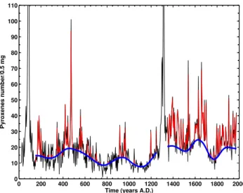
Fig. 2. Fit of statistical model (Naveau et al., 2003) to pyroxenes series. Thin black line: measured series; thin red line: model output
x(t )+f (t )(computed volcanic signal plus baseline, or long term trend); thick blue line: computed baselinef (t ).
as it can be seen in Fig. 2, in which the thin black line rep-resents the measured series, the thin red line is the model outputx(t )+f (t )(computed volcanic signal plus baseline, or long term trend) and the thick blue line is the computed baselinef (t ). The fit is particularly good in the more recent, post-1350 series section.
The computed baseline was then compared with the low-frequency components, determined applying the spectral methods mentioned before to the whole pyroxenes series.
Starting from SSA, we have adopted a window width of M=120, in order to be able to detect oscillations up to
≃500 y, while maintaining sufficient statistical significance. We have obtained, however, very similar results within a wide range of M values, ranging from 100 to 200 points. In the long-wave range the analysis has revealed a trend, rep-resented by the Empirical Orthogonal Function (EOF) 1 and accounting for∼9% of the total variance, and a∼400 y wave explaining∼14% of the total variance (EOFs 2,3). A Monte-Carlo model evaluation (Allen and Smith , 1996) performed with an ensemble size of 10000 reveals that these are sig-nificants components at 90% confidence level. They have therefore been reconstructed and their sum compared with the baseline, as shown in Fig. 3 (see the red and the blue lines, respectively).
The MTM reveals a trend and a component with period of
∼360 y, significant at 99% confidence level both assuming a background of red noise and of locally white noise (Mann and Lees, 1996). The corresponding reconstructed signal is also shown in Fig. 3, as a magenta-colored line.
The CWT analysis has been performed by a complex Mor-let waveMor-let with parameterω0=6. The GWS (not shown)
re-veals the presence of highly significant low-frequency
contri-0 200 400 600 800 1000 1200 1400 1600 1800 2000 0
10 20 30 40 50 60 70 80 90 100 110
Time A.D. (years)
Pyroxenes number/0.5 mg
Fig. 3. Comparison among baseline computed from the statis-tical model of Naveau et al. (2003) (thick blue line) and recon-structed low-frequency components of the pyroxenes series. Re-constructions according to Singular Spectrum Analysis (thick red line), Multi Taper Method (thick magenta line), Continuous Wavelet Transform (thick green line) and Non-Decimated Wavelet Trans-form (thick black line). See text for details. Also shown is the original series (thin grey line).
butions to the series variance, particularly at Fourier periods greater than∼1260 y (long-term trend) and around 400 y, in agreement with the results obtained by SSA and MTM. The corresponding reconstruction, performed by Inverse Contin-uous Wavelet Transform, appears in Fig. 3 as a green line.
At last, a MODWT decomposition of the pyroxenes sig-nal has also been performed, adopting a least asymmet-ric Daubechies wavelet LA(8). The level of decomposition J0=5 was chosen, since its smooth part contains, as in the
other cases, the low-frequency variability of the series up to
∼(400 y)−1. This smooth component is shown in Fig. 3, as a black line.
The baseline and the low-frequency spectral components reconstructed by four different methods are in phase agree-ment over the last two millennia, with the only exception of the most recent two hundred years. The differences among the amplitudes of the oscillations revealed by SSA, MTM CWT and MODWT, that may be noticed especially in the last centuries, may be due to the difficulty of these methods to handle a series that presents three sudden and strong peaks. Moreover, these low-frequency spectral components show greater amplitudes than the baseline, because these methods were applied to the complete pyroxenes series, including the two peaks of Pompei and Ischia, while the baseline was cal-culated excluding these two peaks.
1650 1700 1750 1800 1850 1900 1950 0
10 20 30 40 50 60 70 80
Pyroxenes number/0.5 mg
1650 1700 1750 1800 1850 1900 1950
0 0.5 1
Time (years A.D.)
Probability
Fig. 4. Results of automatic pulse-like peaks extraction from the pyroxenes series, for the post-1638 time interval documented in the catalogue by Arn`o et al. (1987). Upper panel: model output (thin green line) with segments, highlighted in red, corresponding to detected events. Black open circles and plus signs: historical dates of eruptions, ending Vesuvio activity cycles, used for the orig-inal tephroanalysis-based dating and corresponding dates calculated from the linear time-depth relation, respectively. Blue arrow: extra-eruption detected, documented in the catalogue but internal to an activity cycle. Lower panel:a posterioriprobability of an eruption. Thick red bars mark the dates at which probability attains 99%.
features is clearly revealed. In the next paragraphs, we ex-amine these events using theira posterioriprobability calcu-lated by the automatic extraction method described in Sect. 3. 4.1 Vesuvio activitypost-1638 AD
The catalogue by Arn`o et al. (1987) divides the recent Vesu-vio activity in cycles of widely variable length, separated by intervals of repose which also have variable duration. Each cycle ends with an eruption of moderate to violent explo-sive activity and may also include some intermediate erup-tive events. The last reported activity cycle ends with the 1944 AD eruption.
Figure 4 illustrates the results of the pulse-like features extraction for the time intervalpost-1638. The upper panel shows, as a thin green line, the model outputx(t )+f (t )(the same quantity plotted in Fig. 2), while the lower panel shows p(t ), thea posterioriprobability of a particular peak being recognized as an eruption, i.e., having the required pulse-like characteristics (thin green line). The thick red bars in the lower panel mark the dates at which p(t ) attains 99%; in the upper panel, the corresponding parts of the model out-put are highlighted in red. We prefer to use a high probabil-ity threshold (99%) because we analyzed the series without the 2 huge peaks of Pompei and Ischia; in this way we try to avoid an overestimation of the significance of the other
0 200 400 600 800 1000 1200 1400 1600 0
10 20 30 40 50 60 70 80 90 100 110
Pyroxenes number/0.5 mg
0 200 400 600 800 1000 1200 1400 1600 0
0.5 1
Time A.D. (years)
Probability
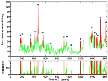
Fig. 5. Results of automatic pulse-like peaks extraction from the pyroxenes series for theante-1638 interval. Upper panel: model output (thin green line) with segments, highlighted in red, corre-sponding to detected events. Open circles and plus signs: historical dates of eruptions used for the original tephroanalysis-based dat-ing and corresponddat-ing dates calculated from the linear time-depth relation, respectively. Black signs for events detected at 99% prob-ability, blue signs for lower probability values. Cyan diamonds: possible undocumented detected events. Lower panel:a posteriori
probability of an eruption. Thick red bars mark the dates at which probability attains 99%.
peaks. The black open circles that appear near the peaks in the upper panel indicate the historical date of an eruption used for the original tephroanalysis-based dating. They are evidently in good agreement with the corresponding dates calculated from the linear time-depth relation given in the In-troduction (black plus signs in the figure). As it can be seen in Fig. 4, the model, with a probability threshold of 99%, recognizes all the 7 catalogue-documented events that we used for the tephroanalysis-based dating. All these events are eruptions ending a cycle of the Vesuvio activity. One extra-eruption, documented in the catalogue but internal to a cycle (1810 AD), is also detected (see blue arrow in the figure). 4.2 Vesuvio activityante-1638
90% probability and the remaining 2 historical events are de-tected at a lower significance level (<0.5). Moreover, the automatic extraction procedure reveals four possible events (cyan diamonds) that, to our knowledge, are not documented (346 AD, 914 AD, 1388 AD, 1472 AD).
This method has therefore led us to identifying in a more rigorous way the sequence of volcanic events useful for the dating of the sediment cores from the Gallipoli terrace. From a different point of view, the pyroxenes series is a good test for the method, since the detected peaks are supported by the historical documentation.
5 Conclusions
We have applied to the pyroxenes series measured in the shallow-water sediment core GT89-3 an automatic proce-dure that has allowed recognizing objectively as pulse-like volcanic events, at a high confidence level, the post-1638 peaks corresponding to the catalogue-documented eruptions we originally used to determine the sedimentation rate. The majority of the historical events in theante-1638 interval has also been recognized at high confidence level, thus confirm-ing the validity of the datconfirm-ing previously performed for the Gallipoli terrace. Moreover, a few possibleante-1638 un-documented eruptions have been identified.
Acknowledgements. We dedicate this paper to the memory of G. Cini Castagnoli and of G. Bonino, who many years ago started the study and performed the dating of the Gallipoli terrace. We are grateful to A. Romero for his dedicated technical assistance. This work was supported by the EC Project “Extreme Events: Causes and consequences” (E2-C2), Contract No 12975 (NEST).
Edited by: P. Yiou
Revieweed by: one anonymous referee
References
Allen, M. R. and Smith, L. A.: Monte Carlo SSA: detecting oscilla-tions in the presence of coloured noise, J. Climate, 9, 3373–3404, 1996.
Arn`o, V., Principe, C., Rosi, M., Santacroce, R., Sbrana, A., and Sheridan, M. F.: Eruptive History, in: Somma-Vesuvius, Quaderni de La Ricerca Scientifica, edited by Santacroce R., CNR, Roma, Italy, 114(8), 53–103, 1987.
Bonino, G., Cini Castagnoli, G., Callegari, E., and Zhu, G. M.: Ra-diometric and tephroanalysis dating of recent Ionian sea cores, Nuovo Cimento C, 16, 155–161, 1993.
Cini Castagnoli, G., Bonino, G., Caprioglio, F., Provenzale, A., Se-rio, M., and Zhu, G. M.: The carbonate profile of two recent Ionian sea cores: evidence that the sedimentation rate is con-stant over the last millennia, Geophys. Res. Lett., 17, 1937–1940, 1990.
Cini Castagnoli, G., Bonino, G., Provenzale, A., Serio, M., and Cal-legari, E.: TheCaCO3 profiles of deep and shallow
Mediter-ranean sea cores as indicators of past solar-terrestrial relation-ship, Nuovo Cimento C, 15, 547–563, 1992.
Cini Castagnoli, G., Bonino, G., Della Monica, P., Taricco, C., and Bernasconi, S. M.: Solar activity in the last millennium recorded in theδ18Oprofile of planktonic foraminifera of a shallow water Ionian Sea core, Solar Physics, 188(1), 191–202, 1999. Cini Castagnoli, G., Bonino, G., and Taricco, C.: Long term
solar-terrestrial records from sediments: carbon isotopes in plank-tonic foraminifera during the last millennium, Adv. Space Res., 29(10), 1537–1549, 2002.
Foufoula-Georgiou, E. and Kumar, P. (Eds.): Wavelets in Geo-physics, Academic Press, San Diego, California, 1994.
Gencay, R., Selcuk, S., and Whitcher, B.: An Introduction to Wavelets and other Filtering Methods in Finance and Economics, Academic Press, San Diego, California, 2002.
Ghil, M. and Vautard, R.: Interdecadal oscillations and the warming trend in global temperature time series, Nature, 350(6316), 324– 327, 1991.
Ghil, M. and Taricco, C.: Advanced spectral analysis methods, in: Past and Present Variability of the Solar-terrestrial System: Mea-surement, Data Analysis and Theoretical Models, edited by: Cini Castagnoli, G. and Provenzale, A., IOS Press, Amsterdam, The Netherlands, 137–159, 1997.
Ghil, M. and Yiou, P. : Spectral methods: What they can and can-not do for climatic time series, in: Decadal Climate Variability: Dynamics and Predictability, edited by: Anderson, D. and Wille-brand, J., Elsevier, Amsterdam, 139, 445–482, 1996.
Ghil, M., Allen, M. R., Dettinger, M. D., Ide, K., Kondrashov, D., Mann, M. E., Robertson, A. W., Saunders, A., Tian, Y., Varadi, F., and Yiou, P.: Advanced spectral methods for climatic time series, Rev. Geophys, 40(1), 3.1–3.41, 2002.
Guo, W., Wang, Y., and Brown, M. B.: A Signal Extraction Ap-proach to Modeling Hormone Time Series with Pulses and a Changing Baseline, J. Am. Stat. Assoc., 94(447), 746–756, 1999. Guo, W. and Brown, M. B.: Structural time series models with
feed-back mechanisms, Biometrics, 56(3),686–691, 2000.
Harrison, P. J. and Stevens C. F.: A Bayesian approach to short-term forecasting, Op. Res. Quart., 22, 341–362, 1971.
Harrison, P. J. and Stevens C. F.: Bayesian forecasting, J. Royal Stat. Soc. Ser B, 38, 205–247, 1976.
Krishnaswamy, S., Lal, D., Martin, J., and Meybeck, M.: Geochronology of lake sediments, Earth Planet. Sci. Lett., 11, 407–414, 1971.
Kushler, R. and Brown, M. B.: A model for the identification of hormone pulses, Statistic in Medicine, 10, 329–340, 1991. Mallat, S.: A theory for multiresolution signal decomposition: The
wavelet representation, IEEE T. Pattern Anal., 11, 674–693, 1989.
Mann, M. E. and Lees, J. M.: Robust estimation of background noise and signal detection in climatic time series, Climatic Change, 33, 409–445, 1996.
Martinson, D. G., Bryan, K., Ghil, M., Hall, M. M., Karl, T. R., Sarachik, E. S., Sorooshian, S., and Talley, L. D. (Eds.): Na-tional Research Council, Natural Climate Variability on Decade-to-Century Time Scales, National Academy Press, Washington D.C., USA, 1995.
Naveau, P., Amman, C., Oh H. S., and Guo, W. : An automatic sta-tistical methodology to extract pulse like forcing factors in cli-matic time series, in: Volcanism and the Earth’s Atmosphere, Geophys. Monogr. Ser., edited by: Robock, A., AGU, Washing-ton, D. C., USA, 139, 177–186, 2003.
Naveau, P. and Amman, C.: Statistical distributions of ice core sul-fate from climatically relevant volcanic eruptions, Geophys. Res. Lett., 32, L05711, doi:10.1029/2004GL021732, 2005.
Percival, D. B. and Walden, A. T.: Wavelet methods for time series analysis, Cambridge University Press, Cambridge, UK, 2000. Plaut, G., Ghil, M., and Vautard, R.: Interannual and interdecadal
variability in 335 y of Central England temperatures, Science, 268(5211), 710–713, 1995.
Torrence, C. and Compo, G. P.: A Practical Guide to Wavelet Anal-ysis, B. Am. Meteorol. Soc., 79, 61–78, 1998.
Vautard, R., Yiou, P., and Ghil, M.: Singular-Spectrum Analysis: A Toolkit for short, noisy chaotic signals, Physica D, 58, 95–126, 1992.
Wahba, G.: Improper priors, spline smoothing and the problem of guarding against model errors in regression, J. Royal Stat. Soc. Ser B, 40, 364–372, 1978.