EVALUATING THE PERFORMANCE OF AN AGV FLEET IN AN FMS UNDER MINIMIZING PART MOVEMENT AND BALANCING WORKLOAD RULES

(1)

School of Economics and Management TECNICAL UNIVERSITY OF LISBON

EVALUATING THE PERFORMANCE OF AN AGV FLEET IN AN FMS UNDER MINIMIZING PART MOVEMENT AND BALANCING

WORKLOAD RULES

Alberto Ferreira Pereira

ISEG - lnstituto Superior de Economia e Gestao

Abstract

The performance of an FMS with respect to AGV utilization is assessed using a simulation model. AGV fleets of different sizes are evaluated. Under OOM, an assignment rule designed to decrease time in system by minimizing part movements among machine tools, AGV utilization is lower than under WINO, an assignment rule that seeks to balance machine workload. For a given AGV fleet, machine utilization imbalance is more levelled under WINO than OOM, however comparing across the three AGV fleets, the maximum machine imbalance is smoother under OOM than under WINO. AGV utilization consistently decreases as the number of AGVs increases from eight to nine and then to 10. The system performance is adversely affected not only by too many AGVs but also by surplus spots in both inbound and outbound queues placed in front of the machine tools.

Keywords: AGV; AGV utilization; FMS; simulation.

Correspondence Address: Alberto Ferreira Pereira - ISEG, Rua Miguel Lupi n° 20, 1240-078 Lisboa. Email: albper@iseg.utl.pt .

(2)

PORTUGUESE JOUR/)/AL OF MANAGEMENT STUDIES, VOL. XVI, NO.2, 2011

INTRODUCTION

Growing competition in many industries has resulted in a greater emphasis on developing and using automated manufacturing systems which have quick response times and high flexibility (Chan, 2002). A flexible manufacturing system (FMS) consists of several numerically controlled workstations that can machine a wide variety of part types. Parts are mounted on the pallets, and automatic transportation devices are employed to transport them (Sarma et at., 2002). In an FMS, the automated guided vehicle system (AGV) is an excellent choice for material handling because of its automation of loading and unloading, flexibility in path movement, ease of modification of the guide-path network and computer control (Um et at., 2009). AGVs possess more flexibility and capacity than other conventional material handling systems, especially for the FMS (Yeh and Yeh, 1998).

Measurements of the performance of an AGV system include AGV utilization, throughput, and a load's average time in system (Bischak and Stevens, 1995).

The main purpose of this research is to evaluate the performance of a dedicated FMS with respect to AGV utilization (U). Two rules to assign machines to parts, three rules to sequence jobs at a particular machine, three levels of available AGVs, and two levels of machine commonality will be tested. The performance will be evaluated across the ensuing 36 different configurations (36=2x3x3x2).

Parts will be loaded onto a pallet in accordance with the first-come-first-served discipline. Once loaded, there is a need to assign the part to the machine-tool (MT) required to perform the next operation. The assignment decision will be based upon one of the two assignment rules (A): OOM (Only One Machine) and WINQ (Work IN Queue). Following the machine assignment decision, parts will be launched into the FMS and scheduled in front of the MT to be processed on the basis of one of three sequencing rules (S): shortest processing time (SPT), SPT divided by total processing time (SPT/TOT), and most operations per part (MOPP). Because the performance of an FMS has been shown to be related to the configuration and hardware available to move parts around the system, the number of AGVs (V) will be defined as the third experimental factor and it will be set at three different levels of intensity: three, five and seven AGVs. Finally, the number of parts that can be entirely processed on one single machine, machine commonality (M), is set at two levels: at the high level, seven parts out of a total of 10 can be entirely processed on one single machine, whereas at the low level only three out of 10 parts can be entirely processed on one single machine.

LITERATURE REVIEW

Automated guided vehicles are increasingly being used for material transfer in production lines of modern manufacturing plants. The purpose is to enhance efficiency in material transfer and increase production (Singh et at., 2011 ).

Shang and Sueyoshi (1995) developed a structured framework to support management's deliberation on issues of FMS design and planning which is specifically

(3)

PORTUGUESE JOURNAL OF MANAGEMENT STUDIES, VOL. XVI, NO. 2, 2011 intended to assist managers in selecting the most appropriate FMS design. Um eta/.

(2009) simulated a hypothetical FMS comprised of six machine centres, an AGV system with a fixed guide-path and incoming and outgoing conveyors. AGV utilization was one of the critical factors in the experiment and was defined as the percentage of total simulation time that vehicles spent delivering and retrieving parts. Singh et a/. (2011) addressed the problem of scheduling of AGVs for efficient and uniform material distribution and used AGV utilization as one performance measure.

Reddy and Rao (2006) developed a hybrid genetic algorithm to address the combined machine and vehicle-scheduling problem to generate an optimum machine and vehicle schedule that is best with respect to the makespan, mean flow time and mean tardiness. Iwata eta/. (1982) provided a heuristic approach, using a decision rule to obtain a good feasible solution for a practical large-scale problem. Three proposed decision rules were investigated through a case study with respect to makespan, mean flow time, mean utilization of machine tools, and mean utilization of transport devices. Shanker and Tzen (1985) simulated an FMS to compare the solutions of loading given by mixed integer programming and heuristics methods with respect to CPU time, unbalance and number of tool slots used, and to investigate the effect of loading policies in conjunction with fout dispatching rules on system performance as measured by machine utilization. Ozden (1988) conducted a simulation study of multiple-load-carrying AGV in an FMS whose performance was measured with respect to throughput, average utilization of the machining station, and average utilization of the AGVs. Kuzgunkaya and EIMaraghy (2007) present a fuzzy multi-objective mixed integer optimization model to evaluate reconfigurable manufacturing system investments used in a multiple product demand environment and compare the performance of flexible and reconfigurable systems.

EXPERIMENTAL FACTORS

ASSIGNMENT RULES

OOM attempts to assign to each incoming part a machine that can perform all the operations required by the part. If this machine is not available at the time it is needed or if such a machine does not exist, OOM then attempts to assign a machine that can complete the next largest number of consecutive operations required by the part. This process continues until a machine that can process at least one operation is found. In the event that more than one machine is found to be available, OOM randomly selects the machine to assign to the part. If no machine is found to be available, the incoming part is routed to a parking area where it waits until any machine becomes available.

The WINO rule assigns machines to incoming parts on the basis of the current total processing time allocated to the parts located in the queue preceding the machine. A part requesting processing for a particular operation will cause WINO to scan the machines for one capable of performing the requested operation with at least one spot available in its input queue. Those meeting this requirement are placed in a temporary

(4)

PORTUGUESE JOURNAL OF MANAGEMENT STUDIES, VOL. XVI, NO.2, 2011

candidate machine set. If two or more machines are placed in the set, WINO assigns the machine with the current lowest total processing time requirement reflected in its input queue. If no candidate machine can be selected, WINO parks the part requesting processing in a waiting area until any machine becomes available.

SEQUENCING RULES

SPT orders parts to be processed in front of the MT according to the shortest operation time first. SPT/TOT rule orders first the part with the shortest processing time for the operation divided by the total processing time for the part. MOPP orders the part with the highest number of consecutive operations that can be processed in an MT first. In the event of a tie between parts, the part with the largest total processing time is scheduled first.

NUMBER OF AGVS

Fleets of three, five and seven automated guided vehicles will be tested.

MACHINE COMMONALITY

Machine commonality defines the number of parts that can be completely processed on one single machine. The system is composed of five identical numerically controlled machines, but each machine is capable of processing only certain parts based on the tools assigned to its tool magazine. Seven of the ten parts could be entirely manufactured on one machine. The notion that a large fraction of the part types can be made on a single machine is consistent with the goals of current FMS loading and tool assignment research (Shanker and Tzen, 1985). Since it is possible that a large number of "one machine" parts might grant the OOM assignment rule an unrealistic advantage, this study also defines one other level where only three parts can be processed on one single machine. Hence, two levels - high and low - will be defined for this experimental factor. At the high level, seven parts out of a total of ten can be entirely processed on one single machine. At the low level, only three out of ten parts can be processed on one single machine.

THE MANUFACTURING SETTING

In the FMS we simulated, parts are handled by automated guided vehicles. An FMS consists of a numerically controlled (NC) machine, a material handling system (MHS} and a computer control system for integrating the NC machine and the MHS.

(5)

The integration of these machines and facilities generally involves the use of a controller, complex software and an overall computer control network that coordinates the machine tools (MT), the material handling, and the parts (Um eta/., 2009).

The FMS produces ten parts on five identical MTs. Each machine is able to process only certain part types on the basis of the tools that are available in that machine's tool magazine. A load/unload work centre is located beside the machine-tools area. The parts to be manufactured arrive at the system as raw work pieces. Part arrival is described by a uniform distribution. Upon arrival, parts are loaded onto pallets at the load/unload work centre. The loading takes place on a first-come-first-served basis as soon as a pallet becomes available in the load/unload station. The time to load a part onto a pallet is uniformly distributed between 0.75 and 1.0 minute.

Depending upon the part type, the required number of operations varies between two and four (Chen and Chung, 1996; Sridharan and Babu, 1998). Pallets holding parts to be manufactured are moved throughout the FMS by means of the AGV system. Each machine is preceded by an input queue. When the pallet arrives before the queue in front of the machine, a transfer mechanism is activated by the control computer and the pallet is shifted from the AGV onto the on-shuttle. The on-shuttle has the capability of rearranging work-parts for processing according to the sequencing priority. Work parts entering the queue preceding the machine-tools are placed ahead of previously .·· .·placed work parts wifh lower sequencing priority (Chang et at., 1986): The AGV is then released to cruise along the guided path until a new request is issued. If the MT is busy, the part requiring processing waits in the input queue until the machine becomes available.

Processing begins as soon as the MT becomes available. Once processed, the part is moved to the output queue following the MT to wait for a free transporter to collect and carry it to the next destination (MT or unload). If, when a machine finishes processing a part, there is no available space in the output queue to which the part can be moved, the machine is blocked and is unable to process the next part. Both the input and the output queues have a capacity of five work-parts and pallets (Choi and Malstrom, 1988; Sabuncuoglu and Hommertzheim, 1989).

Completed parts are removed from the pallet at the load/unload work centre before leaving the system. The pallet is then reloaded or stored until needed. The pallets are of the general purpose type and unrestricted, so that whenever a move request is sent to an AGV, a pallet is assumed to be available. Figure 1 depicts the dedicated FMS simulated in this study. The AGV system consists of a variable number of vehicles that move unidirectionally on one of two-railed tracks. One track accommodates forward movement, the other reverse. To change an AGV direction, a special mechanism activates the crossover links to shift the AGV from one track to the other. Bidirectional movement is allowed along the crossover links between the two main tracks. Sixteen control points are defined along the track. When an AGV reaches a control point, it may receive instructions regarding its movement (load, unload, proceed, or wait). During the operations of the system, idle vehicles cruise along the guided path until a

request is placed. '

(6)

84

FIGURE 1 The FMS

Load/Unload

TABLE I

Operations required to manufacture all parts

Operation

2 3 4 5 6 7 8 9

---~----

--·--·--·--·---··-·---Part

A(h, /) 1 2 6

B (h) 3 5 2

C (h, I) 2 2 1

D (h) 6 5 4

E (h, I) 2 8

F (h, /) 9 4

G (h) 5 4

H (h, I) 3 7

I (h) 3 5

J (h) 6 1

K (I) 3 5 2

L (/) 6 5 4

M (/) 5 4

N (/) 3 5

0 (/) 6

---·---·---Machine

2 3

4

5

(7)

---·---·--·-·--··-··---·-·-··---PORTUGUESE JOURNAL OF MANAGEMENT STUDIES, VOL. XVI, NO. 2, 2011 Two groups of 10 parts are defined. Seven out of the 10 parts of the first group can be entirely processed on one single machine, whereas in the second group only three can be entirely processed on one single machine. We call the first, high machine commonality group, and the second, low machine commonality group. The first group corresponds to the high level of machine commonality experimental factor, the second to the low level. A previous study (Gunther eta/., 1998) used commonality as an experimental factor set at two levels, high and low. An entry of 1 in the bottom portion of Table I indicates the operation in that column can be performed by the machine. The top portion shows the time (in minutes) to process the operations required by the part. For each part, operations are processed in the sequence shown,from left to right. Part name is followed by an indication to which group it belongs: high machine commonality (h), or low (1). Total processing time over both groups is the same.

It is felt that keeping the total processing time constant over the two groups and maintaining an equal number of parts are preferable to maintaining a fixed set of ten parts and changing the machine environment by altering the set of tools assigned to each machine loaded into the MT magazine. A change in tool assignment might significantly affect the relative operating characteristics of the five machines, thereby reducing our ability to compare results across the machine commonality factor setting. It is possible to route each part through the system in several different ways. A total of 120 and 131 different routings are possible for the high and low commonality product groups, respectively. The number of routings for any part p is:

9

n(Opj X Mj) j=l

where:

Opj is set equal to 1 if part p requires operation j, and set equal to 0 otherwise. Mj- is the number of machines that process operation j.

(1)

For example, for part E (p=E), using (1 ), the number of routings is found to be equal to eight. The complete enumeration of the routings for part E is shown in Table II. Table entries indicate all possible combinations to sequentially process operations four and six. Some of the routes are dominated by others and may be dropped from further consideration.

Operation

4

6

TABLE II

Routings for part E

Route

2 3 4 5

2 2 2 2 3

2 3 4 5 2

6

3

3 ---·---·

·-7 8

3 3

4 5

(8)

Routing one dominates routes two, three and four and routing six dominates routes five, seven and eight. Because of the dominance effect, the total of 120 and 131 rout-ings is reduced to 56 and 58, respectively. Input variables for this study and their as-sociated distributions and

parameters, presented in Table Ill, have been found in previous studies (Iwata eta/.,

1982; Shanker and Tzen, 1985; Sarin and Chen, 1987; Ozden, 1988; Chan, 2002).

TABLE Ill

Flexible manufacturing system operational data

---·---~---Number of identical machines 5 Time to un/load AGV 0.3 minutes

Number of parts 10 AGV (loaded) speed/min 75m

Average shop loading 70% AGV (empty) speed/min 18m

Number of pallets Disposition of idle AGVs Cruise

Number of AGVs 3,5, 7 Initial location of AGVs Variable

Parts inter-arrival time Uniform Number of control points 16

Input/output queue capacity 5 Number of segments 16

Using a uniform distribution for parts inter-arrival with mean of 2.857 minutes, this research seeks 70% average machine utilization over the simulation horizon, midway within the range from 52% to 88% reported in the literature (Shanker and Tzen, 1985; Denzler and Boe, 1987; Ozden, 1988). Time to load or unload an AGV is short as a result of automation. Descriptions of actual systems report load/unload cycle times as low as five seconds (Miller and Subrin, 1987). Sabuncuoglu and Hommertzheim (1989) used 0.3 minutes to load/unload the AGVs. Elsayed and Boucher ( 1985) have reported AGV speeds varying from 61 to 79 m/min.

Tools required for the entire sets of operations performed by any machine have been loaded onto the tool magazine of each MT. Machine-tools are assumed to work without breakdowns. The manufacturing environment to be studied is consistent with respect to the hardware specifications and operational parameters (Shanker and Tzen, 1985; Denzler and Boe, 1987; Ozden, 1988; Sabuncuoglu and Hommertzheim, 1989; Nance and Sargent, 2002). This study addresses the research hypotheses listed in Table IV.

THE SIMULATION MODEL

A simulation model is developed to address the research hypotheses. Visual SLAM® and AweSim® were used in the modelling of the FMS (Pritsker et at., 1997). AIDurgham and Barghash (2008) state the importance of simulation in manufacturing namely in the material handling arena. Simulation has also been used to study maintenance policies (Yun eta/., 2008) and to assist decision makers in the complex shipbuilding industry where traditional static planning and scheduling no longer provide sufficient results for controlling its complex and interwoven elements (lee et at., 2009).

(9)

PoRTUGUESE JOURNAL OF MANAGEMENT STUDIES, VOL. XVI, NO. 2, 2011 Dhouib et a!. (2009) used AweSim® and VisuaiSiam® to measure the effective throughput of non-homogeneous automatic transfer lines. Control statements to monitor the crossing of state variables against a threshold, servers, physical characteristics for the AGVs, the flow of entities through both regular and service activities, logic and decision nodes, and rules to stop the simulation and to collect statistical observations are defined. Subroutines are developed to access the attributes of the parts in the output queue following the MT to facilitate a decision to request a vehicle from the AGV fleet and to reroute the part to the next available machine to perform the next operation, or to request a vehicle to transport the part to the unloading area to exit the system. Parts created at the load/unload area according to a uniform distribution carry a set of 12 attributes to store part characteristics such as creation time, part type or number of required operations. Attribute value can be defined as a constant, it may vary as the part flows through the network, or it may be set as binary (0-1) to define a mutually exclusive condition.

Following their creation, parts flow through a counter which is incremented to an upper limit representing the number of parts of interest. Each part flowing through the counter increments it by one unit. The current counter value is then compared to the upper limit. When the counter reaches the upper limit, the counter is disabled by making the parts bypass it. Parts passing through the counter are assigned a value of one to attribute four; parts bypassing it carry a value of zero in attribute four. A second counter at the very end of the network is incremented by one whenever a part having attribute four set equal to one passes through it. The simulation run stops when this second counter reaches the value that matches the upper limit set for the first counter. A sufficiently large time is allocated for each simulation run to prevent the simulation from stopping when current simulation time is greater than or equal to the ending time specified for the simulation. This ensures that the simulation will terminate when the last part that passed through the first counter leaves the system. Both the discrimination of parts based on the value of attribute four and the stopping rule guarantee that all parts of interest will be accounted for statistical purposes. Lack of a monitoring device of this sort would greatly bias the AGV utilization statistics. An MT will be assigned to the part based upon the current assignment rule. The simulation emulates a toggle switch so that the selection of OOM as the current assignment rule prever'its the computer program from executing the WINO subroutine and vice versa. Following the execution of the assignment rule subroutine, the part is placed in the input queue or in the parking area. Detect nodes monitor the number of parts in the input queues so that a part residing at the parking area can seize a spot in the input queue as soon as it becomes available. Upon completion, parts pass through statistical collection nodes and leave the system. Statistics are collected with the system running under steady state condition.

The validity of the model was measured using several procedures to test segments of coding and simulating several runs with predetermined parameters set at constant values and comparing the output to that obtained using a desk calculator and intuition. A trace of the simulation was performed to "visualize" both the flow of entities throughout the nodes and the flow of the AGVs along the guided path. At specified

(10)

PORTUGUESE JOURNAL OF MANAGEMENT STUDIES, VOL. XVI, NO. 2, 2011

simulation times some runs were deliberately terminated and file contents were printed to check for accuracy of the entities' att~ibutes, AGV status (loaded, unloaded) and its location. Observations confirmed that the model was performing as intended.

A pilot study was conducted to identify and evaluate the transient period with respect to AGV utilization. The reduction of point estimator bias, which is caused by using artificial initial conditions as well as the determination of the end of the transient period, is of paramount importance and is well documented (Conway, 1963). All four configurations selected to run in the pilot study have three AGVs, since demand on automated vehicles is expected to be the most stringent at the lowest level of number of vehicles in the system. For each configuration, five replications are CQJnpared.

Determination of the steady state is made by both visual inspection and statistical analysis. Visual inspection shows the steady state is reached when 600 parts are processed. Observations from 600 through 2000 processed parts are used to test the null hypothesis that the means for time in system from 600 through 2000 processed parts are equal. Results indicate that there is not sufficient evidence to reject the null hypothesis. In addition, three treatment combinations are randomly selected and simulated for an extremely long run length until 15 000 parts have been completely processed. Average differences of 0.85 %are found when the results are compared to those obtained for smaller steady state runs. The simulated shop is stable and does not generate increasingly longer queues.

RESULTS

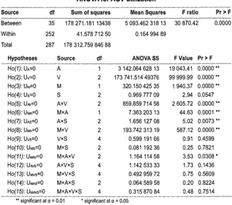
To obtain a 95% confidence interval for the sample mean, eight replications per simulation are run (Pritsker et a/.,1997). One week of seven days, 24 hoyrs per day, is used as the observation period. Run lengths of the same magnitude or les~ have been used in previous flexible manufacturing simulation studies (Stecke and Solberg, 1981; Shanker and Tzen, 1985; Chang eta/., 1986; Choi and Malstrom, 1988; Ozden, 1988). The inter-arrival distribution generates a mean of 21 parts per hour, therefore it is estimc.ted that approximately 3500 parts enter the system over the one week time span. The observation period for each replication is set at 3500 processed parts with data gathered for this number of parts processed following the establishment of the steady state. After reaching the steady state, statistical arrays are cleared while leaving the state of simulated system intact. The main study consists of a full factorial model of all four factors simulated for eight replications. The response variable, AGV utilization (U), is collected for the 3500 completed parts. The total output is made up of 288 observations. No major departures from normality were found, and because all ni=8 (i=1, 2, ... ,36), the model I (fixed factor levels) of the analysis of variance (ANOVA) (Eisenhart, 194 7) will be used to analyse the data. Average machine utilization approaches 70% over all experimental conditions ranging between 69.74% and 69.80%. The factor settings do not significantly affect the overall shop utilization. The analysis of variance results for AGV utilization are displayed in Table IV.

(11)

PoRTUGUESE JOURNAL OF MANAGEMENT STUDIES, VOL. XVI, NO.· 2, 2011 TABLE IV

ANOVA _forAGV _utilization

---Source df Sum of squares

Between

Within

Total

35 178 271.18113438

252 41.578 712 50

287 178 312.759 846 88

Hypotheses Source df

Ho(1 ): UA=O A

Ho(2): Uv=O V 2

Ho(3): UM=O M 1

Ho(4): Us=O S 2

Ho(5): UAv=O AxV 2

Ho(6): UMA=O MxA 1

Ho(7): UAs=O AxS 2

Ho(B): UMv=O MxV 2

Ho(9): Uvs=O VxS 4

Ho(10): UMs=O MxS 2

Ho(11): UMAv=O MxAxV 2

Ho(12): UAvs=O AxVxS 4

Ho(13): UMvs=O MxVxS 4

Ho(14): UMAs=O MxAxS 2

Ho(15): UMAvs=O MxAxVxS 4

Mean Squares

5 093.462 318 13

0.164 994 89

ANOVASS

3 142.064 628 13 173 741.51449376 320.150 425 35 0.969 777 09 859.859 714 58 7.363 203 13 1.656 127 08 193.742 313 19 0.599 191 66 0.08119236 1.164114 58 1.142 533 33 0.492 959 72 0.064 589 58 0.315 870 84

" significant at a= 0.01 • significant at a = 0.05

F ratio Pr> F

30 870.42 0.0000

F Value Pr> F

19043.41 0.0000 **

99 999.99 0.0000 **

1 940.37 0.0000 **

2.94 0.0547

2 605.72 0.0000 **

44.63 0.0001 **

5.02 0.0073 **

587.12 0.0000 **

0.91 0.4599 0.25 0.7821 3.53 0.0308. 1.73 0.1436 0.75 0.5609 0.20 0.8224 0.48 0.7514

Automated guided vehicle utilization is significantly impacted by the assignment rule (A), number of AGVs (V) and machine commonality (M). As expected, AGV utilization decreases as the number of vehicles is increased. The OOM assignment rule generates lower AGV utilization than does WINO as the OOM was designed to decrease time in system by minimizing the part movement among MTs. The high commonality product mix results in lower AGV demand than the low commonality factor setting. Part sequencing rule (S) has little impact on AGV utilization. MxAxV is the highest order interaction that is statistically significant. We then studied MxA at all levels of V; MxV at all levels of A; and AxV at all levels of M. Results show that AGV utilization is higher when three vehicles are used regardless of how machine commonality and the assignment rule are set. Table V displays the AGV utilization for the MxAxV interaction.

3AGV

5AGV

7AVG

TABLEV

AGV _utilization

Low machine commonality

OOM 77.05 78.67 78.36 WINQ 39.21 66.70 62.16

High machine commonality

(12)

PORTUGUESE JOURNAL OF MANAGEMENT STUDIES, VOL. XVI, NO. 2, 2011

The highest AGV utilization levels result from combining the WINO rule with three vehicles at either high or low machine commonality, whereas the lowest levels of utilization result when OOM is selected as the assignment rule combined with a seven vehicle fleet. It is found that the average utilization decreases at a similar rate regardless of how machine commonality and assignment rule are combined. Table VI shows the utilization decrease.

3 versus 5 AGVs

5 versus 7 AGVs

TABLE VI

Decrease(%) of AGV utilization

Low machine commonality High machine commonality

OOM

48.72

34.46

WINO

49.45

34.66

OOM

47.59

33.82

WINO

48.50

33.94

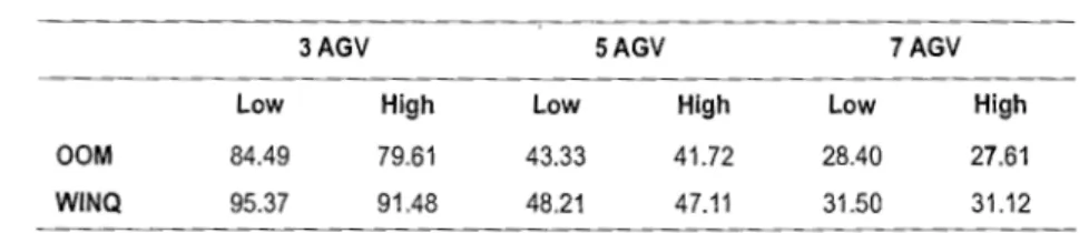
The assignment rule has a strong impact on AGV utilization. For every combination of number of vehicles and machine commonality factors, utilization increases as the assignment rule is changed from OOM to WINO, as shown in Table VII. The increase in utilization ranges from 1 0. 92 % with a fleet of seven vehicles at the low level of machine commonality to nearly 15% with three vehicles at the high level of machine commonality. From Table VII, it is apparent that AGV utilization decreases as the machine commonality shifts from low to high level for any combination of assignment rule and number of AGVs.

TABLE VII AGV utilization

3AGV SAGV 7AGV

Low High Low High Low High

OOM 84.49 79.61 43.33 41.72 28.40 27.61

WINO 95.37 91.48 48.21 47.11 31.50 31.12

The interaction AxS is the only first order that has a factor, S, neither present in the statistically significant higher second order interaction nor significant by itself as a main factor. Table VIII shows that the highest utilization is obtained under the treatment WINOxSPT. Nonetheless, this AGV utilization mean is not statistically different from the other two means observed for the WINO assignment rule. The lowest AGV utilization is observed when OOM assignment rule is combined with the SPT/TOT sequencing rule. This result is not significantly different from the mean observed for the treatment OOMxSPT. Nevertheless, the mean for the treatment OOMxMOPP is found to be statistically different from all other means.

(13)

SPT/TOT

50.76

PORTUGUESE JOURNAL OF MANAGEMENT STUDIES, VOL. XVI, NO. 2, 2011 TABLE VIII

AGV utilization

MOPP

51.03

SPT/TOT

57.41

MOPP

57.43

The analysis of the average machine utilization controlled for assignment rule, number of AGVs, and machine commonality shows that for every treatment combination, the WINO maximum machine utilization were lower than those generated by OOM as shown in Table IX. In every case, the maximum utilization imbalance associated with WINO is smaller than the correspondent OOM imbalance. For instance, the five AGV high machine commonality maximum difference for the OOM assignment rule is 84.75 (=99.82-15.07) while the corresponding WINO difference is 66.58. For a given AGV fleet, variation among machines is more levelled under WINO than under OOM (Table X).

TABLE IX

Average machine utilization

OOM WINQ OOM WINQ

3AGV

Machine 1 55.65 75.62 57.28 79.50

Machine 2 97.52 82.52 95.03 85.26

Machine 3 80.26 73.86 81.48 74.78

Machine 4 94.89 73.70 99.79 75.95

Machine 5 20.47 43.31 15.24 33.36

Overall 69.76 69.80 69.76 69.77

Std. Dev. 32.18 15.24 34.66 20.76

5AGV

Machine 1 55.14 80.70 56.95 84.74

Machine 2 98.62 92.79 95.41 91.53

Machine 3 80.08 76.65 81.27 74.16

Machine 4 95.03 72.40 99.82 73.35

Machine 5 19.95 26.09 15.07 24.95

Overall 69.76 69.73 69.70 69.75

Std. Dev. 32.68 25.55 34.82 26.17

----·-·--·--··- . ---~---~---·· ·-·-______________ .. __

7AGV

Machine 1 55.23 80.64 57.46 85.21

Machine 2 98.66 93.83 95.44 92.50

Machine 3 79.94 73.20 80.73 72.33

Machine 4 94.73 69.36 99.82 67.60

Machine 5 20.30 31.67 15.16 31.07

Overall 69.77 69.74 69.72 69.74

Std. Dev. 32.48 23.24 34.70 23.79

---··--·-···-··-- ______ .. ____

(14)

PORTUGUESE JOURNAL OF MANAGEMENT STUDIES, VOL. XVI, NO. 2, 2011

However, when comparing across the three fleets, for both low machine and high machine commonality levels, the maximum machine utilization imbalance is more levelled under OOM than under WINO, as shown in Table X.

3AGV

5AGV

7 AVG

TABLE X

Maximum machine utilization imbalance

OOM

77.05

78.67

78.36

WINO

39.21

66.70

62.16

OOM

84.55

84.75

84.66

WINO

51.90

66.58

61.43

This maximum imbalance always occurs between the fleets of three and five AGVs. When machine commonality is set at the low level, the maximum imbalance variation is 2.10% under OOM and 70.1% under WINO. At the high level of machine commonality, the maximum imbalance variation is 0.24% under OOM and 28.29% under WINO.

The tendency of OOM to overload machines capable of entirely processing a part is illustrated by the utilization of machine four when machine commonality is set at the high level. At the high level, seven out of ten parts can entirely be processed on one machine and machine four can process five of these seven parts. The results exhibit a nearly full utilization for machine four. At the low level of machine commonality, the highest machine utilization levels under: OOM are associated with machines two and four, which are capable of entirely processing parts E and F, and F and H, respectively. Machine utilization is as high as 98.66% for machine two and 95.03% for machine four. The shorter transport time resulting from the OOM assignment rule is more than counteracted by the increased queue delays generated by machine workload imbalances and extremely high maximum utilizations.

Exploratory analysis is performed to see how the system would respond to a change in the capacity of MT input and output queues and to an increase in the number of AGVs to eight, nine and 10 vehicles. Decreasing the MT input and output queue capacities to only three slots resulted in total system stoppage because the system was incapable of handling peak demand times. AGVs had parts to pick up, but no place to drop them off. Increasing the MT queue slots to five gives the system enough work in progress storage space to avoid the blockages generated during the peak demand periods. Increasing the size of the MT queues beyond five has no further impact on the system.

It is expected that the mean AGV utilization will decrease with each additional vehicle. All treatments used to perform the exploratory analysis show that the AGV utilization consistently decreases as the number of AGVs increases from eight to nine and then to 10. Decreases in AGV utilization range from 10.77% to 13.01%.

(15)

CONCLUSIONS

This research used simulation to evaluate the performance of a dedicated FMS made up of five machines to process ten different parts. Parts' movements among machines were made by mean of a fleet of AGVs. Performance of the system was measured with respect to AGV utilization under thirty-six different configurations.

Automated guided vehicle utilization was found to increase as the number of vehicles decreases. Results showed that WINQ requires more transfers among machines and therefore higher AGV utilization compared to OOM assignment rule. Higher AGV utilization was found to be associated with the low level of machine commonality because at this level the number of parts requiring processing in more than one machine is higher than at the high level of machine commonality, therefore putting a higher demand' on the AGV fleet. Sensitivity analysis demonstrated that system performance was adversely affected not only by too many AGVs but also surplus queue spots. The decay in system performance associated with an increase from five to seven AGVs was observed to continue as the number of vehicles was increased to ten.

In spite of negligible variation across the overall machine utilization, remarkable variation was found among the five machines for both OOM and WINO. Variation among machines was found to be more levelled under WINO than under OOM within the same AGV fleet; nonetheless, maximum machine imbalance is more levelled under OOM when the comparison is made across the fleets.

(16)

REFERENCES

AIDurgham, M.M. and Barghash, M.A. (2008). A generalised framework for simulation-based decision support for manufacturing, Production Planning & Control, 19 (5), pp. 518-534. Bischak, D.P. and Stevens, K.B. (1995). An evaluation of the tandem configuration automated guided vehicle system. Production Planning & Control, 6 (5), pp. 438-444. Chan, F. (2002). Evaluation of combined dispatching and routing strategies for a flexible

manufacturing system. Proceedings of the Institution of Mechanical Engineers, Part B. Journal of Engineering Manufacture, 216 (7}, pp. 1033-1046.

Chan, F.T.S. (2002). Evaluation of combined dispatching and routeing strategies for a flexible manufacturing system. Proceedings of the Institution of Mechanical Engineers, Part B, 216, pp. 1033-1046.

Chang, Y-L., Sullivan, R., and Wilson, J. (1986). Using SLAM to design the material handling system of a fle~ible manufacturing system. International Journal of Production Research, 24 (1), pp. 15-26.

Chen, I.J. and Chung, C-S. (1996). Sequential Modeling of the Planning and Scheduling of Flexible Manufacturing Systems. Journal of the Operational Research Society, 47, pp. 1216-1227.

Choi, R.H. and Malstrom, E.M. (1988). Evaluation of traditional work scheduling rules in a flexible manufacturing system with a physical simulator. Journal of Manufacturing Systems, 7 (1 ), pp. 33-45.

Conway, R.W. (1963). Some tactical problems in digital simulation. Management Science, 10 (1), pp. 47-61.

Denzler, D.R. and Boe, W.J. (1987). Experimental investigation of flexible manufacturing system scheduling decision rules. International Journal of Production Research, 25 (7), pp. 979-994.

Dhouib, K., Gharbi, A., and Ayed, S. (2009). Simulation based Throughput Assessment of Non Homogeneous Transfer Lines. International Journal of Simulation Modelling, 8 (1), pp. 5-15.

Eisenhart, C. (1947). The assumptions underlying the analysis of variance. Biometrics, 3 (1 ), pp. 1-21.

Elsayed, E.A. and Boucher, T.O. (1985). Analysis and Control of Production Systems. Englewood Cliffs: Prentice-Hall.

Gunther, H.O., Gronalt, M., and Zeller, R. (1998). Job sequencing and component set-up on a surface mount placement machine. Production Planning & Control, 9 (2), pp. 201-211. Iwata, K., Murotsu, A., Oba, F., Yasuda, K., and Okamura, K. (1982). Production scheduling of flexible manufacturing systems, CIRP Annals- Manufacturing Technology, 31 (1 ), pp. 319-322.

Kuzgunkaya, 0. and EIMaraghy, H.A. (2007). Economic and strategic perspectives on investing in RMS and FMS, International Journal of Flexible Manufacturing Systems. 19 (3), pp. 217-246.

Lee, K., Shin, J. G., and Ryu, C. (2009). Development of simulated-based production execution system in a shipyard: a case study for a panel block assembly shop. Production Planning & Control, 20 (8), pp. 750-768.

Miller, R.K. and Subrin, R. (1987). Automated guided vehicles and automated manufacturing, Society of Manufacturing Engineers, Dearborn, Michigan

Nance, R. and Sargent, R. (2002). Perspectives on the evolution of simulation. Operations Research, 50 (1), pp. 161-172.

(17)

Ozden, M. (1988). A simulation study of multiple-load-carrying automated guided vehicles in a flexible manufacturing system. International Journal of Production Research, 26 (8), pp. 1353-1366.

Pritsker, A.A., O'Reilly, J.J., and LaVal, D.K. (1997). Simulation with Visual SLAM and AweSim. New York: John Wiley & Sons.

Reddy, B.S.P. and Rao, C.S.P. (2006). A hybrid multi-objective GA for simultaneous scheduling of machines and AGVs in FMS. International Journal of Advanced Manufacturing Technology, 31 (5/6), pp. 602-613.

Sabuncuoglu, 1., and Hommertzheim, D.L. (1989). An investigation of machine and AGV scheduling rules in an FMS, Stecke, K.E.; Suri, R. (Editors), Proceedings of the 3rd ORSA/TIMS Conference on Flexible Manufacturing Systems: operations research models and applications, pp. 261-266

Sarin, S.C. and Chen, C.S. (1987). The machine loading and tool allocation problem in a flexible manufacturing system. International Journal of Production Research, 25 (7), pp. 1081-1094.

Sarma, U.M.B.S., Kant, S., Rai, R., and Tiwari, M.K. (2002). Modelling the machine loading problem of FMSs and its solution using a tabu-search-based heuristic. International Journal of Computer Integrated Manufacturing, 15 (4 ), pp. 285-295.

Shang, J. and Sueyoshi, T. (1995). A unified framework for the selection of a Flexible Manufacturing System. European Journal of Operational Research, 85 (2), pp. 297-315. Shanker, K. and Tzen Y-J. (1985). A loading and dispatching problem in a random flexible manufacturing system. International Journal of Production Research, 23 (3),pp. 579-595. Singh, N., Sarngadharan, P. V., and Pal, P. K. (2011). AGV scheduling for automated material

distribution: a case study. Journal of Intelligent Manufacturing, 22, pp. 219-228. Sridharan, R. and Babu, A.S. (1998). Multi-level scheduling decisions in a class of FMS using

simulation based metamodels. Journal of the Operational Research Society, 49 (6), pp. 591-602.

Stecke, K.E. and Solberg, J.J. {1981). Loading and control policies for a flexible manufacturing system. International Journal of Production Research, 19 (5), pp. 481-490. Um, 1., Cheon, H., and Lee, H. (2009). The simulation design analysis of a flexible

manufacturing system with automated guided vehicle system. Journal of Manufacturing

Systems, 28, pp. 115-122.

Yeh, M.-S., and Yeh, W.-C. (1998). Deadlock prediction and avoidance for zone-control AGVS. International Journal of Production Research, 36 (10), pp. 2879-2889.

Yun, W. Y., Moon, 1., and Kim, G. (2008). Simulation-based maintenance support system for multi-functional complex systems. Production Planning & Control, 19 (4), pp. 365-378.

(18)