Thoft-Cristensen [5] proposed a model using the reliability index as an indicator of the performance of an individual bridge under no maintenance as: () ()( )

Abstract

In developed countries, civil infrastructures are one of the most significant investments of governments, corporations, and individuals. Among these, transportation infrastructures, including highways, bridges, airports, and ports, are of huge importance, both economical and social. Most developed countries have built a fairly complete network of highways to fit their needs. As a result, the required investment in building new highways has diminished during the last decade, and should be further reduced in the following years. On the other hand, significant structural deteriorations have been detected in transportation networks, and a huge investment is necessary to keep these infrastructures safe and serviceable. Due to the significant importance of bridges in the serviceability of highway networks, maintenance of these structures plays a major role.

In this paper, recent progress in probabilistic maintenance and optimization strategies for deteriorating civil infrastructures with emphasis on bridges is summarized. A novel model including interaction between structural safety analysis, through the safety index, and visual inspections and non destructive tests, through the condition index, is presented. Single objective optimization techniques leading to maintenance strategies associated with minimum expected cumulative cost and acceptable levels of condition and safety are presented. Furthermore, multi-objective optimization is used to simultaneously consider several performance indicators such as safety, condition, and cumulative cost. Realistic examples of the application of some of these techniques and strategies are also presented.

1

Introduction

Due to increasing deterioration of existing bridges, a need for systematically addressing the prioritization of maintenance actions on existing civil infrastructures arose during the late 1960s and the 1970s. This was first addressed by Departments of Transportation in the United States, resulting in implementation of a set of computer-based management systems.

Currently available bridge management systems, including PONTIS [1] and BRIDGIT [2], are directly related to the condition states of bridge elements. The number of condition states is limited (e.g., five) for each bridge element. Each condition describes the type and severity of element deterioration in visual terms. Poorer conditions indicate the need for more extensive maintenance actions [3]. PONTIS and BRIDGIT assume that the condition states incorporate all the information necessary to predict future deterioration and use a Markovian deterioration model to predict the annual probability of transition among condition states [1,2]. This is a quite simple approach requiring relatively limited computational power. The approach is also intuitive, as it relates the need for maintenance with aspects that can be visually observed.

As indicated in [4], the Markovian approach used in currently available bridge management systems has several important limitations, such as: (a) severity of deterioration is described in visual terms only; (b) condition deterioration is assumed to be a single step function; (c) transition rates among condition states of a bridge element are not time dependent; and (d) bridge system condition deterioration is not explicitly considered. Experience gained in different countries shows that the major part of the work on existing bridges depends on the load carrying capacity (or structural reliability) of the bridge system rather than the condition states of the bridge elements alone [4]. The use of condition state as the only indicator of the performance of a structure can be misleading. In fact, structural defects that are not visible and/or not discovered by visual inspections can be extremely detrimental to the structural safety. Furthermore, results of visual inspection can be significantly influenced by the experience of the inspectors, accessibility to the structure, and recent repairs that might have hidden existing defects. Consequently, bridge management systems have to also consider the load carrying capacity (or structural reliability) deterioration.

2

Reliability-based approach

2.1

Reliability deterioration under no maintenance

Thoft-Cristensen [5] proposed a model using the reliability index as an indicator of the performance of an individual bridge under no maintenance as:

( )

_{( ) (}

( )

₎

⎩

⎨ ⎧

> −

−

≤ ≤ =

I I

I

t t t

t

t t t

if 0

0 if 0

α β

β

β (1.a)

(1.b) where β

( )

t is the time-dependent reliability index, tI is the time of initiation of

deterioration of reliability index, αis the deterioration rate of reliability index, and t

is time.

As clearly indicated by Shetty and Chubb [6], typical reliability profiles for various failure modes (e.g., bond and shear of reinforced concrete crossbeams) decrease non-linearly with time. For this reason, capturing the non-linear effect of reliability deterioration is clearly of paramount importance. Therefore, the linear model above was extended into the non-linear range by Petcherdchoo and Frangopol [7]. In order to exemplify the effect of non-linear deterioration of the mean reliability index, Figure 1 [7] shows five cases, including both linear (Case 1), and non-linear deterioration (Cases 2 to 5). These cases are all associated with the mean reliability index profile of steel/concrete composite bridges in bending under no maintenance. The mean linear profile in Figure 1 is defined in [8-10].

β= β0−α1(t−tI)

β= β0−α2(t−tI)2

β= β0−α3(t−tI)0.5

β= β₀−α₄(t−t_I)−α₅(t−t_I)2

β= β0−α6(t−tI)−α7(t−tI)0.5

50,000 SAMPLES 2 CASE 1

3

4

5

1 2 4

3 5

2.2

Reliability deterioration under maintenance

In 1998, Frangopol [9] proposed a model using reliability index as a measure of performance of deteriorating structures under the effect of maintenance actions. The proposed model considers linear deterioration under no maintenance as proposed by Thoft-Cristensen [5]. The effects of maintenance actions are modeled through an improvement in reliability immediately after application and a reduction of the deterioration rate for a period of time after application. The eight random variables defining the model are as follows: initial reliability index, B0; time of damage

initiation, TI; reliability deterioration rate without maintenance, A; time of first

application of preventive maintenance, TPI; time of reapplication of preventive

maintenance, TP; duration of preventive maintenance effect on bridge reliability,

TPD; reliability deterioration rate during preventive maintenance effect, Θ ; and

improvement of reliability index (if any) immediately after the application of preventive maintenance, Γ. The two distinct maintenance regimes (i.e., reliability profile with and without preventive maintenance actions) shown in Figure 2 [8,9] are identified through particular values β0, tI, α, tPI, tP, tPD, θ, and γ of the random

variables B0, TI, Α, TPI, TP, TPD, Θ, and Γ, respectively.

BRIDGE AGE, YEARS

γ

γ

γ

1

θ

WITH PREV. MAINT.

1

WITHOUT PREV. MAINT.

R

RP

REHABILITATION TIME , t

REHABILITATION TIME , t

t

β

RELIABILITY INDEX,

I

)

(t

)

(t

f

f

β

o

PI

t

_t

_P

_t

_P

_t

_P

PD

t

PD

t

PD

t

β

target

θ

1

α

₁

1

α

₁

1

α

₁

Figure 2: Reliability profile under the effect of cyclic maintenance actions [8,9]. The time-dependent reliability index under maintenance can be analytically computed as described in [7]. If the profile without maintenance is defined as shown in Case 4 of Figure 1, then:

( )

_{( )}

_{( )}

⎩ ⎨ ⎧

− −

= 2

0 t-t α t-t α β

β t

β I

t t

t t

> ≤ ≤

if 0 if

, (2.a)

Six different cases, depending on the time of application of maintenance must be considered as follows:

Case 4a ⎩ ⎨ ⎧ > ≤ PD P PI I t t t t (3.a) (3.b)

Case 4b _⎩⎨

⎧ ≤ ≤ PD P PI I t t t t (4.a) (4.a) Case 4c

( )

( )

⎩ ⎨ ⎧ > + + ≤ < + PD P PD P PI * I P PI t t t t m-t t t

m-t 1 1 (5.a)

(5.b) Case 4d

( )

( )

⎩ ⎨ ⎧ ≤ + + ≤ < + PD P PD P PI I P PI t t t t m-t t t

m-t 1 * 1 _(6.a)

(6.b) Case 4e

( )

⎩ ⎨ ⎧ > + ≤ < + + PD P P PI * I PD P PI t t mt t t t t

m-t 1 (7.a)

(7.b)

Case 4f

( )

⎩ ⎨ ⎧ ≤ + ≤ < + + PD P P PI * I PD P PI t t t m t t t t

m-t 1 (8.a)

(8.b)

where I PDη

*

I t mt

t = + is the time of damage initiation considering maintenance,

m = number of maintenance actions applied before damage initiation, and η = factor representing the effectiveness of maintenance on the extension of time of damage initiation (0 ≤η≤ 1). In the present study, η = 0.5. As an example, for Case 4a (see eqns. (3.a) and (3.b)), the reliability profile under maintenance shown in Figure 3 [7] is as follows:

0

β (9.a)

(

)

(

)

2

5 4

0 α t tI α t tI

β − − − − (9.b)

(

t tPI

)

θ

β1− − (9.c)

(

)

[

] [

]

{

}

(

)

[

] [

]

{

}

2

1 1 5 1 1 4 * 1 I I PD PI I I PD PI t t t t t t t α t t t t t t t α β − − − − + − − − − − − + − − (9.d)

(

)

[

]

{

PI P

}

n θ t t n t

β − − + −1 (9.e)

( )

⎪ ⎪ ⎪ ⎪ ⎪ ⎪ ⎪ ⎪ ⎩ ⎪ ⎪ ⎪ ⎪ ⎪ ⎪ ⎪ ⎪ ⎨ ⎧ = t β

(

)

(

)

[

] [

]

{

}

(

)

(

)

[

] [

]

{

}

2

5 4 * 1 1 I n I n PD P PI I n I n PD P PI n t t t t t t n t t α t t t t t t n t t α β − − − − + − + − − − − − − + − + − − (9.f) where n = number maintenance applications before time t, and

(

t t

)

α

(

t t

)

γ α

β

β = − PI − I − PI − I +

2 5

4 0

PD

t θ β

β = 1−

*

1 (11)

[ ] [

]

{

t -t t t

}

α

{

[ ] [

t -t t t

]

}

γ

α β

βn= n− − I − − I − I − − I +

2 1 * 1 5 1 * 1 4 *

1 att=tPI +

(

n−1

)

tP (12)

PD n *

n β θt

β = − att=t_PI +

(

n−1

)

t_P+t_{PD (13)}

where

(

)

[

]

5 5 0 * 1 0 5 2 4 4 1 2α β β α α α t t . n I − − − + − + = (14)

(

)

[

]

5 5 0 * 0 5 2 4 4 2α β β α α α t t . n I n − − + − + = (15)

(

)

[

]

[

(

)

]

{

1

}

*

1 t n 1t t n 2t t t

t = _PI + − _P − _PI + − _P+ _PD− (16)

PD

t

PD

t

t

P P

t

P

t

o β

t

PD PI ) tP (γ γ ) Γ f Α 4 (α 4 ) f 4 α t RELIABILITY INDEX,

BRIDGE AGE, YEARS

γ

WITH PREV. MAINT.

WITHOUT PREV. MAINT.

β R RP

t

I γ θ 1 1 θ γ

REHABILITATION TIME, t

REHABILITATION TIME, t

P (t tRP ) fT RP RP fΤ Ι (tI ) tI βtarget

(t−tI)

α4

βo− −α5(t−tI)2

tR

R

)

(t

fTR

α Τ PI ) fΤ PD ) PD (t tPD fΘ (θ) θ fΤ P (t f 5 5 ) f 5 Α (α Β ο f (β o ) βo tPI (tPI

Figure 3: Reliability index profile without and with preventive maintenance associated with Case 4a [7]

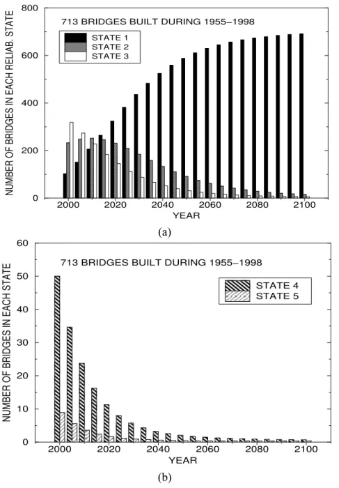
Figure 4 shows the prediction of the evolution in time of the number of bridges in each reliability state from a stock of 713 bridges built during 1955-1998 under no maintenance. Reliability states are defined as: excellent (i.e., state 5, where β ≥ 9.0); very good (i.e., state 4, where 9.0 > β ≥8.0); good (i.e., state 3, where 8.0 > β ≥ 6.0); fair (i.e., state 2, where 6.0 > β ≥ 4.6); and unacceptable (i.e., state 1, where β < 4.6). Figure 5 shows the effect of preventive maintenance on the evolution in time of the number of bridges in each reliability state.

2000 2020 2040 2060 2080 2100

YEAR 0

200 400 600 800

NUMBER OF BRIDGES IN EACH RELIAB. STATE

STATE 1 STATE 2 STATE 3

713 BRIDGES BUILT DURING 1955−1998

(a)

2000 2020 2040 2060 2080 2100

YEAR 0

10 20 30 40 50 60

NUMBER OF BRIDGES IN EACH STATE

STATE 4 STATE 5 713 BRIDGES BUILT DURING 1955−1998

(b)

2000 2020 2040 2060 2080 2100 YEAR

0 200 400 600 800

NUMBER OF BRIDGES IN EACH RELIAB. STATE

STATE 1 STATE 2 STATE 3

713 BRIDGES BUILT DURING 1955−1998 WITH PREV. MAINT.

(a)

2000 2020 2040 2060 2080 2100

YEAR 0

10 20 30 40 50 60 70 80

NUMBER OF BRIDGES IN EACH STATE

STATE 4 STATE 5 713 BRIDGES BUILT DURING 1955−1998

WITH PREV. MAINT.

(b)

The main advantage of the reliability-based methodology is the use of a consistent measure of safety, as the reliability index, instead of the condition state. Furthermore, the use of continuous performance profiles allows the incorporation of the reduction of deterioration rate caused by maintenance actions. This methodology however, does not incorporate information resulting from visual inspections on bridges. Furthermore, some reluctance was found in applying this methodology as bridge managers prefer not to abandon the condition states as a part of the bridge management system.

2.3

Survivor Function Model

Survivor functions have been proposed as a tool for bridge management systems by Yang et al. [11,12] and van Noortwijk et al. [13]. The probability of survival, Ps , of

a deteriorating component under no maintenance decreases with time t according to a function dependent on the type of component, quality of construction, and environmental conditions, among others. Ps can be approximated by various lifetime

distribution functions (LDFs) [14]. These functions must satisfy the following conditions:

Ps = 1 at t = 0 (17)

Ps = 0 at t →∞ (18)

0

s

P t

∂ _≤

∂ (19)

The survivor functions are a simpler way of modeling the non-linear time-dependent probability of failure, including the effect of preventive and essential maintenance actions. Yang et al. [11,12] consider exponential and Weibull functions lifetime distribution functions, defined as, respectively:

( )

t s

P =S t =e−λ (20)

( )

( )_st s

P S t e

κ λ −

= = (21)

If a structural system can be reduced to a series-parallel system of independent components its survivor function can be computed in a simple manner. In fact, the probability of survival of a sub-system of n independent components associated in parallel or series is given, respectively, as:

( )

_∏

(

( )

)

=

− −

= n

i

i t

S t

S

1 1

1 (22)

( )

_∏

( )

=

= n

i i t

S t

S

1

(23) where S_i

( )

t = probability of survival of component i.

component to its initial value (i.e., at t = 0) [14]. As an example, a series-parallel system composed of three components where components 1 and 2 are associated in series and subsystem 1-2 is associated in parallel with component 3, is analyzed. All components have the same survivor function, characterized by an exponential distribution with λ = 0.0005/year. The probability of failure under no maintenance can be derived, using equations (22) and (23), as:

( )

( ) ( )

( )

0.0005 0.0005 0.0005

1 2 3

1 1 1 1 1 t t 1 t

S t = − −_⎣⎡ S t S t _{⎦ ⎣}⎤ ⎡ −S t ⎤_⎦= − −_⎣⎡ e− e− ⎤ ⎡_{⎦ ⎣} −e− ⎤_⎦ (24) At year 15, component 3 is replaced and its age after year 15 is t-15. At year 30, component 1 is replaced and at year 50 all components are replaced. The resulting system survivor function is:

(25.a) (25.b) (25.c) (25.d)

( )

(

) (

)

(

)

(

( )

)

( )

(

)

(

( )

)

( ) ( )

(

)

(

( )

)

⎪ ⎪ ⎩ ⎪ ⎪ ⎨ ⎧ ≥ − − − < ≤ − − − < ≤ − − − < − − − = − − − − − − − − − − − − − − − − − − years 0 5 1 1 1 years 50 years 0 3 1 1 1 years 30 years 15 1 1 1 years 15 1 1 1 50 0005 . 0 50 0005 . 0 50 0005 . 0 15 0005 . 0 0005 . 0 30 0005 . 0 15 0005 . 0 0005 . 0 0005 . 0 0005 . 0 0005 . 0 0005 . 0 t e e e t e e e t e e e t e e e t S t t t t t t t t t t t t

The survivor function method allows for a simple computation of the probability of failure of deteriorating structures under essential, proactive, and/or reactive maintenance actions [11]. This methodology was also used to optimize the maintenance actions on an existing bridge [11] based on data compiled by Maunsell Ltd. [15]. However, the capabilities of the methodology are limited in modeling the effects of different maintenance actions.

3

Condition-Safety Approach

Frangopol and Neves [16] proposed an extended model that integrates the currently used condition states with structural safety. In addition to the previously described reliability-based model (see Figure 2), a new parameter defining a period during which no deterioration occurs after the application of maintenance is also included. The interaction between condition and safety is taken into account in two different manners: (a) correlation between parameters; and (b) deterministic relations between the value of one performance indicator and the deterioration of the other. Correlation between parameters occurs, for example, between the deterioration rates of condition and safety. In fact, under an aggressive environment both condition and safety will deteriorate faster than in a less aggressive environment.

3.1

Condition and safety profiles

The condition index and safety index profiles under no maintenance are each defined using three random variables: initial condition and safety, C0 and S0,

respectively; time of initiation of deterioration of condition and safety, ti and tic,

Each maintenance action can lead to one, several, or all of the following effects: (a) increase in the condition index and/or safety index immediately after application; (b) suppression of the deterioration in condition index and/or safety index during a time interval after application; and (c) reduction of the deterioration rate of condition index and/or safety index during a time interval after application. These effects are modeled through several random variables as follows: (a) increase in condition index and safety index immediately after application, γc and γ, respectively; (b) time

during which the deterioration processes of condition index and safety index are suppressed, tdc and td, respectively; (c) time during which the deterioration rate in

condition index and safety index are suppressed or reduced, tpdc and tpd, respectively;

and (d) deterioration rate reduction of condition index and safety index , δc and δ,

respectively. The meaning of each of these variables is indicated in Figures 6 and 7 , for condition and safety, respectively.

tic

γc

tdc

α δc- c

αc

profile under no maintenance

profile under maintenance

TIME

CO

NDIT

ION INDEX,

C

tpdc

tpi tp

C₀

tp

Figure 6: Condition index profile without or with maintenance [17].

1

γ td

α δ

-α

profile under no maintenance

profile under maintenance

TIME

SA

F

ETY

IN

DEX

,

S

tpi tp tp

tpd

ti

S₀

Figure 7: Safety index profile without or with maintenance [17].

Maintenance actions can be classified, according to their time of application as: (a) time-based; (b) performance-based; and (c) time- and performance-based [17]. Time-based maintenance actions are those for which the time of application is defined by deterministic or random variables independent of the performance of the structure. Performance-based maintenance actions are those applied when a condition threshold or/and a safety threshold is reached or violated. Time- and performance-based actions are those for which one or more applications are time-based and the others are performance-time-based. To be able to model a wide range of maintenance actions, the condition and safety profiles are computed considering that the effect of maintenance actions can be superposed on the profile under no maintenance [17-19]. This approach allows the development of a more versatile model, that can be enhanced to include new maintenance profiles.

If not controlled, the use of superposition, together with simulation, might yield erroneous results, such as negative deterioration rates or increase in deterioration rate due to maintenance. These situations were avoided using the algorithm described in the next section. The uncertainties in the condition, safety, and cost profiles are captured by using sampling based on Latin-hypercube method.

1

3.2

Computational platform

The use of sampling required the proposed model to be implemented in a computational platform. The profiles must be computed at discrete time intervals, chosen as one year. To avoid erroneous results as those mentioned in the previous section, the superposition is performed in two steps. In the first step the deterioration rate for each one year interval is computed considering all maintenance actions active during this period. If negative deterioration rates occur, or if one maintenance action results in an increase of deterioration rate, the deterioration rates are corrected. The safety and condition indices at the end of the one year interval are then computed.

The deterioration rate of the safety index, considering maintenance, is computed during each year period as [17]:

(

)

zero reduced no

0

T t t t

ε = ⋅ + α δ− ⋅ + ⋅α (26)

where εT is the equivalent rate of safety index deterioration during year

[

T −1;T

]

,

tzero is the fraction of the year during which there is no deterioration of safety due to

the effect of the maintenance action, treduced is the fraction of the year during which

the deterioration rate of safety is reduced due to the maintenance action, and tno is

the fraction of the year during which there is no effect of the maintenance on safety. The duration of each of these periods is given as [17]:

(

)

(

)

zero min d; max 0; 1 0

t = t τ − τ − ≥

(27)

(

)

(

)

effect min pd; max 0; 1 0

t = t τ − τ − ≥

(28)

(

)

reduced min 1; effect zero

t = t −t

(29) no zero reduced 1

t +t +t = ₍₃₀₎

where τ is the time since maintenance was applied, and teffect is the fraction of the

year during which the maintenance action reduces or eliminate deterioration of safety. Similar expressions for computing the rate of deterioration of condition index can easily be derived as indicated in [17].

In order to compute the condition and safety profiles the time integration of the rate of deterioration, can now be easily performed as follows:

⎩ ⎨ ⎧ < ≤ − + ≥ + = − − year C C C C C T T C T T T 1 0 if year 1 if 1 1 τ γ ε τ ε (31) ⎪⎩ ⎪ ⎨ ⎧ < ≤ + − ≥ − = − − year S S S T T T T T 1 0 if year 1 if 1 1 τ γ ε τ ε (32) where CT and ST are the condition index and safety index at time T, respectively. It

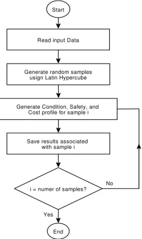
This model was implemented in a Windows platform under a software package named Condition and Reliability Analysis under Maintenance (CRAM). In Figure 8 a very general flowchart describing the implementation of CRAM is shown.

Read input Data

Generate random samples usign Latin Hypercube

Generate Condition, Safety, and Cost profile for sample i

Save results associated with sample i

i = numer of samples?

No

End Start

Yes

Figure 8: General flowchart of simulation process of condition, safety, and cost probabilistic indicators.

3.3

Examples of application

The condition-safety interaction model described was used to assess and predict the future performance of a group of reinforced concrete bridge components in the United Kingdom. Data on the deterioration of these components, in terms of condition and safety, was provided by Denton [20]. For these elements, condition was defined as [20]: 0 – no chloride contamination; 1 – onset of corrosion; 2 – onset of cracking; and 3 – loose concrete/significant delamination. The worst admissible condition index is 3.0. Safety is described according to BD 12/01 [21] as the ratio S

of available to required live load capacity. The minimum acceptable value of S is 0.91.

processes and, consequently, the associated times of initiation of damage of condition and safety, tic and ti, respectively, are zero. The data describing the

condition and safety profiles under no maintenance is shown in Table 1. All random variables are described by triangular distributions.

Condition Index Profile Safety Index Profile

Initial Index Time of Damage

Initiation

Deterioration

Rate Initial Index

Time of Damage Initiation

Deterioration Rate

C0 Tic αc S0 Ti α

(years) (year-1_{) (years) (year}-1₎

(1) (2) (3) (4) (5) (6)

Min = 0.00 Mode = 1.75

Max = 3.50

0.0

Min = 0.00 Mode = 0.08

Max = 0.16

Min = 0.91 Mode = 1.50 Max = 2.5

0.0

Min = 0.00 Mode = 0.015

Max = 0.035

Table 1: Data defining condition and safety profiles under no maintenance [20]. Five maintenance actions were considered for these components: (a) minor concrete repairs; (b) silane; (c) do nothing and rebuild; (d) cathodic protection; and (e) replacement of expansion joints [20]. Of these, minor concrete repair and rebuild are essential maintenance actions, and, consequently, are performance-based. Silane and replacement of expansion joints are preventive maintenance actions, and, consequently, are time-based. Cathodic-protection is time- and performance-based. The effects of each of these maintenance actions on the condition and safety of the components is shown in Tables 2 and 3, respectively.

Effect on Condition Index Maintenance

Strategy

Improve-ment

Delay in Deterioration

Deterioration Rate During Effect

Duration of Maintenance

Effect

γC Tdc αC−δC Tpdc

Cost

(years) (year-1_{) (years) (k£)}

Minor Concrete Repair

2.0 2.5 3.0

0.0 αC 0

16 3605 14437

Silane 0.0 0.0

0.00 0.01 0.03

7.5 10.0 12.5

0.30 39.0 77.0

Do Nothing and Rebuild

to 0.0

10 15 30

αC Tdc

247 7410 28898

Cathodic Protection 0.0 12.5 αC Tdc

19 2604 5189

Replace Expansion

Joints 0.0 0.0

0.00 0.04 0.08

10.0 15.0 30.0

0.7 15 39

All random variables have a triangular distribution, characterized by their minimum, mode and maximum values.

Effect on Safety Index

Maintenance Strategy

Improve-ment

Delay in Deterioration

Deterioration Rate During Effect

Duration of Maintenance

Effect

γ Td α−δ Tpd

Cost

(years) (year-1) (years) (k£)

Minor Concrete

Repair 0.0

while

C < 1 α Td

16 3605 14437

Silane 0.0 0.0

0.00 0.007 0.018

7.5 10.0 12.5

0.30 39.0 77.0

Do Nothing and Rebuild

1.00 1.25 1.50

while

C < 1 α Td

247 7410 28898

Cathodic Protection 0.0 12.5 α Td

19 2604 5189

Replace Expansion

Joints 0.0 0.0

0.00 0.007 0.018

10.0 15.0 30.0

0.7 15 39

All random variables have a triangular distribution, characterized through by their minimum, mode and maximum values

Table 3: Data defining safety profiles under cyclic maintenance [20].

The times of application of these five maintenance actions are presented in Table 4.

Maintenance Strategy

Time of Maintenance Application _Minor

Concrete Repair

Silane

Do Nothing and Rebuild

Cathodic Protection

Replace Expansion

Joints

0 0 7.5 20 Time of Application of First

Maintenance

Tpi

(years)

when

C = 3.0

15

when

S= 0.91

when

C = 2.0

40

10 7.5 20

12.5 10 30

Time of Subsequent Applications

Tp

(years)

when

C = 3.0

15

when

S= 0.91

12.5 40 All random variables have a triangular distribution, characterized through by their minimum, mode and maximum values

Table 4: Times of application of maintenance actions [20].

effect of minor concrete repair, the condition index does not violate its target, but the safety index downcrosses the prescribed threshold within the prescribed time horizon.

0 10 20 30 40 50

4 3 2 1 0

C

TARGET

NO MAINTENANCE

MODE

MODE

C

O

ND

IT

ION

IN

DE

X

,

C

TIME, Years

0 10 20 30 40 50

0.0 0.5 0.91 1.5 2.5

Application Time Application Time

Application Time

S

TARGET MODE

NO MAINTENANCE

MODE

S

A

FE

T

Y

IN

DE

X

, S

TIME, Years

0 10 20 30 40 50

0 2 4 6 8 10

MODE

MODE

CUM

ULAT

IVE COS

T

(x

1000)

TIME, Years

Figure 9: Condition, safety, and cumulative cost profiles under minor concrete repairs, considering all random variables defined by their mode.

(a)

0 10 20 30 40 50

4 3 2 1 0

PDF at year 0

PDF at year 10

PDF at

year 20 PDF at_{year 30} PDF at year 40

WITH MAINTENANCE

MEAN

NO MAINTENANCE ST.DEV.

CO

NDI

T

IO

N INDEX

,

C

TIME, Years

(b)

0 10 20 30 40 50

0.0 0.5 0.91 1.5 3.0

WITH MAINTENANCE

PDF at year 30

PDF at year 20 PDF at

year 10 PDF at

year 0 PDF at

year 40

WITH MAINTENANCE

NO MAINTENANCE

ST.DEV. MEAN

S

A

F

E

T

Y

I

NDE

X

, S

TIME, Years

(b)

0 10 20 30 40 50

0 5 10

ν = 6% ν = 0%

EX

PEC.

CUM

UL.

CO

ST

(

x

1

000

)

TIME, Years

The results show, under no maintenance, a significant deterioration of the mean condition and safety during the entire life, as a result of the aging process. The standard deviations of the condition and safety profiles increase over time, as a result of the high coefficient of variation of the deterioration rates of both condition and safety. These are associated with a significant probability of violating the condition threshold (C = 3.0) at t = 0. For both condition and safety indices, the probability of violating the corresponding target values increases with time.

The comparison of the mean of the condition, safety, and cost profiles in Figures 9 and 10 shows that the inclusion of uncertainties result in smoother mean profiles, without large and/or sudden variations of condition index. Furthermore, the probability density functions (PDFs) represented in Figure 10 show a significant dispersion of the values of the condition and safety indices which is nonexistent in Figure 9. The PDFs shown indicate a zero probability of the condition index violating its threshold, since when this target is reached, maintenance is applied, as condition is improved to zero. However, the probability of the safety index downcrossing its target is significant during the entire lifetime, as a result of the smaller impact of this type of maintenance action on safety.

4

Maintenance optimization

In general, the main objective of a structure manager is to produce a maintenance strategy resulting in minimum maintenance cost, keeping the structure safe and serviceable. Optimization algorithms can be used, together with the model proposed, to reach this goal. In this paper, two major optimization techniques are used: single objective optimization and multi-objective optimization. Single objective optimization has the advantage of a much reduced computational cost as compared with multi-objective optimization. However, multi-objective maintenance optimization allows the analysis of trade-offs between different and conflicting objectives, including condition, safety, and cumulative cost. This will provide the structure manager a set of optimal solutions, from which it is possible to select the best one according to a specific situation, depending on available funds, importance of the structure or group of structures, or impact of failure.

4.1

Single objective maintenance optimization

Figure 11: Flowchart of the optimization process

The design variables considered are the mean time of first application and the mean interval between subsequent preventive maintenance applications. The only constraints considered are the lower and upper bounds of design variables. In general, the lower bound is chosen to prevent realizations associated with negative times of application. The upper bound is selected to allow the resulting time of application to be outside the considered time horizon.

To prevent all samples from violating the condition index and safety index thresholds, combinations of maintenance actions, including one or more preventive actions, rebuild, and minor concrete repair, are employed [23]. In Table 5 the maintenance actions used in each strategy considered for optimization are shown [7].

Strategy Preventive maintenance Essential maintenance 1 Silane Treatment (SL)

2 Cathodic Protection (CP) 3 Replace Expansion Joints

(RJ)

4 SL+RJ 5 CP+RJ

Minor concrete repair (CR)

and Rebuild (RB)

Table 5: Maintenance strategies for condition and safety indices [7].

In Figures 12 and 13 [7] the optimal mean condition and safety profiles for all strategies defined in Table 5 are shown. As indicated, due to the application of essential maintenance actions that prevent both condition and safety from violating

Read general and optimization input files

Do maintenance analysis

Call DOT program for optimization

Use the new values of design variables obtained from DOT as the mean of maintenance application times

Use the present value of expected cumulative maintenance cost as objective function Use mean values of maintenance application

from the target values of 3.0 and 0.91 for condition and safety indices, respectively. The costs associates with the optimal solutions are presented in [7].

0 10 20 30 40 50

TIME (YEARS) 0

1

2

3

4

MEAN OF CONDITION INDEX

NO MAINTENANCE SL + CR +RB CP + CR +RB RJ + CR +RB SL + RJ + CR +RB CP + RJ + CR +RB CONDITION INDEX

WITH OPTIMIZATION MEAN

NO MAINTENANCE

CR : MINOR CONCRETE REPAIR SL : SILANE

RB : REBUILD

CP : CATHODIC PROTECTION RJ : REPLACE EXPANSION JOINTS SL + CR + RB

CP + CR + RB RJ + CR + RB

SL + RJ + CR + RB CP + RJ + CR + RB

TIME HORIZON = 50 YRS. ν = 6%

Figure 12: Optimal mean profile of condition index for the five strategies defined in Table 5 [7].

0 10 20 30 40 50

TIME (YEARS) 0

0.5 1 1.5 2

MEAN OF SAFETY INDEX NO MAINTENANCE_{SL + CR +RB}

CP + CR +RB RJ + CR +RB SL + RJ + CR +RB CP + RJ + CR +RB SAFETY INDEX WITH OPTIMIZATION MEAN

NO MAINTENANCE

SL : SILANE

CP : CATHODIC PROTECTION RJ : REPLACE EXPANSION JOINTS CR : MINOR CONCRETE REPAIR RB : REBUILD

SL + CR + RB CP + CR + RB

RJ + CR + RB SL + RJ + CR + RB

CP + RJ + CR + RB

TIME HORIZON = 50 YRS. ν = 6%

4.2

Multi-objective Optimization

Multi-objective can be used to obtain a set of optimal strategies, in a Pareto optimal sense. This allows the decision maker to find the balance between the three performance indicators that best meets the prescribed needs. Multi-objective optimization was implemented using a genetic algorithm (GA) procedure to solve this problem [24]. This procedure, that emulates Darwin evolution, is particularly adequate to optimize multiple competing objective functions. This approach has, as main advantages, its simplicity and ability to produce, accurately, a large set of optimal solutions. However, it is computational costly, especially if coupled with Monte-Carlo simulation. The process used for joining GA with the condition-safety model is presented in detail in [24]. The problem under analysis can be stated as:

Goal: To obtain a set of optimized trade-off maintenance solutions while 1. minimizing the largest (i.e. worst) condition index during the service life, 2. maximizing the smallest (i.e. worst) safety index during the service life, and 3. minimizing the present value of cumulative life-cycle maintenance cost.

Subject to:

1. condition index ≤ 3.0, 2. safety index ≥ 0.91, and

3. present value of life-cycle cost ≤ life-cycle cost threshold.

The present value of the life-cycle maintenance cost, costPV , is the sum of the

discount costs of all maintenance interventions during the time horizon considered:

(

)

∑∑

= = +

= M

i N

j

t i PV

i

ij

cost cost

1 1 1 ν

(33) where M = number of available different maintenance actions, costi = unit cost

associated with the ith maintenance action; ν = discount rate of money, assumed equal to 6%, Ni = total number of applications of the ith maintenance action during

the life-cycle, tij = time of the jth application of the ith maintenance action. The

design variables considered are the mean times of application of time-based maintenance actions.

5

Conclusions

In this paper, recent progress in probabilistic maintenance and optimization strategies for deteriorating civil infrastructures with emphasis on bridges is summarized. A novel model including interaction between structural safety analysis, through the safety index, and visual inspections and non destructive tests, through the condition index, is presented. This allows a coupling of the state-of-practice with the most recent developments in bridge management and safety analysis. The results obtained show the differences between the two indicators, highlighting the need for the use of both in order to obtain a more accurate prediction of future deterioration of existing civil infrastructures. Single objective optimization techniques leading to maintenance strategies associated with minimum expected cumulative cost and acceptable levels of condition and safety are presented. Furthermore, multi-objective optimization is used to simultaneously consider several performance indicators such as safety, condition, and cumulative cost. Realistic examples of the application of some of these techniques and strategies are also presented. Results presented by the authors and co-workers at the University of Colorado [16-19,23,24] show the crucial role of preventive maintenance actions in reducing the overall maintenance costs, and the need for essential maintenance actions in keeping structures safe and serviceable, during their entire service life.

6

Acknowledgments

The authors gratefully acknowledge the partial financial support of the U.K. Highways Agency and of the U.S. National Science Foundation through grants CMS-9912525 and CMS-0217290. The second author also acknowledges the support of the Portuguese Science Foundation (FCT). The opinions and conclusions presented in this paper are those of the writers and do not necessarily reflect the views of the sponsoring organizations.

References

[1] P.D. Thompson, E.P. Small, M. Johnson, A.R. Marshall “The Pontis bridge management system”, Structural Engineering International, IABSE, 8(4), 303-308, 1998.

[2] H. Hawk, E.P. Small (1998). “The BRIDGIT bridge management system”, Structural Engineering International, IABSE, 8(4), 309-314.

[3] G. Hearn “Condition data and bridge management”, Structural Engineering International, IABSE, (8)3, 221-225, 1998.

[4] P.C. Das “New developments in bridge management methodology”, Structural Engineering International, IABSE, (8)4, 299-302, 1998.

[5] P. Thoft-Christensen “Assessment of the reliability profiles for concrete bridges”, Engineering Structures, 20(11), 1004-1009, 1998.

Future Trends in Bridge Design, Construction and Maintenance”, Thomas Telford, London, 649-660, 1999.

[7] A. Petcherdchoo, D.M. Frangopol “Maintaining Condition and Safety of Deteriorating Bridges by Probabilistic Models and Optimization”, Report No. 04-1, Structural Engineering and Structural Mechanics Research Series No. CU/SR-04/1, Department of Civil, Environmental, and Architectural Engineering, University of Colorado, Boulder, April, 2004, 335 pages, 2004. [8] D.M. Frangopol, J.S. Kong, E.S. Gharaibeh “Reliability-based life-cycle

management of highway bridges”, Journal of Computing in Civil Engineering, ASCE, 15(1), 27-47, 2001.

[9] D.M. Frangopol “A probabilistic model based on eight random variables for preventive maintenance of bridges”, Presented at the Progress Meeting “Optimum Maintenance Strategies for Different Bridge Types”, Highways Agency, London, November, 1998.

[10] J.S. Kong “Lifetime Maintenance Strategies for Deteriorating Structures”, Ph.D. Thesis, Department of Civil, Environmental, and Architectural Engineering, University of Colorado, Boulder, Colorado, 2001.

[11] S-I. Yang, D.M. Frangopol, L.C. Neves “Service life prediction of structural systems using lifetime functions with emphasis on bridges”, Reliability Engineering & System Safety, Elsevier (in press), 2004.

[12] S-I. Yang, E.S. Gharaibeh, D.M. Frangopol and L.C. Neves “System reliability for bridge evaluation and service life prediction” in J.R. Casas, D.M. Frangopol, and A.S. Nowak, eds. “Bridge Maintenance, Safety and Management”, CIMNE, Barcelona, Spain, 9 pages on CD-ROM, 2002.

[13] J.M. van Noortwijk, H.E. Klatter “The use of lifetime distributions in bridge replacememt modeling,” in J.R. Casas, D.M. Frangopol, and A.S. Nowak, eds. “Bridge Maintenance, Safety and Management”, CIMNE, Barcelona, Spain, 8 pages on CD-ROM, 2002.

[14] D. Kececioglu “Maintainability, Availability, & Operational Readiness Engineering”, Vol 1, Prentice-Hall, New Jersey, 1995.

[15] Maunsell Ltd. “Serviceable Life of Highway Structures and their Components - Final Report”, Highways Agency, Birmingham, UK, 1999.

[16] D.M. Frangopol, L.C. Neves “Life-cycle maintenance strategies for deteriorating structures based on multiple probabilistic performance indicators”, System-based Vision for Strategic and Reactive Design, Bontempi F, ed., Sweets & Zeitlinger, Lisse, 1, 3-9 (keynote paper), 2003.

[17] L.C. Neves, D.M. Frangopol “Condition, safety and cost profiles for deteriorating structures with emphasis on bridges”, submitted for publication, 2004.

[18] J.S. Kong, D.M. Frangopol “Life-cycle reliability-based maintenance cost optimization of deteriorating structures with emphasis on bridges”, Journal of Structural Engineering, ASCE, 129(6), 818-828, 2003.

[20] S. Denton “Data Estimates for Different Maintenance Options for Reinforced Concrete Cross Heads”, (Personal communication), Parsons Brinckerhoff Ltd., Bristol, U.K., 2002.

[21] DB12/01 “The Assessment of Highway Bridge Structures”, Highways Agency Standard for Bridge Assessment, London, UK., 2001.

[22] G.N. Vanderplaats “Numerical optimization techniques for engineering design”, Vanderplaats Research & Development, Inc., Colorado Springs, 2001. [23] A. Petcherdchoo, L.C. Neves and D.M. Frangopol “Combinations of

probabilistic maintenance actions for minimum life-cycle cost of deteriorating bridges”, in “Proceedings of the Second International Conference on Bridge Maintenance, Safety, and Management, IABMAS’04”, Kyoto, Japan, October 19-22, (in press) 2004.