Tanya Araújo, Ennes Ferreira

Tanya Araújo, Ennes Ferreira

The Topology of African Exports: emerging

patterns on spanning trees

WP06/2016/DE/UECE/SOCIUS _________________________________________________________

De pa rtme nt o f Ec o no mic s

W

P

The Topology of African Exports: emerging

patterns on spanning trees

Tanya Araújo and M. Ennes Ferreira

ISEG, University of Lisbon Miguel Lupi 20, 1248-079 Lisbon UECE - Research Unit on Complexity and Economics SOCIOUS/CSG - C.I. Sociologia Económica e das Organizações

Abstract

This paper is a contribution to interweaving two lines of research that have progressed in separate ways: network analyses of interna-tional trade and the literature on African trade and development. Gathering empirical data on African countries has important limi-tations and so does the space occupied by African countries in the analyses of trade networks. Here, these limitations are dealt with by the de…nition of two independent bipartite networks: a destination share network and a commodity share network.

These networks - together with their corresponding minimal span-ning trees - allow to uncover some ordering emerging from African exports in the broader context of international trade. The emerg-ing patterns help to understand important characteristics of African exports and its binding relations to other economic, geographic and organizational concerns as the recent literature on African trade, de-velopment and growth has shown.

*Financial support from national funds by FCT (Fundação para a Ciência e a Tecnologia). This article is part of the Strategic Project: UID/ECO/00436/2013

1

Introduction

A growing literature has presented empirical …ndings of the persistent impact of trade activities on economic growth and poverty reduction ([1],[2],[3],[4],[5], [6]). Besides discussing on the relation between trade and development, they also report on the growth by destination hypothesis, according to which, the destination of exports can play an important role in determining the trade pattern of a country and its development path.

Simultaneously, there has been a growing interest in applying concepts and tools of network theory to the analysis of international trade ([7],[8],[9],[10], [11],[12],[13]). Trade networks are among the most cited examples of the use of network approaches. The international trade activity is an appealing ex-ample of a large-scale system whose underlying structure can be represented by a set of bilateral relations.

This paper is a contribution to interweaving two lines of research that have progressed in separate ways: network analyses of international trade and the literature on African trade and development.

The most intuitive way of de…ning a trade network is representing each world country by a vertex and the ‡ow of imports/exports between them by a directed link. Such descriptions of bilateral trade relations have been used in the gravity models ([14]) where some structural and dynamical aspects of trade have been often accounted for.

While some authors have used network approaches to investigate the in-ternational trade activity, studies that apply network models to focus on speci…c issues of African trade are less prominent. Although African coun-tries are usually considered in international trade network analyses, the space they occupy in these literature is often very narrow.

This must be partly due to the existence of some relevant limitations that empirical data on African countries su¤er from, mostly because part of African countries does not report trade data to the United Nations. The usual solution in this case is to use partner country data, an approach referred to as mirror statistics. However, using mirror statistics is not a suitable source for bilateral trade in Africa as an important part of intra-African trade concerns import and exports by non-reporting countries.

projection. In so doing, each bilateral relation between two African countries in the network is de…ned from the relations each of these countries hold with another entity. It can be achieved in such a way that when they are similar enough in their relation with that other entity, a link is de…ned between them.

Our approach is applied to a subset of 49 African countries and based on the de…nition of two independent bipartite networks where trade similarities between each pair of African countries are used to de…ne the existence of a link. In the …rst bipartite graph, the similarities concern a mutual leading destination of exports by each pair of countries and in the second bipartite graph, countries are linked through the existence of a mutual leading export commodity between them.

Therefore, bilateral trade discrepancies are avoided and we are able to look simultaneously at network structures that emerge from two fundamen-tal characteristics (exporting destinations and exporting commodities) of the international trade. As both networks were de…ned from empirical data re-ported for 2014, we call these networks »destination share networks« -DSN14 and »commodity share networks« - CSN14, respectively.

Its worth noticing that the choice of a given network representation is only one out of several other ways to look at a given system. There may be many ways in which the elementary units and the links between them are conceived and the choices may depend strongly on the available empirical data and on the questions that a network analysis aims to address ([15]).

The main question addressed in this paper is whether some relevant char-acteristics of African trade would emerge from the bipartite networks above described. We hypothesized that speci…c characteristics could come out and shape the structures of both the DSN14 and the CSN14. We envision that these networks will allow to uncover some ordering emerging from African ex-ports in the broader context of international trade. If it happens, the emerg-ing patterns may help to understand important characteristics of African exports and its relation to other economic, geographic and organizational concerns.

2

Data

Trade Map Trade statistics for international business development ([16]) -provides a dataset of import and export data in the form of tables, graphs and maps for a set of reporting and non-reporting countries all over the world. There are also indicators on export performance, international demand, al-ternative markets and competitive markets. Trade Map covers 220 countries and territories and 5300 products of the Harmonized System (HS code).

Since the Trade Map statistics capture nationally reported data of such a large amount of countries, this dataset is an appropriate source to the empir-ical study of temporal patterns emerging from international trade. Neverthe-less, some major limitations should be indicated, as for countries that do not report trade data to the United Nations, Trade Map uses partner country data, an issue that motivated our choice for de…ning bipartite networks.

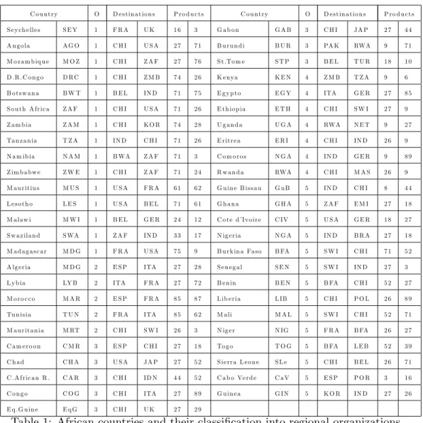
Our approach is applied to a subset of 49 African countries (see Table 1) and from this data source, trade similarities between each pair of countries are used to de…ne networks of links between countries.

Table 1 shows the 49 African countries we have been working with. It also shows the regional organization of each country, accordingly to the following classi…cation: 1 Southern African Development Community (SADC); 2 -União do Magreb Árabe (UMA); 3 - Comunidade Económica dos Estados da Africa Central (CEEAC); 4 - Common Market for Eastern and Southern Africa (COMESA) and 5 - Comunidade Económica dos Estados da África Ocidental (CEDEAO).

For each African country in Table 1, we consider the set of countries to which at least one of the African countries had exported in the year of 2014. The speci…cation of the destinations of exports of each country followed the International Trade Statistics database ([16]) from where justthe …rst and

the second main destinations of exports of each country were taken.

Similarly and also for each African country in Table 1, we took the set of commodities that at least one of the African countries had exported in 2014. The speci…cation of the destinations of exports of each country followed the same database from where just the …rst and the second main export

commodities of each country were taken.

For each country (column label »Country«) in Table 1, besides the regional organization (column label »O«) and the …rst and second desti-nations (column labels »Destinations«) and commodities (column labels

[16]) so that the size of the representation of each country in the networks herein presented is proportional to its corresponding export value in 2014.

C ou ntry O D estin ation s P ro d u cts C ou ntry O D estin ation s P ro d u cts

S ey ch elles S E Y 1 F R A U K 16 3 G ab on G A B 3 C H I JA P 27 44

A n gola AG O 1 C H I U S A 27 71 B u ru n d i B U R 3 PA K RWA 9 71

M ozam b iq u e M O Z 1 C H I Z A F 27 76 S t.Tom e S T P 3 B E L T U R 18 10

D .R .C on go D R C 1 C H I Z M B 74 26 K enya K E N 4 Z M B T Z A 9 6

B otsw an a B W T 1 B E L IN D 71 75 E gy p to E G Y 4 ITA G E R 27 85

S ou th A frica Z A F 1 C H I U S A 71 26 E th iop ia E T H 4 C H I S W I 27 9

Z am b ia Z A M 1 C H I K O R 74 28 U gan d a U G A 4 RWA N E T 9 27

Tan zan ia T Z A 1 IN D C H I 71 26 E ritrea E R I 4 C H I IN D 26 9

N am ib ia N A M 1 B WA Z A F 71 3 C om oros N G A 4 IN D G E R 9 89

Z im b abw e Z W E 1 C H I Z A F 71 24 R w an d a RWA 4 C H I M A S 26 9

M au ritiu s M U S 1 U S A F R A 61 62 G u in e B issau G u B 5 IN D C H I 8 44

L esoth o L E S 1 U S A B E L 71 61 G h an a G H A 5 Z A F E M I 27 18

M alaw i M W I 1 B E L G E R 24 12 C ote d ’Ivoire C IV 5 U S A G E R 18 27

S w azilan d S WA 1 Z A F IN D 33 17 N igeria N G A 5 IN D B R A 27 18

M ad agascar M D G 1 F R A U S A 75 9 B u rk in a Faso B FA 5 S W I C H I 71 52

A lgeria M D G 2 E S P ITA 27 28 S en egal S E N 5 S W I IN D 27 3

L y b ia LY B 2 ITA F R A 27 72 B en in B E N 5 B FA C H I 52 27

M oro cco M A R 2 E S P F R A 85 87 L ib eria L IB 5 C H I P O L 26 89

Tu n isia T U N 2 F R A ITA 85 62 M ali M A L 5 S W I C H I 52 71

M au ritan ia M RT 2 C H I S W I 26 3 N iger N IG 5 F R A B FA 26 27

C am ero on C M R 3 E S P C H I 27 18 Togo T O G 5 B FA L E B 52 39

C h ad C H A 3 U S A JA P 27 52 S ierra L eon e S L e 5 C H I B E L 26 71

C .A frican R . C A R 3 C H I ID N 44 52 C ab o Verd e C aV 5 E S P P O R 3 16

C on go C O G 3 C H I ITA 27 89 G u in ea G IN 5 K O R IN D 27 26

E q .G u in e E q G 3 C H I U K 27 29

Table 1: African countries and their classi…cation into regional organizations, their main exporting commodities and their leading destinations of exports in 2014. Source: International Trade Map (http://www.trademap.org) ([16]).

2.1

The Destinations of Exports

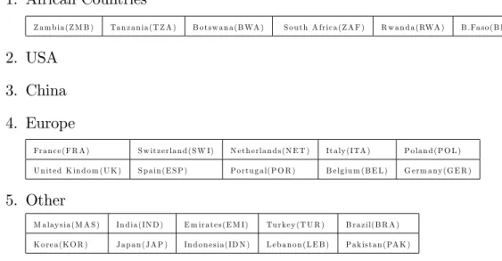
main destinations of exports of each country were taken) are grouped in …ve partition clusters: »African Countries«, »USA, »China«, »Europe«

and »Other«.

1. African Countries

Z am b ia(Z M B ) Tan zan ia(T Z A ) B otsw an a(B WA ) S ou th A frica(Z A F ) R w an d a(RWA ) B .Faso(B FA )

2. USA

3. China

4. Europe

Fran ce(F R A ) S w itzerlan d (S W I) N eth erlan d s(N E T ) Italy (ITA ) Polan d (P O L )

U n ited K in d om (U K ) S p ain (E S P ) Portu gal(P O R ) B elgiu m (B E L ) G erm any (G E R )

5. Other

M alay sia(M A S ) In d ia(IN D ) E m irates(E M I) Tu rkey (T U R ) B razil(B R A )

K orea(K O R ) Jap an (JA P ) In d on esia(ID N ) L eb an on (L E B ) Pak istan (PA K )

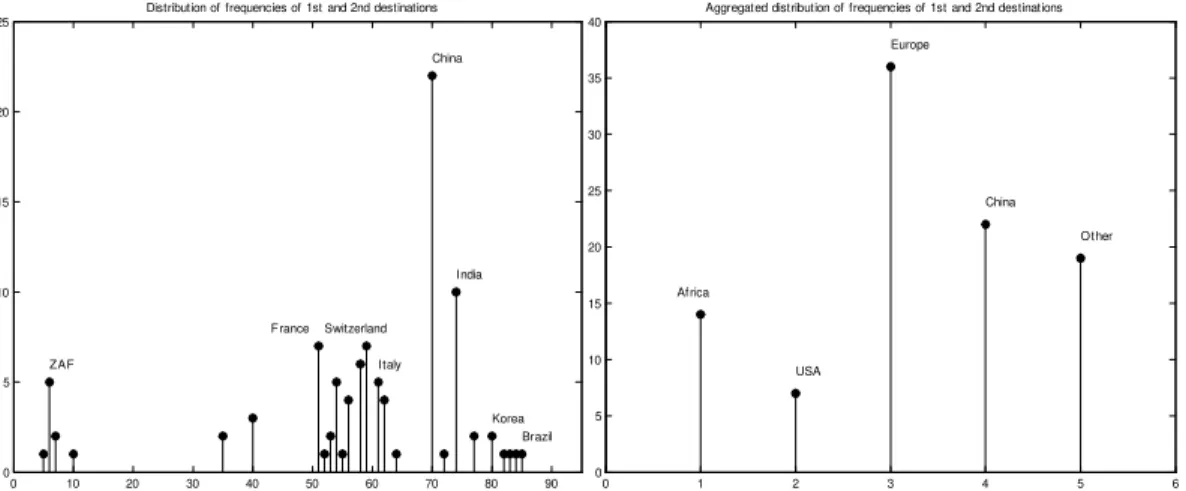
Figure 1 shows the distribution of the frequencies of the two leading destinations of exports of each country in Table 1. The …rst histogram (right) in Figure 1 allows for the observation of the leading destinations of exports from Africa in 2014 and to the way they are distributed by countries. It also shows the distribution of the frequencies (left plot) of the …rst and second destinations when frequencies are aggregated in the …ve partition clusters above described.

0 10 20 30 40 50 60 70 80 90 0 5 10 15 20 25 ZAF China India France Switzerland Italy Brazil Korea Distribution of frequencies of 1st and 2nd destinations

0 1 2 3 4 5 6

0 5 10 15 20 25 30 35 40 Af rica China USA Europe Other Aggregated distribution of frequencies of 1st and 2nd destinations

Figure 1: The distribution of the frequencies of the two leading destinations by country and the same distribution when destinations are aggregated in …ve

partition clusters.

2.2

The Exporting Commodities

The following list of 27 commodities (Commodities14) imported from Africa in 2014 on a …rst and second product basis (as just the …rst and the sec-ond main export commodities of each country were taken) are aggregated in …ve partition clusters: »Petroleum«, »Raw Materials«, »Diamonds«,

»Manufactured Products« and »Other Raw Materials«.

1. Petroleum: HS code: 27(Oil Fuels)

2. Raw Materials (HS code)

03 (… sh ) 06(trees) 08(fru it) 09(co¤ ee) 10(cereals) 16(m eat)

17(su gars) 18(co coa) 24(tob acco) 33(oils) 44(w o o d ) 52(cotton )

3. Diamonds: HS code: 71(Pearls)

4. Manufactured Products (HS code)

28(in org.ch em ic.) 29(org.ch em ic.) 39(p lastics) 61(art.ap p arel) 62(art.ap p arel) 72(iron -steel)

74(cop p er) 75(n ickel) 76(A lu m in iu m ) 85(electricals) 87(veh icles) 89(b oats)

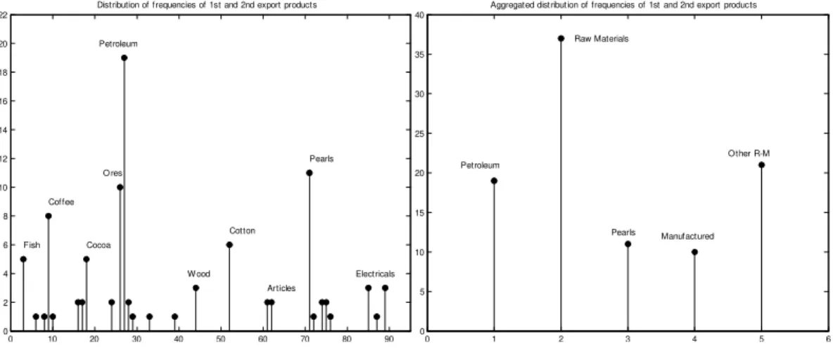
Figure 2 shows the distribution of the frequencies of the two leading export products of each country in Table 1. The second plot (left) shows the same distribution when the products are aggregated according to the …ve partitions of commodities above presented.

0 10 20 30 40 50 60 70 80 90 0 2 4 6 8 10 12 14 16 18 20 22 Petroleum W ood Cotton Cocoa Electricals Pearls O res Fish Coffee Articles Distribution of frequencies of 1st and 2nd export products

0 1 2 3 4 5 6

0 5 10 15 20 25 30 35 40 Petroleum Raw Materials Pearls Manufactured Other R-M Aggregated dist ribution of frequencies of 1st and 2nd export products

Figure 2: The distribution of the frequencies of the two leading export commodities by country and the same distribution when commodities are

aggregated in …ve partition clusters.

From the …rst histogram in Figure 2, one is able to observe the most requested products exported from Africa in 2014 and to the way their fre-quencies are distributed. Not surprisingly, Petroleum crude holds the high-est frequency, being followed by Pearls, Ores and by Co¤ee. The top-…ve exporting commodities in 2014 when frequencies are aggregated are »Raw Materials«, and »Other Raw Materials«, with which »Petroleum« shares a similar frequency.

3

Methodology

Network-based approaches are nowadays quite common in the analysis of systems where a network representation intuitively emerges. It often happens in the study of international trade networks.

ways in which the elementary units and the links between them are de…ned. Here we de…ne two independent bipartite networks where trade similarities between each pair of countries are used to de…ne the existence of every link in each of those networks.

In this section, we analyze the projections of those bipartite networks, the earlier described DSN14 and CSN14 networks are weighted graphs and the weight of each link corresponds to the intensity of the similarity between the linked pair of countries. In the next section, the weighted networks are further analyzed through the construction of their corresponding minimal spanning tress (MST). In so doing, we are able to emphasize the main topological patterns that emerge from the network representations and to discuss their interpretation in the international trade setting.

3.1

Bipartite Graphs

A bipartite network B consists of two partitions of nodes V and W, such that edges connect nodes from di¤erent partitions, but never those in the same partition. A one-mode projection of such a bipartite network ontoV is a network consisting of the nodes in V; two nodes v and v0 are connected in

the one-mode projection, if and only if there exist a node w2 W such that

(v; w) and (v0; w)are edges in the corresponding bipartite network (B). In the following, we explore two bipartite networks and their correspond-ing one-mode projections, the earlier described DSN14 and CSN14 networks.

3.1.1 Topological Coe¢cients

The adoption of a network approach provides well-known notions of graph theory to fully characterize the structure of the projections DSN14and CSN14. These notions are formally de…ned as topological coe¢cients. Here, we con-centrate on the calculation of …ve coe¢cients. Three of them are quantities related to averages values of one topological coe¢cient de…ned at the node level, as the network degree hki, the betweenness centrality hBi and the

av-erage clustering coe¢cient hCi. The other two coe¢cients are measured at the network level, they are the density (d) of the network and the network diameter (D).

1. the average degree (hki) of a network measures the average number of

2. the betweenness centrality (hBi) measured as the fraction of paths con-necting all pairs of nodes and containing the node of interest (i).

3. the clustering coe¢cient (hCi) measures the average probability that

two nodes having a common neighbor are themselves connected

Ci =

E(vi)

vi(vi 1)

(1)

where E(vi) is the size of the neighbourhood (vi) of the node i and the neighbourhood of i consisting of all nodes adjacent to i.

4. the diameter of the network (hDi) measuring the shortest distance be-tween the two most distant nodes in the network.

5. the density (0 d 1) of the network is the ratio of the number of

links in the network to the number of possible links

d= 2L

n(n 1) (2)

whereL is the number of links and n is the number of nodes.

Here, these coe¢cients are computed for di¤erent sub-graphs of both the DSN14 and the CSN14. The nodes (countries) in each sub-graph are grouped accordingly to the partition clusters of main destinations (»African Countries«, »USA, »China«, »Europe« and »Other«) and by partition of main exporting commodity (»Petroleum«, »Raw Materials«, »Diamonds«, »Manufactured Products« and »Other Raw Materials«). We also apply these measures to the partition clusters de…ned by the regional organiza-tions to which the countries belong (SADC, UMA, CEEAC, COMESA and CEDEAO). In so doing, it is possible to compare in terms of topological co-e¢cients the di¤erent structures of the DSN14 and the CSN14networks. For each of them, the topological coe¢cients are computed at the node level and then averaged by partitions of interest (main destination, main commodity or regional organization).

3.2

First Results

3.2.1 Connecting countries by a mutual export destination

The bipartite network DSN14 consists of the following partitions: the set A of 49 African countries presented in Table 1 and

the set of Countries14(Section 2.1) to which at least one of the countries inAhad exported in 2014 on a …rst and second main destination basis. As such, in the DSN14 two countries are linked if and only if they shared a mutual destination of exports in 2014 among their two main export des-tinations. We have considered the two main destinations of exports of each country in Table 1 (columns »Destinations«). Otherwise, if just the main destination was considered, the resulting DSN14 would comprise a set of dis-connected and complete sub-graphs as, by de…nition, each country has just one main destination. Therefore, links in the DSN14 are weighted by the number of coincident destinations a pair of countries share (among the two main destinations of each country in the pair), consequently, every link L(i;j) in the DSN14 takes value in the setf0;1;2g.

As an example, L_(AGO;ZAF) = 2 since AGO and ZAF share two main

destinations of exports in 2014: China and USA.

Another example isL(CM R;CAV)= 1 due to CMR and CaV mutual desti-nation of exports to ESP in 2014.

Among the many examples of missing links there are the cases of AGO and KEN (L(AGO;KEN) = 0) and AGO and CaV (L(AGO;CAV) = 0) since neither AGO and KEN nor AGO and CaV share any mutual leading destination of exports in 2014.

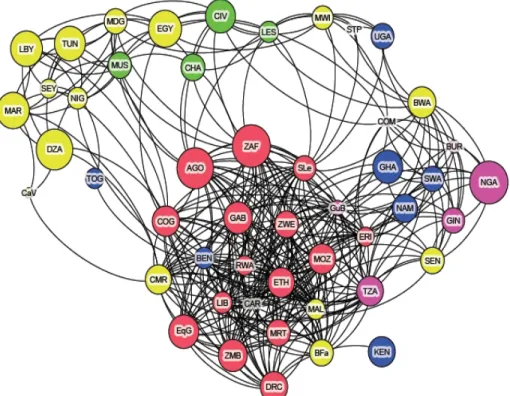
Figure 3 presents the DSN14, a network of 49 African countries linked by mutual leading destinations of exports in 2014. Nodes are colored according to the partition cluster to which their main export destination belongs: red nodes identify countries whose main export destination is »China«, yellow for »Europe«, green for »USA«, blue for »African countries« and purple for the cluster of »Other«.

Such a partition of the set of countries into …ve clusters - de…ned by the country main destination of exports - allows for computing the average values of some topological coe¢cients by partition cluster.

Figure 3: The DSN14colored by partition of main destination.

In all networks presented in this paper, the size of each node is propor-tional to the export value of the country in 2014. Therefore, the largest nodes are ZAF, AGO, DZA and NGA since these countries hold the largest amounts of export values in 2014. Figure 3 shows that the highest connected nodes are those whose main export destination is »China« (colored red), showing that these countries are those that share (with other countries in the whole network) the highest numbers of mutual destinations of exports. On the other hand, there are countries like TOG and STP that share very few mutual destinations with any other countries in the network.

being followed by those that export mainly to countries in the partition of »Other« (colored blue) like TOG and STP.

Another evidence coming out from the network in Figure 3 is that, exclud-ing NGA, the strongest connected countries coincide with the countries with the highest amounts of export values in 2014 (the larger nodes). Not sur-prisingly, it shows a positive non-negligible correlation between the amount of exports of a country and its weighted degree in the DSN14: the countries with the highest amounts of exports in 2014 tend to be those that cluster as exporters to the most frequent African export destinations: »China« and »Europe« (most of the large nodes are yellow and red nodes).

Table 2 shows some topological coe¢cients computed for each node of the DSN14 and averaged by partition of main destination. The second column (»Size«) shows the number of countries in each partition. The averages of the weighted degree (hki), betweenness (hBi) and clustering (hCi) of each

partition show that there is a remarkable clustering in the »China« partition and that although the »Europe« cluster has the same number of nodes, its values of hki;hBi and mostly hCi are far below those of the »China«

partition, con…rming the relevance of the partition of »China« exporters as the very …rst pattern coming out from our approach.

Partition Size hki hBi hCi

Af rica 7 15:8 22:3 0:78

U SA 4 11:6 12:4 0:73

Europe 16 19:4 27:4 0:73

China 16 25:5 32:1 0:96

Other 6 14:5 17:5 0:68

Table 2: The DSN14topological coe¢cients averaged by partition of main destination.

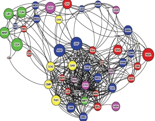
To have an idea on the in‡uence of regional concerns in the patterns that come out in the DSN14, Figure 4 shows the same network of Figure 3 but now the colors of the nodes are de…ned by their regional organizations: blue for SADC countries, green for UMA, yellow for countries in the CEEAC, red for those in COMESA and purple for the countries in CEDEAO.

CEDEAO (red) countries. Together with UMA countries (green) they are the fewest connected countries in the entire DSN14.

Figure 4: The DSN14colored by partition of regional organization.

Table 3 shows some topological coe¢cients computed for each node of the DSN14 and averaged by partition of regional organization. The averages of the weighted degree (hki), betweenness (hBi) and clustering (hCi) of each

partition show that although CEEAC partition (yellow) has just 8 countries, these countries have the greatest centrality (hki and hBi) and clustering in the whole DSN14. This is certainly due to the fact that half of CEEAC countries has »China« as their main export destination and that besides exporting to China, the exports of CEEAC countries are concentrated in a small number of other destinations.

3 and 4. In contrast, UMA countries display low betweenness centrality, showing that besides having »Europe« as their main export destination, the second destination of exports of UMA countries is spread over several countries.

Partition Size hki hBi hCi

SADC 15 17:2 26:7 0:7

U M A 5 12:2 6:5 0:65

CEEAC 8 17 25:9 0:86

COM ESA 7 14:5 13 0:62

CEDEAO 14 14:8 16:6 0:83

Table 3: The DSN14 topological coe¢cients averaged by partition of regional organization.

3.2.2 Connecting countries by a mutual export commodity

Here we develop the commodity share network (CSN14) where African coun-tries in Table 1 are the network nodes and the intensity of a link between each pair of them depends on the number of commodities that they share as export products in 2014.

The bipartite network CSN14 consists of the following partitions:

the set A of 49 African countries presented in Table 1 and

The set of commodities Commodities14 (Section 2.2) that at least one of the countries in the …rst partition have exported in 2014 on a …rst and second commodity basis.

Therefore, in the CSN14two countries are linked if and only if they shared a mutual leading export commodity in 2014. We have considered the two main export products of each country in Table 1 (columns »Products«). Otherwise, if just the main product was considered, the resulting CSN14 would comprise a set of disconnected sub-graphs as each country has just one main exporting product. Links in the CSN14 are weighted by the number of coincident products a pair of countries share (among the two main products), consequently, every link L_(i;j) in CSN₁₄ takes value in the set f0;1;2g.

As an example, the intensity of the link between KEN and UGA equals two (L_{(KEN;U GA)} = 2) since KEN and UGA share two mutual leading

L(ERI;RW A) = 1 due to ERI and RWA mutual leading exports of Ores in 2014. Among the many examples of missing links there are the cases of MOZ and KEN (L_{(M OZ;KEN)} = 0) since MOZ and KEN did not share any

mutual leading export product in 2014.

Figure 5 presents the CSN14, a network of 49 African countries linked by at least one mutual leading export commodity in 2014. Nodes are colored accordingly to the partition cluster to which their main exporting product belongs: blue nodes have »Petroleum« as the main export commodity in 2014, red nodes identify countries whose main export products are »Manu-factured«, yellow for »Diamonds«, green for »Raw Materials« and purple for the cluster of »Other Raw Materials«.

Similarly to what was done within the DSN14, the partition of the set of countries into …ve clusters by main export commodity allows for computing the average values of some topological coe¢cients by partition cluster. In so doing it is possible to compare important patterns coming out from the CSN14. Like in the DSN14 representations, the size of each node is propor-tional to the export value of the country in 2014.

Likewise observed in the DSN14, the graph in Figure 5 suggests the ex-istence of a positive and strong correlation between the amount of exports of a country and its weighted degree in the CSN14: the countries with the highest amounts of exports in 2014 (the larger nodes) tend to be those that cluster as petroleum exporters (blue), being followed by those that export »Diamonds« (yellow) and »Manufactured« (red).

The highest degrees belong to AGO, NGA and ZAF, showing that these countries are those that share (with other countries in the whole network) the highest numbers of mutual export commodities. On the other hand, there are countries like MWI and SWA that share just one exporting commodity with the all other countries in the network.

Figure 5: The CSN14 colored by partition of main export commodity.

Table 4 shows some topological coe¢cients computed for each node of the CSN14 and averaged by partition of main exporting product. The aver-ages of the weighted degree (hki), betweenness (hBi) and clustering (hCi) of each partition show that the strongest connected countries are those whose main exporting product is »Petroleum«. In terms of connectivity, they are followed by the cluster of Manufactured Products, even though this cluster has just six countries.

There is a very high value of betweenness centrality (hBi)

Partition Size hki hBi hCi

P etroleum 15 21:6 35:5 0:82

RawM aterials 15 9:9 14:1 0:72

Diamonds 7 14:2 33:7 0:70

M anuf actured 6 18:6 22:3 0:77

OtherRM 6 4:5 5:8 0:48

Table 4: The CSN14 topological coe¢cients averaged by partition of main exporting product.

Another interesting characteristic is the poor connectivity pattern of countries in the »Raw Materials« partition cluster. Even being a large par-tition in size, its average weighed degree (hki) is the second smallest in the

CSN14. It means that countries that mainly export raw materials have a small share of mutual export products with other countries.

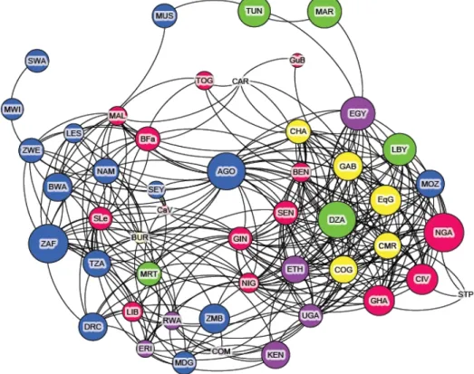
Figure 6: The CSN14 colored by partition of regional organization.

regional organizations: blue for SADC countries, green for UMA, yellow for countries in the CEEAC, red for those in COMESA and purple for the countries in CEDEAO.

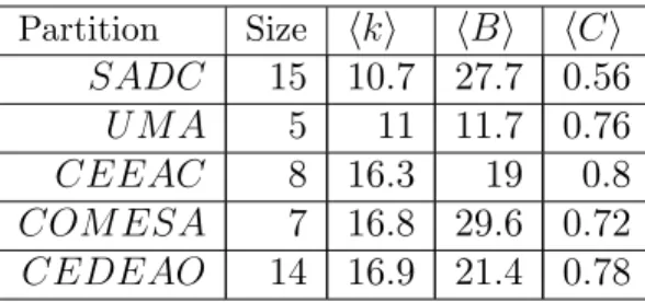
Table 5 shows some topological coe¢cients computed for each node of the CSN14 and averaged by partition of regional organization. There, the CEEAC partition (yellow) although having just eight countries, has the great-est clustering (hCi) in the whole CSN14. On the contrary, the SADC cluster, although comprising a large number of countries, is the one of the poorest clustering value in the ranking of …ve partitions presented in Table 5.

Another evidence coming out from the regional perspective is that with-out AGO and MOZ, the large set of …fteen SADC countries (blue) would be excluded from the large cluster of »Petroleum« exporters. This is certainly related to the small clustering that SADC countries have in the CSN14, being most of SADC countries mainly diamond and ore exporters.

Partition Size hki hBi hCi

SADC 15 10:7 27:7 0:56

U M A 5 11 11:7 0:76

CEEAC 8 16:3 19 0:8

COM ESA 7 16:8 29:6 0:72

CEDEAO 14 16:9 21:4 0:78

Table 5: The CSN14 topological coe¢cients averaged by partition of regional organization.

3.2.3 Comparing the destination share and the commodity share

networks

Table 6 shows some network coe¢cients computed for the DSN14 and the CSN14. The coe¢cients hki, hBi and hCi were computed at the node level and averaged by network. The averages of the weighted degree (hki),

be-tweenness (hBi) and clustering (hCi) of these networks show that for the 49

African countries in 2014, sharing a mutual leading export product happens less often than sharing a mutual leading destination of exports, since the degree of the DSN14 is greater than the degree of the CSN14.

the CSN14 is larger than the diameter of the DSN14, the 49 African coun-tries are on average closer to each other when connected by a mutual leading export destination than when connected by a mutual exporting product.

Graph Size hki hBi hCi density diameter DSN14 49 15:6 19:7 0:76 0:31 3 CSN14 49 14:3 23:1 0:72 0:28 5

Table 6: Comparing topological coe¢cients obtained for DSN14and CSN14.

The DSN14 also has a larger clustering coe¢cient than the CSN14, show-ing that when a country shares a mutual export destination with other two countries, these two other countries also tend to share a mutual export des-tination between them. The densities of DSN14 and CSN14 con…rm that topological distances in the DSN14 are shorter than in the CSN14 and that on average going from one country in the DSN14 to any other country in the same graph takes less intermediate nodes than in the CSN14.

Although the networks DSN14 and CSN14 inform about the degree of the nodes, their densely-connected nature does not help to discover any dominant topological pattern besides the distribution of the node’s degree. Moving away from a dense to a sparse representation of a network, one shall ensure that the degree of sparseness is determined endogenously, instead of by an a priory speci…cation. It has been often accomplished ([17],[18]) through the construction of a Minimal Spanning Tree (MST), in so doing one is able to develop the corresponding representation of the network where sparseness replaces denseness in a suitable way.

3.3

The Minimum Spanning Tree Approach

In the construction of a MST by the nearest neighbor method, one de…nes the 49 countries (in Table 1) as the nodes (Ni) of a weighted network where the distance dij between each pair of countries i and j corresponds to the inverse of weight of the link (dij = _L1

ij) between i and j.

From the N xN distance matrix D, a hierarchical clustering is then per-formed using thenearest neighbor method. InitiallyN clusters corresponding to theN countries are considered. Then, at each step, two clustersci and cj are clumped into a single cluster if

with the distance between clusters being de…ned by

dfci; cjg= minfdpqg with p2ci and q 2cj (4)

This process is continued until there is a single cluster. This clustering process is also known as the single link method, being the method by which one obtains the minimal spanning tree (MST) of a graph.

In a connected graph, the MST is a tree of N 1 edges that minimizes

the sum of the edge distances. In a network with N nodes, the hierarchical clustering process takesN 1steps to be completed, and uses, at each step, a particular distance di;j 2D to clump two clusters into a single one.

4

Results

In this section we discuss the results obtained from the MST of each one-mode projected graphs DSN14 and CSN14. As earlier mentioned, the MST of a graph may allow for discovering relevant topological patterns that are not easily observed in the dense original networks. As in the last section, we begin with the analysis of the DSN14 and then proceed to the CSN14.

We look for eventual topological structures coming out from empirical data of African exports, in order to see whether some relevant characteristics of African trade have any bearing on the network structures that emerge from the application of our approach. In the last section, we observed some slight in‡uence of the regional position of each country in its connectivity. With the construction of the minimum spanning trees we envision that some stronger structural patterns would come to be observed on the trees.

4.1

The MST of the destination share network

Figure 7 shows the MST obtained from the DSN14 and colored according to each country main destination of exports in 2014.

Interestingly, the countries that exports to »African countries« (blue) occupy the less central positions on the tree. This result illustrates the suitability of the MST to separate groups of African countries according to their main export destinations and the show how opposite are the situations of those that export to »China« from the countries that have Africa itself as their main export destinations.

Figure 7: The MST of the CSN14 colored by partition of main destination.

4.2

The MST of the commodity share network

Figure 8 shows the MST obtained from the CSN14 and colored according to the main export commodity of each country in 2014. The …rst observation on the MST presented in Figure 8 is that, centrality is concentrated in a fewer number of countries (when compared to the MST of the DSN14).

Figure 8: The MST of the CSN14 colored by partition of main exporting commodity.

The top most central and connected positions are shared by countries belonging to two regional organizations: SADC and CEDEAO, being mainly represented by ZAF and AGO and clustering countries whose main export commodities are »Diamonds« and »Petroleum«, respectively. Unsurpris-ingly, centrality and connectivity advantages seem to be concentrated in these two leading commodity partitions (»Diamonds« and »Petroleum«) and organization groups (SADC and CEDEAO).

the leaf positions, being weakly connected to the other African countries to which, the few connections they establish rely on having »Manufactured« as their main export commodity. Likewise, there is a branch clustering exporters of »Raw Materials« (green) being also placed at the leaf positions on the tree. Such a lack of centrality of »Raw Materials« exporters in the CSN14 seems to be due to the fact that their leading export products are spread over many di¤erent commodities (the »Raw Materials« partition comprises 12 di¤erent commodities).

5

Concluding remarks

In the last decade, a debate has taken place in the network literature about the application of network approaches to model international trade. In this context, and even though recent research suggests that African countries are among those to which exports can be a vehicle for poverty reduction, these countries have been insu¢ciently analyzed.

We have proposed the de…nition of trade networks where each bilateral relation between two African countries is de…ned from the relations each of these countries hold with another entity. Both networks were de…ned from empirical data reported for 2014.They are independent bipartite networks: a destination share network (DSN14) and a commodity share network (CSN14). In the former, two African countries are linked if they share a mutual leading destination of exports, and in the latter, countries are linked through the existence of a mutual leading export commodity between them.

Our conclusions can be summarized in the following.

1. Sharing a mutual export destination happens more often: The very …rst remark coming out from the observation of both the DSN14 and the CSN14 is that, in 2014 and for the 49 African countries, sharing a mutual exporting product happens less often than sharing a mutual destination of exports.

exploration ([7],[8],[9],[10], [11],[12],[13]) and the one that speci…cally focus on African trade ([1],[2],[3],[4],[5],[6]). References ([2],[4]) reports on the role of export performance to economic growth. They also dis-cuss on the relation between trade and development, and on the growth by destination hypothesis, according to which, the destination of ex-ports can play an important role in determining the trade pattern of a country and its development path.

3. Destination matters: The idea that destination matters is in line with our …nding that in the DSN14, the highest connected nodes are those whose main export destination is China. According to Baliamoune-Lutz ([4]) export concentration enhances the growth e¤ects of exporting to China, implying that countries which export one major commodity to China bene…t more (in terms of growth) than do countries that have more diversi…ed exports.

The China e¤ect: One of the patterns that came out from our DSN14 shows that half of CEEAC and SADC countries belongs to the bulk of »China« destination cluster, having high between-ness centrality. Additionally, the »China« destination group of countries displays the highest clustering coe¢cient (0.96), mean-ing that, besides havmean-ing China as their main exports destination, the second destination of exports of the countries in this group is highly concentrated on a few countries.

The Angola cluster: our results highlighted the remarkable cen-trality of AGO as the center of the most central cluster of »China« exporters. Indeed, AGO is the country that holds the most cen-tral position when both DSN14 and CSN14 are considered. This country occupies in both cases the center of the largest central clusters: »China« exporters in DSN14 and exporters of »Petro-leum« in CSN14.

UMA countries anti-diversi…cation: In the opposite situation, we found that UMA countries display very low centrality, showing that besides having »Europe« as their …rst export destination, the second destination of exports of UMA countries is spread over several countries. This result is in line with reference ([6]) report on European unilateral trade preferences and anti-diversi…cation e¤ects. We showed that UMA countries occupy a separate branch in the MST of the DSN14, being »Europe« their most frequent destination of exports.

4. In the CSN14, the highest connected nodes are those that cluster as »Petroleum« exporters, being followed by those that export »Dia-monds«. Unsurprisingly, »Raw Materials« exporters display very low connectivity as their second main exporting product is spread over sev-eral di¤erent commodities.

5. Organizations matter: Regional and organizational concerns seem to have some impact in the CSN14.

SADC and Petroleum: The group of SADC countries, although comprising a large number of elements, is the one with the poorest connectivity and clustering in the CSN14. It is certainly due to the fact that without AGO and MOZ, this large group of countries does not comprise »Petroleum« exporters.

-were shown to characterize countries that export mainly to »Eu-rope« and whose main exporting product is »Raw Materials«.

Future work is planned to be twofold. We plan to further improve the de…nition of networks of African countries, enlarging the set of similarities that de…ne the links between countries in order to include aspects like mother language, currencies, demography and participation in trade agreements. On the other hand, we also plan to apply our approach to di¤erent time periods. As soon as we can relate the structural similarities (or di¤erences) and their evolution in time to certain trade characteristics, the resulting knowledge shall open new and interesting questions for future research on African trade.

References

[1] Portugal-Perez, A. and Wilson, J.S. (2008) Trade Costs in Africa: Bar-riers and Opportunities for Reform, in Policy Research Working Paper 4619.

[2] Kamuganga, Dick N. (2012) What drives Africa‘s export diversi…ca-tion?, in Graduate Institute of International and Development Studies Working Paper, No. 15/2012.

[3] Ackah, C. and Morrissey O. (2007) Trade Protection as Income Protec-tion in Poor Countries in GEP-Murphy Institute Conference on New Political Economy of Globalization, New Orleans.

[4] Baliamoune-Lutz, M. (2011) Growth by Destination (Where You Export Matters): Trade with China and Growth in African Countries in African Development Review, Special Issue: Special Issue on the 2010 African Economic Conference on “Setting the Agenda for Africa’s Economic Recovery and Long-term Growth” V.23, 2.

[5] Ackah, C. and Morrissey O. (2005) Trade policy and performance in Sub-Saharan Africa since the 1980s, in School of Economics, University of Nottingham: CREDIT Research Paper 07/01.

Trade Preferences on Intensive and Extensive Margin of Trade, IHEID working paper 17.

[7] Serrano, M.; Boguná, M. and Vespignani, A. (2007) Patterns of domi-nant ‡ows in the trade web, in J. Econ. Interact. Coord., V.2.

[8] Almog, A.; Squartini, T. and Garlaschelli, D. (2015) The Double Role of GDP in Shaping the Structure of the International Trade Network, arXiv:1512.02454.

[9] Fagiolo, G.; Reyes J. and Schiavo S. (2009) World-trade web: Topolog-ical properties, dynamics, and evolution, in Phys. Rev. E, V.79.

[10] Saracco, F.; Di Clemente, R.; Gabrielli, A. and Squartini, T. (2015) De-tecting the bipartite World Trade Web evolution across 2007: a motifs-based analysis, arXiv:1508.03533.

[11] De Benedictis, L.; Tajoli, L. (2011) The world trade network, in The World Economy, V.34.

[12] Picciolo, F.; Squartini, T.; Ruzzenenti, F.; Basosi, R. and Garlaschelli, D. (2012) The role of distances in the World Trade Web,in Proceedings of the Eighth International Conference on Signal-Image Technology & Internet-Based Systems (SITIS 2012).

[13] Yang, Y; Poonb, J., Liua, Y. and Bagchi-Senb, S. (2015) Small and ‡at worlds: A complex network analysis of international trade in crude oil, in Energy (Elsevier) V.93.

[14] Bergstrand, J. (1985) The Gravity Equation in International Trade: some Microeconomic, Foundations and Empirical Evidence, in Review of Economics and Statistics, V. 67, 3.

[15] Araújo. T. and Banisch, S. (2014), Multidimensional Analysis of Lin-guistic Networks,in Towards a Theory of Complex Linguistic Networks, Springer, Berlin.

[16] International Trade Map (http://www.trademap.org).