Applications residual control charts based on variable limits

A Mendonça Souza et al. Int. Journal of Engineering Research and Applications www.ijera.com

ISSN : 2248-9622, Vol. 5, Issue 5, ( Part -1) May 2015, pp.44-50

Applications Residual Control Charts Based on Variable Limits

Adriano Mendonça Souza*, Francisca Mendonça Souza**, Roselaine Ruviaro

Zanini***, Bianca Reichert****, Afonso Valau De Lima Junior*****

*(Industrial Engineering Post-graduation Program, Federal University of Santa Maria – UFSM, Brazil) ** (Department of Quantitative Methods, ISCTE Business School - Lisbon University Institute, Portugal) ***(Industrial Engineering Post-graduation Program, Federal University of Santa Maria – UFSM, Brazil) ****(Industrial Engineering Graduate Student, Federal University of Santa Maria – UFSM, Brazil)

*****( Industrial Engineering Post-graduation Program, Federal University of Santa Maria – UFSM, Brazil)

ABSTRACT

The main purpose of this paper is to verify the stability of a productive process in the presence of the effects of autocorrelation and volatility, in order to capture these characteristics by a joint forecast model which produces residuals that are evaluated by a control chart based on variable control limits. The methodology employed will be the joint estimation of the residuals by ARIMA – ARCH models and the conditional standard deviation from residuals to establish the chart control limits. The joint AR (1)-ARCH (1) model shows that an appropriate forecasting model brings a great contribution to the performance of residual control charts in monitoring the stability of industrial variables using just one chart to monitor mean and variance together.

Keywords

- ARCH models, ARIMA models, Autocorrelated data, Statistical process control, Volatility in industrial processes.

I. INTRODUCTION

Statistical Process Control uses statistical techniques to meet the quality of conformance [1]. Control charts were developed by Walter A. Shewhart in 1924 [2] and are the simplest tool to monitor a productive process. But, in order to apply this kind of charts, some assumptions are necessary to get more accuracy and chart interpretability: the sample data to be analyzed must follow the Normal distribution and be independent and identically distributed (i.i.d.) [3], [4], [5], [6], [7].

In many industrial cases data are correlated, so the assumptions about control charts are not satisfied. An alternative to this problem is to fit an autoregressive integrated moving average (ARIMA) model and then apply the appropriated control chart on the residuals of the ARIMA model [8], evaluating the process stability this way [9].

When an ARIMA model is fitted, the residuals must follow a withe noise condition that is being not autocorrelated, homoskedastic and follow the Normal Distribution. If the residuals do not meet these conditions, the model could be considered poor or not efficient to explain and forecast the series.

However, as noted by several authors such as [10], [11], [12], [13], the residuals of a linear model may be conditionally heteroskedastic, that means that the residuals can show some kind of dependency. This dependency of the residuals can be investigated by an autoregressive conditional heteroskedasticity model (ARCH). The ARCH models proposed by [14] and [15] explain volatility using the past squared

residual values originated from a linear prediction model. Considering that the variance is not constant over the time, [10] if these characteristics are neglected, there are consequences in terms of the quality of the parameter estimation and, consequently, in the forecasting values and residuals. Thus, linear models (ARIMA) are used to capture these effects in relation to the mean process and nonlinear models (ARCH) are used to understand the variance behavior.

In terms of control charts, used to monitor autocorrelated process, these two information about the productive processes must be considered - mean and volatility behavior. Therefore, the main purpose of this paper is to establish residual control charts based on variable control limits in the presence of volatility, which incorporates the variability to set the control limits.

Due to the importance of forecasting models, this study also aimed to show the application of new modeling tools that can help in the evaluation of statistical process control methodology in order to follow the technological advances.

The characteristics of autocorrelation and heteroskedasticity in variables that come from chemical processes, such as viscosity, pressure and temperature, may show autocorrelated and heteroskedasticity characteristics, and this characteristics, in general, violate the initial assumptions to apply control charts.

The main objective of a control chart is to monitor a quality characteristic, but sometimes the

A Mendonça Souza et al. Int. Journal of Engineering Research and Applications www.ijera.com

ISSN : 2248-9622, Vol. 5, Issue 5, ( Part -1) May 2015, pp.44-50

variable of interest is autocorrelated, requiring some alternatives to accomplish the control charts assumptions.

The most common alternative is to fit an autoregressive integrated moving average (ARIMA) model and remove serial correlation. So the residual that comes from this model is used to represent the process that is being investigated because a white

noise residual is used. Nevertheless, the constant

variance is not always observed and it is rarely tested for the application in statistical process control. The non-constant variance is called volatility and it is represented by periods of great and low variability, causing a great instability in the process. This volatility is called conditional volatility, represented by a nonlinear autoregressive conditional heteroskedasticity (ARCH) model. To find it, a square residual derivated from a linear model, such as an ARIMA model [11], [12], is used.

In this study we propose to establish a control chart, where the ARIMA residuals model will be used to represent the center line of the chart and the control limits will be based on the conditional variance, so mean and variance will be shown together in just one chart.

II. METHODOLOGY

The methodological steps to be followed in order to obtain a residual series free of autocorrelation and heteroskedasticity to apply the residual control charts are:

Step 1: Fit the linear model - ARIMA (p, d, q), using the B-J methodology [16], [17] in order to remove serial correlation and analyze the series residuals. Autoregressive and integrated moving average (ARIMA) models are based on the theory that the behavior of the variable itself answers for its future dynamics [17]. Generally, a non-stationary process follows an ARIMA (p, d, q) process, as in (1).

(1) where, B is the retroactive operator, d represents the order of integration; ϕ is the term represented by the autoregressive order p, and θ is the moving average parameter represented by q, and et ≈ N(0, σ2), which is white noise.

Authors as [18], [19], [20], [21] and [22] have showed that to elaborate an ARIMA model an iterative cycle should be followed in four steps: model identification; parameter estimation by Maximum Likelihood Estimation (MLE) method; diagnostic test or check and, if the model is adequate, the forecasting is done.

The best model in terms of number of parameters is based on Akaike's Information Criteria (AIC) and Bayesian Information Criteria (BIC), because they consider the number of estimated parameters.

n

SQR

T

AIC



ln(

)



2

₍₂₎

)

ln(

)

ln(

SQR

n

T

T

BIC





₍₃₎

where, T is the sample size; SQR is the sum of the squared residuals, n is the number of parameters.

But it is necessary that the residuals are white noise. After estimating the appropriate ARIMA model, the residual assumption is verified. If the homoscedasticity is not met, it is necessary to choose an ARCH model to estimate the volatility of the residuals.

Step 2: Heteroskedasticity residual analysis in order to verify the presence of autoregressive conditional heteroskedasticity using the ARCH-LM test proposed by [14]. If there is evidence of heteroskedasticity, a nonlinear model - ARCH (p) – is estimated, so the joint modeling is done by ARIMA-ARCH models considering the level and volatility effects of the series [23].

The main idea behind the ARCH model is the fact that the variance et at time t, depends on e2t-1. As the variability can be explained by the volatility that exists in the residuals that come from the linear prediction model, one can observe that the variance of these errors is not constant over time, it varies from one period to another. Thus, there is an autocorrelation in the variance residual forecast [15], [21].

According to [14], [20] and [21] if a residual of a linear process follows an ARCH process, it can be set as in (4), where there is the basic expression of the ARCH model.

(4) It can be observed, this way, that the conditional variance of the error εt to the information available to the period (t-1) would be distributed, and according to [13], there would be the (5).

(5) In the case of an ARCH (1) model, the conditional variance is defined by (6).

(6) Thus, it is expected that ARCH (1) modeling provides a residual with i.i.d. characteristics [24] as shown in (7).

) (7) where, α0 and α1 are the parameters that explain the residual variance term [23].

Step 3: Application of mean control charts for individual measures [25], [26] in data free of autocorrelation and heteroskedasticity effects residuals.

The residual control chart [27] proposed is composed by a central line (CL), formed by the residuals estimated by an ARIMA model in the step 1, which represents the characteristic average value that is controlled or monitored. The upper control

A Mendonça Souza et al. Int. Journal of Engineering Research and Applications www.ijera.com

ISSN : 2248-9622, Vol. 5, Issue 5, ( Part -1) May 2015, pp.44-50

limit (UCL) and lower control limit (LCL) will be estimated at three standard deviations (3σ) from the CL, but the standard deviation will be that one estimated at each new point by means of an ARCH model in step 2. In this way, it is not assumed to find constant variance over the time to ensure stability to the estimated parameters and it can be seen that the variance has a different behavior over the time. In this study, the option is to use X-bar control charts for individual measurements with variable control limits, where the mean and variance will be displayed at the same chart. For the X-bar individual measures, the limits placed at three standard deviations from the mean are given by (8).

(8)

where K is the multiple of standard deviation, K = 0 1, 2, 3, et is the residual estimated by an ARIMA model, and is the variance estimated at each new sample by the ARCH model. It is important to highlight that in the presence of non-independent data, the control charts are not effective in detecting out of control points. Authors such as [28] and [29] suggest using a forecasting model to eliminate the autocorrelation and use the residual from this forecast model to evaluate the process stability. Thus, the model that best explains the variable of interest is the one that best produces residuals able to represent the process and to be

INVESTIGATED BY CONTROL CHARTS.

The performance of control charts is checked by the number of out of control points detected when analyzing the real data and the residual from the ARIMA-ARCH model, that represents the original process.

III. RESULTS

AND

DISCUSSION

This study analyzes the burning and drying stages of tiles ceramic pieces, at the preheating stage with an average temperature around 400ºC. The variable analyzed form a data series with 92 observations, taken in intervals of one hour from each other.

Fig. 1 shows that the preheating variable, which is not stable around the mean, with some extreme points and apparently great variability.

464 468 472 476 480 484 10 20 30 40 50 60 70 80 90 Fig. 1 - Original series of preheating temperature of

drying stage of tiles ceramic pieces

I. Modeling step

The series was considered stationary by the Augmented Dickey Fuller test [30] (tStatistic = -4,5424 and p-value = 0,0003) where the null hypothesis is that preheating has a unit root. To confirm this, the Kwiatkowski-Philipps-Schimidt-Shin test was performed (LM-stat = 0,0695 and

KPSS-statistic = 0,7390), concluding that the series is

stationary. As the data series is stationary, the model AR(1) – ARCH(1) is fitted and shown at Table 1.

Table 1 – Estimation of coefficients, standard-error, Z statistic and p-value of AR-ARCH model to the

acidity index of soybean oil Method: ML – ARCH (Marquardt) Normal distribution

Mean conditional equation

Coeff St. error Z stat

p-value Const AR (1) 476.1778 0.5222 0.5138 0.0630 926.735 8.279 0.000 0.000 Conditional variance equation

Const ARCH(1) 3.6201 0.4372 0.6796 0.2026 5.3263 2.1579 0.000 0.3090 To verify the presence of conditional heteroskedasticity the ARCH-LM test, proposed by Engle [1013], was performed on the residuals obtained from the AR (1) model Table 1.

The model that describes the mean and the volatility is described by a joint AR (1) - ARCH (1) model presenting statistically significant parameters and the residual series behaving as white noise. The model validation was performed by examining statistics such as skewness, kurtosis, as well as normality and residual independence. From model in Table 1 it is possible to show the residuals of preheating temperature.

A Mendonça Souza et al. Int. Journal of Engineering Research and Applications www.ijera.com

ISSN : 2248-9622, Vol. 5, Issue 5, ( Part -1) May 2015, pp.44-50

-10.0 -7.5 -5.0 -2.5 0.0 2.5 5.0 7.5 10.0 10 20 30 40 50 60 70 80 90 PRE1 Residuals

Fig. 2 – Residuals of preheating temperature originated by an AR(1) model

As it was shown the residuals follow a white

noise and they are not autocorrelated, but both the

Breusch-Godfrey serial correlation LM test, with

Fstatistic = 0,016202 and Ftab (2,87) = 0,98, and the

Maximum Likelihood test T= n.R2 = 0,03381, with

X2(2) = 0,98, show no evidence to accept

homoskedastic residuals.

The conditional standard deviation in Fig. 3 shows the volatility present in the data analyzed.

1 2 3 4 5 6 7 10 20 30 40 50 60 70 80 90

Conditional standard deviation

Fig. 3 – Conditional standard deviation on the residuals of preheating temperature established by

an ARCH(1) model.

It is possible to notice that most of time the volatility is almost constant, but there are periods of high volatility around 20, 35 and 45 periods. This variability can affect the control limits that can be wider due to instability present in data. The ARCH (1) parameter estimated value of 0.4372 shows that this behavior is not lasting for a long time and the variability will return to its regular movement.

II. Process stability analysis

The process stability analysis at this moment is represented by the X-bar chart for individual measurements. The difference in the control chart proposed is that mean and variability will be analyzed together, because the center line will be represented by the ARIMA residuals and the control

limits variability by the standard deviation estimated by the ARCH model. So, the control limits will be variable.

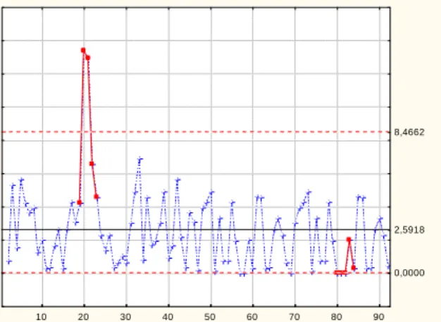
In Fig. 4, the control limit chart was set up with 2-standard deviations from the center line, and it is important to observe that there are points out of the control limits. Possibly due to high volatility present in data and reveled by the residuals series.

Fig. 4 – Residual control chart for individual measurements of preheating temperature using variable control limits at 2-standard deviations

In Fig. 5, the control limits were set up based on 3–standard deviations, and even so the high distance from the center line showed in the original data, around the observation 20nd, was detected.

Fig. 5 – Residual control chart for individual measurements of preheating temperature using variable control limits at 3- standard deviations

Fig. 4 and 5 showed that the joint AR (1) – ARCH (1) model to monitor residuals is able to detect points out of the control limits.

As a way to compare the performance of residual control charts with variable limits, the regular residual control chart for individual measurements and for moving range were established at 2-standard deviations from the center line, as shown in Fig. 6 and 7 respectively.

A Mendonça Souza et al. Int. Journal of Engineering Research and Applications www.ijera.com

ISSN : 2248-9622, Vol. 5, Issue 5, ( Part -1) May 2015, pp.44-50

10 20 30 40 50 60 70 80 90

0,0000 2,5918 8,4662

Fig. 6 – Residual control chart for individual measurements of preheating temperature using

control limits at 2-standard deviations

10 20 30 40 50 60 70 80 90

0,0000 2,5918 8,4662

Fig. 7 – Residual control chart for moving range for individual measurements of preheating temperature

using control limits at 2-standard deviations To another comparison, 3-standard deviations from the center line residual control chart for individual measurements and for moving range were established as shown in Fig. 8 and 9 respectively.

It is important to highlight that if control charts were applied directly on the original variable, the assumptions imposed by Shewhart control charts would have been violated. On the other hand, using the joint AR (1) - ARCH (1) model [31], it was possible to capture the mean and variability behavior in just one model and show them in just on control chart. It is also important to notice that the variable control limits were able to follow the residuals movement without detecting points out of control, just compare Fig. 4 with Fig. 6 and Fig. 7, where control limits were established at 2-standard deviations. And, at 3-standard deviations, compare Fig. 3, with Fig. 8 and Fig. 9.

10 20 30 40 50 60 70 80 90

-6,8908 -0,4E-12 6,8908

Fig. 8 – Residual control chart for individual measurements of preheating temperature using

control limits at 3-standard deviations

10 20 30 40 50 60 70 80 90

0,0000 2,5918 8,4662

Fig. 9 – Residual control chart for moving range for individual measurements of preheating temperature

using control limits at 3-standard deviations

IV. CONCLUSIONS

The joint AR (1)-ARCH (1) model shows that an appropriate forecasting model brings a great contribution to the performance of residual control charts in monitoring the stability of industrial variables.

The relevance of this study is to present an alternative approach to traditional techniques of statistical process control. The volatility, that was a problem in industrial process, has, nowadays, a great contribution in making it possible to determine the variability at each sample that is produced, by means of ARCH models.

A residual control chart is expected to behave as

white noise and be not autocorrelated, but some kind

of dependency was found – ARCH (1) – and it was useful to establish variable control limits at each sub sample plotted in the control chart.

As a new research, it is recommended to conduct a study with simulated data to study the performance of this methodology with other models and its efficiency using the average runs lengths (ARL).

A Mendonça Souza et al. Int. Journal of Engineering Research and Applications www.ijera.com

ISSN : 2248-9622, Vol. 5, Issue 5, ( Part -1) May 2015, pp.44-50

Acknowledgements

The first and second authors thanks to the financial support of Foundation, Ministry of Education of Brazil - CAPES – Process grants nº BEX-1784/09-9- CAPES – and nº BEX- 5416/10-8 – CAPES, and ISCTE Business School - Lisbon University Institute. And all of them thanks to the Analysis and Modeling Statistics Laboratory at Federal University of Santa Maria – UFSM.

R

EFERENCES

Journal Papers:

[1] O. Rama MohanaRao, .VenkataSubbaiah, K.NarayanaRao, T. Srinivasa Rao. Application of Univariate Statistical Process Control Charts for Improvement of Hot Metal Quality- A Case Study. International

Journal of Engineering Research and Applications (IJERA). Vol. 3, Issue 3, May-Jun 2013, pp.635-641.

[3] Mingoti, S. A.; Yassukawa, F. R. S., Uma comparação de gráficos de controle para a média de processos autocorrelacionados.

Revista Eletrônica Sistemas & Gestão, v.3, n. 1, p. 55-73, jan-abr. 2008.

[4] Silva, W. V.; Fontanini, C. A. C.; Del Corso, J. M., Garantia da qualidade do café solúvel com o uso do gráfico de controle de somas acumuladas. Revista Produção on-line, v. 7,

n. 2, p. 43-63, 2007.

[5] Claro, F. A. E.; Costa, A. F. B.; Machado, M. A. G., Gráficos de controle de EWMA e de X-barra para monitoramento de processos autocorrelacionados. Revista Produção, v.

17, n. 3, p. 536-546, set-dez. 2007.

[6] Ramos, A. W.; Ho, L. L., Procedimentos inferenciais em índices de capacidade para dados autocorrelacionados via bootstrap.

Revista Produção, v. 13, n. 3, p. 50-62,

2003.

[7] Souza, A. M.; Samohyl, R. W.; Malavé, C. O., Multivariate feedback control: an application in a productive process.

Computers & Industrial Engineering, v. 46, p. 837-850, 2004.

[8] N.A. Bhatia and T.M.V.Suryanarayana. Study of Time Series and Development of System Identification Model for Agarwada Raingauge Station. International Journal of

Engineering Research and Applications. Vol. 1, Issue 3, pp.1072-1079.

[9] Vanusa Andrea Casarin1, Adriano Mendonça Souza, Rui Menezes3, Jaime Alvares Spim. Continuous Casting Process Stability Evaluated by means of Residuals Control Charts in the Presence of Cross-Correlation and Autocorrelation.

International journal of academic research.

Vol. 4. No. 3. May, 2012.

[10] Costa, P. H. S.; Baidya, T. K. N., Propriedades estatísticas das séries de retornos das principais ações brasileiras.

Pesquisa Operacional, v. 21, n. 1, p. 61-87,

2001.

[11] Sadorsky, P., Oil price shocks and stock market activity Schulich School of Business, York Uni¨ersity, 4700 Keele Street, Toronto, ON, Canada M3J 1P3 Energy Economics

21, 449 - 469, 1999.

[12] Lamounier, M. W., Análise da volatilidade dos preços no mercado spot de cafés do Brasil. Organizações Rurais & Agroindustriais, Lavras, v. 8, n. 2, p. 160-175, 2006.

[12] Bentes, S.R.; Menezes, R.; Mendes, D. A., Long memory and volatility clustering: is the empirical evidence cossistent across stock markets? Physica A. v. 387, issue 15,

june 2008.

[14] Engle, R. F., Autoregressive conditional heteroskedasticity with estimates of the variance of United Kingdom inflation.

Econometria, v. 50, n. 4, p. 987-1008, 1982.

[15] Bollerslev, T.; Chou, R.Y.; Kroner, R.Y., ARCH modeling in finance: A review of the theory and empirical evidence. Journal of

econometrics. , vol. 52, issue 1-2, pages 5-59. 1992.

[16] Sáfadi, T.; Andrade Filho, M. G., Abordagem bayesiana de modelos de séries temporais. In: 12ª ESCOLA DE SÉRIES TEMPORAIS E ECONOMETRIA, 2007, Gramado. Minicurso... Gramado: Associação Brasileira de Estatística, 2007.

[20] Souza, A. ; Menezes, R. An alternative method for the evaluation of a multivariate productive process in the presence of volatility (DOI: 10.1109/ICCIE.2010. 5668307). The 40th International Conference on Computers & Industrial Engineering. IEEE. Awaji Island, Japan. July 25-28, 2010.

[23] Campos, K. C., Análise da volatilidade de preços de produtos agropecuários no Brasil.

Revista de Economia de Agronegócio, v. 5, n. 3, p. 303-328, 2007.

[24] Silva, W. S.; Sáfadi, T.; Castro Júnior, L. G., Uma análise empírica da volatilidade do retorno de commodities agrícolas utilizando modelos ARCH: os casos do café e da soja.

Revista de Economia e Sociologia Rural, v. 43, n. 1, p. 120-134, 2005.

[26] Box, G.E.P. and Luceño, A. Discrete proportional-integral adjustment and statistical process control. Journal of Quality

A Mendonça Souza et al. Int. Journal of Engineering Research and Applications www.ijera.com

ISSN : 2248-9622, Vol. 5, Issue 5, ( Part -1) May 2015, pp.44-50

[28] Alwan, L. C. e Roberts, H. V., Time-series modeling for statistical process control.

Journal of Business & Economic Statistics, Vol. 6, pp. 87-95. 1988.

[30] Mohammad Lashkary1, Sadegh B. Imandoust,Ali Goli and Nayereh Hasannia. The study of correlation between exchange rate volatility, stock price and lending behavior of banking system (Case Study Maskan Bank). International Journal of

Engineering Research and Applications (IJERA). Vol. 3, Issue 2, March -April 2013, pp.912-920.

[31] Adriano Mendonça SOUZA, Francisca Mendonça SOUZA and Rui MENEZES. Procedure to Evaluate Multivariate Statistical Process Control using ARIMA-ARCH Models. J Jpn Ind Manage Assoc 63,

112-123, 2012.

Books:

[2] Shewhart, W. A., Economic Control of

Quality of Manufactured Product. (D. Van

Nostrand Company, Inc, New York, 1931). [17] Box, G. E. P.; Jenkins, G. M., Time series

analysis: forecasting and control. (San

Francisco: Holden-Day, 1970).

[18] Box, G. E. P.; Jenkins, G. M.; Reinsel, G. C., Time series analysis: forecasting and

control. (3.ed. San Francisco: Holden-Day,

1994).

[19] Makridakis, S. G.; Wheelwright, S. C.; Hyndman, R. J., Forecasting: methods and

applications. (3ed. New York: John Willey

& Sons, Inc., 1998).

[21] Morettin, P. A.; Toloi, C. M. C., Análise de

séries temporais. (2.ed. São Paulo: Edgard

Blücher, 2004).

[22] Morettin, P. A.; Econometria financeira: um

curso em séries temporais financeiras. (São

Paulo: Blucher, 2008).

[25] Western Electric, Statistical Quality Control

Handbook. (Western Electric Corporation,

Indianapolis, 1956).

[27] Montgomery, D. C., Introduction to Statistical Quality Control, (4.ª Edição,

Wiley, New York, 2001).

[29] Del Castillo, E., Statistical control adjustment for quality control. (Canadá: