arXiv:1204.0735v3 [hep-ex] 30 Jun 2012
EUROPEAN ORGANISATION FOR NUCLEAR RESEARCH (CERN)
CERN-PH-EP-2012-067
Submitted to: Physics Letters B
Search for the decay
B
s
0
→
µ
+
µ
−
with the ATLAS detector
The ATLAS Collaboration
Abstract
A blind analysis searching for the decay
B
s0→
µ
+µ
−has been performed using proton-proton
collisions at a centre-of-mass energy of 7 TeV recorded with the ATLAS detector at the LHC. With an
integrated luminosity of 2.4 fb
−1no excess of events over the background expectation is found and an
Search for the decay
B
s0→
µ
+µ
−with the ATLAS detector
Abstract
A blind analysis searching for the decay B0
s→ µ+µ− has been performed using proton-proton collisions at a
centre-of-mass energy of 7 TeV recorded with the ATLAS detector at the LHC. With an integrated luminosity of 2.4 fb−1
no excess of events over the background expectation is found and an upper limit is set on the branching fraction BR(B0
s→µ+µ−)<2.2(1.9)×10−8at 95% (90%) confidence level.
Keywords: b-meson, rare decays, FCNC, ATLAS, LHC
1. Introduction
Flavour changing neutral current processes are highly suppressed in the Standard Model (SM), and therefore their study is of particular interest in the search for new physics. The SM predicts the branching fraction for the decayB0
s→µ+µ−to be extremely small: (3.5±0.3)×10−9
[1–4]. This process might be substantially enhanced by coupling to non-SM heavy particles, such as those pre-dicted by the Minimal Supersymmetric Standard Model [5–11] and other extensions [12]. Upper limits on this branching fraction, in the range (0.45–5.1)×10−8, have
been reported by the D0 [13], CDF [14], CMS [15, 16] and LHCb [17, 18] collaborations. This Letter reports the result of a search performed withppcollisions correspond-ing to an integrated luminosity of 2.4 fb−1, collected in the
first half of the 2011 data-taking period using the ATLAS detector at the LHC.
The analysis is based on events selected with a di-muon trigger and reconstructed in the ATLAS inner tracking de-tector and muon spectrometer [19]. Details of the dede-tector, trigger and datasets are discussed in Section 2, together with the preselection criteria.
TheB0
s →µ+µ− branching fraction is measured with
respect to a prominent reference decay (B±→J/ψK±) in order to minimize systematic uncertainties in the evalua-tion of the efficiencies and acceptances, while still provid-ing small statistical uncertainties. The branchprovid-ing fraction can be written as
BR(Bs0→µ+µ−) = BR(B±→J/ψK±→µ+µ−K±)× fu
fs ×
Nµ+µ−
NJ/ψK± ×
AJ/ψK±
Aµ+µ−
ǫJ/ψK±
ǫµ+µ− , (1)
where the right-hand side includes the B± → J/ψK±→ µ+µ−K±branching fraction, the relative production prob-ability ofB± andB0
s fu/fstaken from previous
measure-ments [20–22], the event yields after background subtrac-tion, and the acceptance and efficiency ratios. The event yields for both signal and reference channels were obtained
from signal and sideband (background) regions defined in the invariant mass spectrum (see Table 1).
The Single Event Sensitivity (SES) corresponds to the B0
s → µ+µ− branching fraction which would yield one
observed signal event in the data sample:
BR(Bs0→µ+µ−) =Nµ+µ−×SES, (2)
whereNµ+µ− is the number of observed events.
This Letter describes the results of a blind analysis in which the di-muon mass region 5066 to 5666 MeV was removed from the analysis until the procedures for event selection, signal and limit extractions were fully defined. Sections 3.1 to 3.3 discuss the variables used in the event selection, Monte Carlo (MC) tuning and background stud-ies. The final sample of candidates was selected with a multivariate classifier, trained on a fraction of the events from the di-muon invariant mass sidebands, as discussed in Section 3.4. The relative efficiency and event yields in the reference channel are discussed in Sections 4.1 and 4.2, re-spectively. The signal extraction is discussed in Section 5 and the corresponding limit on the branching fraction is presented in Section 6.
According to the SM, the branching fraction BR(B0→
µ+µ−) is predicted to be about 30 times smaller than BR(B0
s →µ+µ−) [1, 2]. Therefore, despite the increased
SES of approximately a factor four due to the absence of the factor fu/fs and possible enhancements due to new
physics, the sensitivity to this channel is beyond the reach of the current analysis. Hence only a limit on BR(B0
s →
µ+µ−) was derived by assuming BR(B0 →µ+µ−) to be negligible.
2. ATLAS detector, data and simulation samples
The ATLAS detector1 consists of three main
compo-nents: an Inner Detector tracking system (ID) immersed
1ATLAS uses a right-handed coordinate system with its origin at
in a 2 T magnetic field, a system of electromagnetic and hadronic calorimeters, and an outer Muon Spectrometer (MS). A full description can be found in [19]. The detector performance characteristics most relevant to this analysis are the vertex-finding and the overall track reconstruction in the ID and MS, together with the ability of the trigger system to record events containing pairs of muons.
The ID provides precise track reconstruction within the pseudorapidity range|η|<2.5. It employs a Pixel detec-tor close to the beam-pipe, a silicon microstrip detecdetec-tor (SCT) at intermediate radii and a Transition Radiation Tracker (TRT) at outer radii. The innermost Pixel layer is located at a radius of 50.5 mm and plays a key role in precise vertex determination.
The MS comprises separate trigger and high-precision tracking chambers that measure the deflection of muons in a toroidal magnetic field. The precision chambers cover the region |η| < 2.7 and measure the coordinate in the bending plane. The trigger chambers cover the range|η|< 2.4 and provide fast coarser measurements in both the bending and non-bending plane.
This analysis is based on a sample ofpp collisions at
√s = 7 TeV, recorded by ATLAS in the period April–
August 2011. Trigger and pile-up conditions changed for data taken after this period: the remainder of the 2011 dataset will be included in a future analysis. Data used in the analysis were recorded during stable LHC beam peri-ods. Further data quality requirements were also imposed, notably on the performance of the MS and ID systems. The total integrated luminosity amounts to 2.4 fb−1. This
sample has an average of about five primary vertices per event from multiple proton-proton interactions.
A muon trigger [23] was used to select events. In par-ticular, the sample contains events seeded by a Level-1 di-muon trigger which required a transverse momentum pT>4 GeV for both muon candidates. A full track
recon-struction of the muon candidates was performed at the second and third trigger levels, where additional cuts on the di-muon invariant mass mµ+µ− were applied, loosely
selecting events compatible withJ/ψ (2500 to 4300 MeV) or B0
s (4000 to 8500 MeV) decays into a muon pair.
Events containing candidates for B0
s→ µ+µ−, B± →
J/ψK± → µ+µ−K± and, as discussed in Sections 3.2 and 3.3, B0
s→ J/ψφ → µ+µ−K+K− were retained for
this analysis. After cutting on the mass of the inter-mediate resonances (1009 MeV≤ mφ ≤ 1031 MeV, 2915
MeV≤ mJ/ψ ≤ 3175 MeV) a preselection was applied,
based on track properties and the quality of the recon-structed B decay vertex. All charged particle tracks re-constructed in the ID were required to have at least one Pixel, six SCT and eight TRT hits. Tracks were required
thex-axis points to the centre of the LHC ring and they-axis points upward. Cylindrical coordinates (r, φ) are used in the transverse plane, φ being the azimuthal angle around the beam pipe. The pseudorapidityηis defined asη=−ln[tan(θ/2)] whereθis the polar angle.
to have |η|<2.5 and pT>4 GeV (>2.5 GeV) for muon
(kaon) candidates. No particle identification was used to distinguish K± and π± candidates. ID tracks that were matched to reconstructed MS tracks were selected as can-didate muons. Decay vertices were formed by combining two, three or four tracks, according to the specific decay process [24]. AllBmeson properties were computed based on the result of the fit of the tracks to theBdecay vertex. In order to reject fake track combinations, the fitχ2 per
degree of freedom was required to be less than 2.0 (85% ef-ficient) forB0
s→µ+µ− and less than 6.0 (99.5% efficient)
for the other channels. All reconstructed B candidates were required to satisfy pB
T >8.0 GeV and |ηB|<2.5 in
order to define our efficiencies and acceptances within a fiducial phase-space volume with as little as possible re-liance on MC extrapolations. Signal and sideband regions were defined according to Table 1.
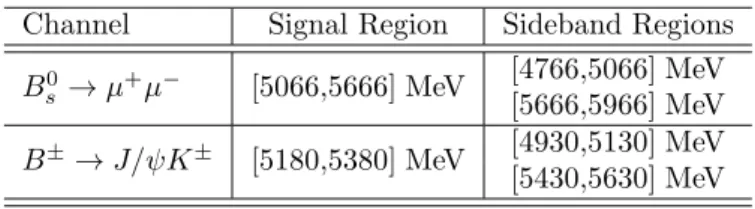
Channel Signal Region Sideband Regions
B0
s→µ+µ− [5066,5666] MeV
[4766,5066] MeV [5666,5966] MeV
B±→J/ψK± [5180,5380] MeV [4930,5130] MeV [5430,5630] MeV
Table 1: Definition of the signal and sideband regions used in this analysis.
The primary vertex position was obtained from a fit of charged tracks not used in the decay vertex and con-strained to the interaction region of the colliding beams. If multiple candidate primary vertices were present, the one closest inzto the decay vertex was chosen. After pre-selection, approximately 2·105 B0
s → µ+µ− and 1.4·105
B± →J/ψK± candidates were obtained in the signal re-gions.
Samples of Monte Carlo (MC) events were used for the extraction of acceptance and efficiency ratios. MC sam-ples were produced for the signal channel B0
s → µ+µ−,
the reference channelB± →J/ψK± (J/ψ →µ+µ−) and the control channel B0
s → J/ψφ (φ → K+K−). These
samples were generated with Pythia 6.4 [25] using the
2010 ATLAS [24, 26] tune. MC events were filtered be-fore detector simulation to ensure the presence of at least one decay of interest, with B decay products all satisfy-ing|η|<2.5 and pT >2.5 (0.5) GeV for muons (kaons).
An additional sample was generated with a fictitious value of the B0
s mass (6500 MeV) and the same parameters as
the standardB0
s →µ+µ−sample, allowing a check of the
full analysis on a signal-free region before unblinding. The ATLAS detector and its response were simulated using
Geant4[27]. Additionalppinteractions in the same and
3. Event selection
This Section describes the expected background com-position, the discriminating variables used as input to the multivariate classifier, the tuning of the simulation for the determination of the signal efficiency, the data samples used to estimate the background rejection and the opti-mization procedure. The signal efficiency was determined from MC samples, re-weighted to account for differences between data and MC simulation of theBmeson kinemat-ics. The rejection power was tested using a sub-sample of background events from the sidebands in the di-muon mass spectrum.
3.1. Background composition
Two categories of background were considered: a con-tinuum with a smooth dependence on the di-muon invari-ant mass, and sources of resoninvari-ant contributions from mis-reconstructed decays.
Comparisons of data and MC have shown that the com-binatorial background fromb¯b→µ+µ−X decays provides a reasonable description for the distributions of the dis-criminating variables for the events found in the sidebands. Theb¯b→µ+µ−X MC sample used is equivalent to about 12 pb−1of integrated luminosity. Such studies support the
procedure of modeling the continuum background through interpolation of the di-muon yield in the sidebands, but do not reach a sufficient statistical precision. Half of the data events in the sidebands (those with odd event num-bers) were used to optimize the selection procedure. The remaining events were used for the measurement of the background and for interpolation to the signal region.
Resonant background is due to B decay candidates containing either one or two hadrons erroneously identi-fied as muons. Mis-identification may be due to punch-through of a hadron to the MS or to decays in flight where the muon carries most of the hadron momentum. In either case the hadron fakes the muon signature for the purpose of this analysis. Single-fake events are due to, e.g. B0
s →K+µ−ν, the charged K meson being
mis-identified as a muon. Double-fake events are due to two-body hadronic B decays (B → hh), e.g. B0
s → K+π−,
where both hadrons are mis-identified as muons. MC studies have shown that double-fake events are the main source of resonant background after the selection crite-ria used in this analysis. The main contribution is from B0
s→K+K−, followed byB0→π+π− andB0→K±π∓
[20, 28].
The simulation determined the probability for a hadron to be misidentified as a muon to be equal to 2 (4)h for
π± (K±), with a relative uncertainty of 20%, validated against control samples in data [29]. The value for charged K mesons was averaged over K+ andK− and was found consistent with the preliminary results of data-driven stud-ies based on the decay D∗→D0π→Kππ.
The expected event yield for B → hh was obtained from an estimation of the integrated luminosity,
accep-tance and efficiency. This constitutes a nearly irreducible background in this analysis, due to its resemblance to the actual signal.
Variable Description
|α2D| Absolute value of the angle in the transverse
pointing angle plane between ∆~xand~pB
∆R Anglep
(∆φ)2+ (∆η)2 between ∆~xand~pB Lxy Scalar product in the transverse plane of
(∆~x·~pB)/|~pB
T|
ctsignificance Proper decay lengthct=Lxy×mB/p
B
T
divided by its uncertainty
χ2
xy,χ2z Vertex separation significance ∆~x
T· σ2
∆~x
−1 ·∆~x
in (x, y) andz, respectively
Ratio of|~pB
T|to the sum of|~p
B
T|and
I0.7 the transverse momenta of all tracks with
isolation pT>0.5 GeV within a cone ∆R <0.7 from
theBdirection, excludingBdecay products
|dmax
0 |,|dmin0 |
Absolute values of the maximum and minimum impact parameter in the transverse plane of theBdecay products relative to the primary vertex
|Dmin
xy |,|Dzmin|
Absolute values of the minimum distance of closest approach in thexyplane (or alongz) of tracks in the event to theBvertex
pB
T Btransverse momentum
pmax
L ,p
min L
Maximum and minimum momentum of the two muon candidates along theBdirection
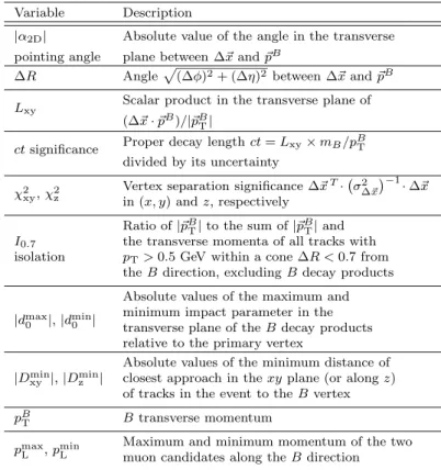
Table 2: List of the discriminating variables used in this analysis to separate B0
s → µ+µ− signal from backgrounds. These
vari-ables are based on properties of the decay products, of the recon-structed primary (~xPV) and secondary (~xSV) vertices (separated by
∆~x=~xSV−x~PV), theBmeson momentump~B and the properties
of additional tracks from the underlying event. Variables are listed in order of relevance as ranked by the multivariate classifier used in the final signal/background separation as discussed in Section 3.4.2.
3.2. Discriminating variables
Table 2 describes the discriminating variables used in the multivariate classifier. TheB0
s→µ+µ− signal is
char-acterized by the separation between the production (pri-mary) and decay (secondary) vertices, as well as the two-body decay topology. These variables exploit such fea-tures to discriminate against potential backgrounds: pairs of prompt charged tracks (e.g. Lxy, ct significance, χ2xy),
as well as pairs of displaced muons originating fromb¯b→
µ+µ−X processes (e.g. dmax
0 , dmin0 ), secondary vertices
with additional particles in the final state (e.g. α2D, ∆R,
Dxymin, Dzmin) and non-b¯b processes (e.g. I0.7, pBT, pmaxL ,
pmin L ).
Figure 1 shows how the discriminating variables are distributed for signal and background. Among the dis-criminating variables, isolation (I0.7) is expected to have
| 2D
α
|
0 0.5 1 1.5 2 2.5 3
Normalized Number of Events
10 2 10 3 10 4 10 5 10 | 2D α |
0 0.5 1 1.5 2 2.5 3
Normalized Number of Events
10 2 10 3 10 4 10 5 10 ATLAS
= 7 TeV s
-1 Ldt = 2.4 fb ∫
R
∆
0 1 2 3 4 5 6
Normalized Number of Events
1 10 2 10 3 10 4 10 5 10 R ∆
0 1 2 3 4 5 6
Normalized Number of Events
1 10 2 10 3 10 4 10 5 10 ATLAS = 7 TeV s
-1 Ldt = 2.4 fb ∫
[mm] xy L
0 1 2 3 4 5 6 7
Normalized Number of Events
1 10 2 10 3 10 4 10 [mm] xy L
0 1 2 3 4 5 6 7
Normalized Number of Events
1 10 2 10 3 10 4 10 ATLAS = 7 TeV s
-1 Ldt = 2.4 fb ∫
ct significance
-10 0 10 20 30 40 50 60 70
Normalized Number of Events
1 10 2 10 3 10 4 10 ct significance
-10 0 10 20 30 40 50 60 70
Normalized Number of Events
1 10 2 10 3 10 4 10 ATLAS = 7 TeV s
-1 Ldt = 2.4 fb ∫ ) z 2 χ Log(
-10 -5 0 5 10
Normalized Number of Events
0 2 4 6 8 10 3 10 × ) z 2 χ Log(
-10 -5 0 5 10
Normalized Number of Events
0 2 4 6 8 10 3 10 × ATLAS = 7 TeV s
-1 Ldt = 2.4 fb ∫ ) xy 2 χ Log(
-6 -4 -2 0 2 4 6 8 10 12
Normalized Number of Events
0 2 4 6 8 10 3 10 × ) xy 2 χ Log(
-6 -4 -2 0 2 4 6 8 10 12
Normalized Number of Events
0 2 4 6 8 10 3 10 × ATLAS = 7 TeV s
-1 Ldt = 2.4 fb ∫
) 0.7 Isolation (I
0 0.2 0.4 0.6 0.8 1
Normalized Number of Events
1 10 2 10 3 10 4 10 5 10 ) 0.7 Isolation (I
0 0.2 0.4 0.6 0.8 1
Normalized Number of Events
1 10 2 10 3 10 4 10 5 10 ATLAS = 7 TeV s
-1 Ldt = 2.4 fb ∫
|[mm] 0 max |d
0 0.5 1 1.5 2
Normalized Number of Events
1 10 2 10 3 10 4 10 |[mm] 0 max |d
0 0.5 1 1.5 2
Normalized Number of Events
1 10 2 10 3 10 4 10 ATLAS = 7 TeV s
-1 Ldt = 2.4 fb ∫
|[mm] 0 min |d
0 0.5 1 1.5 2
Normalized Number of Events
1 10 2 10 3 10 4 10 5 10 |[mm] 0 min |d
0 0.5 1 1.5 2
Normalized Number of Events
1 10 2 10 3 10 4 10 5 10 ATLAS = 7 TeV s
-1 Ldt = 2.4 fb ∫
|[mm] xy min |D
0 0.1 0.2 0.3 0.4 0.5
Normalized Number of Events
1 10 2 10 3 10 4 10 5 10 |[mm] xy min |D
0 0.1 0.2 0.3 0.4 0.5
Normalized Number of Events
1 10 2 10 3 10 4 10 5 10 ATLAS = 7 TeV s
-1 Ldt = 2.4 fb ∫
|[mm] z min |D
0 50 100 150 200 250 300 350
Normalized Number of Events
1 10 2 10 3 10 4 10 5 10 |[mm] z min |D
0 50 100 150 200 250 300 350
Normalized Number of Events
1 10 2 10 3 10 4 10 5 10 ATLAS = 7 TeV s
-1 Ldt = 2.4 fb ∫
[GeV] T B p
10 20 30 40 50 60
Normalized Number of Events
10 2 10 3 10 4 10 [GeV] T B p
10 20 30 40 50 60
Normalized Number of Events
10 2 10 3 10 4 10 ATLAS = 7 TeV s
-1 Ldt = 2.4 fb ∫
[GeV] max L P
5 10 15 20 25 30 35
Normalized Number of Events
10 2 10 3 10 4 10 [GeV] max L P
5 10 15 20 25 30 35
Normalized Number of Events
10 2 10 3 10 4 10 ATLAS = 7 TeV s
-1 Ldt = 2.4 fb ∫
[GeV] min L P
5 10 15 20 25 30 35
Normalized Number of Events
1 10 2 10 3 10 4 10 [GeV] min L P
5 10 15 20 25 30 35
Normalized Number of Events
1 10 2 10 3 10 4 10 ATLAS = 7 TeV s
-1 Ldt = 2.4 fb ∫
Figure 1: Signal (filled histogram) and sideband (empty histogram) distributions for the selection variables described in Table 2. The
B0
s →µ+µ− signal (normalized to the background histogram) is from simulation and the background is from data in the invariant-mass
include tracks originating from the primary vertex associ-ated with theBdecay. This specification makes the
selec-Number of primary vertices
0 2 4 6 8 10 12
Is o la ti o n c u t e ff ic ie n c y 0 0.1 0.2 0.3 0.4 0.5 0.6 0.7 0.8 0.9 1
MC isolation with PV association
MC isolation without PV association Data isolation with PV association Data isolation without PV association
ATLAS
= 7 TeV s
-1 Ldt = 2.4 fb
∫
Figure 2: Efficiency of the cutI0.7>0.83 as a function of the primary
vertex multiplicity for B±
→J/ψK±
candidate events from data (filled symbols) and MC simulation (empty symbols). The triangles show the efficiency when including all the tracks in the event, while circles show the same efficiency with the isolation definition used in this analysis.
tion independent of pile-up, as shown in Figure 2, where the efficiency of the selection for B± →J/ψK± is shown for events with different numbers of reconstructed primary vertices, both in sideband-subtracted data and MC.
The variable I0.7 might also be subject to differences
betweenB0
sandB±in the distributions of the surrounding
hadrons, e.g. with harderpT spectra for kaons produced in
association with theB0
s in the b-quark fragmentation. As
predicted by MC, significant differences were observed be-tweenB± →J/ψK±and the control channelB0
s→J/ψφ
in the I0.7 distribution from data. Within statistical
un-certainties, the I0.7 distribution from the MC simulation
of the control channel B0
s →J/ψφwas verified to be
con-sistent with the corresponding sideband-subtracted signal in data.
3.3. MC re-weighting and comparison to data
Monte Carlo samples were produced for the signal, ref-erence and control channels, with specific requirements on the B meson decay products as described above in Sec-tion 2. In order to ensure that the data are reproduced as closely as possible, the simulation was tuned by an it-erative weighting procedure: a generator-level (GL) re-weighting based on simulation, followed by a data driven (DD) re-weighting.
For the GL re-weighting, additional MC samples were generated without selection on the final states and over a wider range in theb-quark kinematics:
ηb
<4 andpbT>
2.5 GeV. These samples allowed a binned pB
T, ηB
map of
the efficiencies of the generator-level selections to be de-rived for both the signal and the reference MC. The inverse of such efficiencies was then used to weight events individ-ually, thus correcting the GL biases. These corrections were applied independently to the simulated reference and signal channel samples to correct for the biases in the rela-tiveB0
s/B± acceptance induced by the generator-level
se-lection. Possible residual biases were found to be negligible within the fiducial region
ηB
<2.5 and pBT >8.0 GeV.
Residual pB
T, ηB
differences between data and MC were observed after GL reweighting. These were addressed with the DD re-weighting procedure, based on the compar-ison of MC events to the large sample of B± →J/ψK± decays in collision data. In order not to correlate the re-weighting procedure with the yield measurement, only candidates with odd event numbers in the ATLAS dataset were used in this procedure, while the remaining sample was used for the yield measurement.
DD weights were determined by an iterative method, comparing re-weighted MC events with sideband-subtracted B±→J/ψK±events in data. The procedure was applied separately to theB meson variablespB
T andηB due to the
limited number of reconstructedB± →J/ψK± events in data, deriving the weights:
Wij(pBT, ηB) =wi(pBT)×wj(ηB) (3)
where W represents the final DD weights, the indices i andjrefer to bins inpB
TandηB, andwk =Nkdata/NkMCis
the data-to-MC ratio of the normalized number of entries for each variable. The convergence and the consistency of the procedure, together with the factorization assumption of Eq. 3, were tested with additional MC samples, where intentionally distorted (pB
T, ηB) spectra were found to
con-verge to the expected distributions. Effects related to the finite resolution in the measured variables were estimated to be smaller than 1hof the bin content and are therefore
negligible when compared to statistical uncertainties. Generator-level biases were addressed by applying the GL re-weighting before the DD re-weighting, and by verify-ing that this correction yields compatible (pB
T, ηB) spectra
forB0
s→µ+µ−andB± →J/ψK± MC samples. Finally,
the full re-weighting procedure was applied toB0
s →J/ψφ
decays, verifying within statistical uncertainty the consis-tency of the weights with those fromB±→J/ψK±.
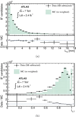
Distributions from B± → J/ψK± in MC simulation and data were compared, after side-band background sub-traction, for all discriminating variables listed in Table 2 and for variables used in the preselection. Agreement be-tween MC and data was found for most of the variables. Figure 3 shows comparisons for Lxy and I0.7.
0 2 4 6 8 10 12 14 16 18
candidates
±
B
0 1 2 3 4 5 6 7
3 10
×
Data (SB subtracted)
MC (re-weighted) ATLAS
= 7 TeV s
-1 Ldt = 2.4 fb
∫
[mm]
xy
L
0 2 4 6 8 10 12 14 16 18
Data / MC 0.5
1
(a)
0 0.2 0.4 0.6 0.8 1
candidates
±
B
0 0.5 1 1.5 2 2.5 3 3.5 4 4.5
3 10
×
Data (SB subtracted)
MC (re-weighted)
ATLAS
= 7 TeV s
-1 Ldt = 2.4 fb
∫
0.7
I
0 0.2 0.4 0.6 0.8 1
Data / MC 1
2
(b)
Figure 3: Examples of sideband-subtracted data-reweighted MC comparisons usingB±
→J/ψK±
decays for two of the most pow-erful separation variables: (a)Lxy and (b)I0.7. Uncertainties are
statistical only. The lower graph in each case shows the data/MC ratio.
3.4. Selection optimization
The optimization of the event selection was performed by maximizing the estimator:
P = a ǫsig
2 +
p
Nbkg
, (4)
where ǫsig =Aµ+µ−ǫµ+µ− and Nbkg are the signal
accep-tance times efficiency relative to the simulated phase space of the samples in section 3.3 (corresponding to the signal efficiency defined for|ηB|<2.5 andpB
T >8.0 GeV) and the
background yield for a given set of cuts. The extraction of Nbkg is performed by sideband interpolation as described
in section 5. The coefficientawas determined by the con-fidence level (CL) sought in the analysis, with a=2 for a 95% CL limit. This quantity is specifically designed to op-timize the performance of a frequentist limit determination in a counting analysis [30].
First, a simplified optimization procedure was performed on a small set of variables that includes: |α2D|, I0.7, ct,
and width±∆mof the search window centred around the B0
s mass (rounded to 5366 MeV). A four-dimensional scan
was performed on the four variables, using odd-numbered
events in the sidebands. The optimal selection cuts are shown in Table 3, where the signal efficiencyAµ+µ−ǫµ+µ−,
the background estimated from sidebands interpolation and the value of P are also given. This selection serves as a benchmark for the optimization of the multivariate analysis described in Section 3.4.2.
|α2D| ct I0.7 ∆m ǫsig Nbkg P
<0.03 >0.3 mm >0.83 ±105 MeV 0.040 9±2 0.010
Table 3: Optimal selection variable cuts for the four-variables scan, and resulting analysis performance in terms of signal acceptance times efficiency (ǫsig), background yield in the signal region (Nbkg)
and the estimatorP.
3.4.1. Categories of invariant-mass resolution The ability to resolve a small B0
s →µ+µ− signal from
the continuum background depends on the width ∆mof the search region and is therefore affected by the reso-lution. The latter varies considerably over different sub-samples of muon pairs measured by ATLAS, due to the increase in multiple scattering and the decrease of the mag-netic field integral at large values of|η|. The non-resonant background invariant mass distribution was observed to be relatively independent ofη. As a consequence, different mass-resolution categories correspond to different signal-to-background conditions.
In the statistical analysis, regions of different mass res-olution and hence signal-to-background ratio were sepa-rated in order to optimize them independently. The sam-ple was separated into three categories, defined by the larger pseudorapidity value |η|max of the two muons in
each event. The three categories were defined by the inter-vals|η|max = 0–1, 1–1.5 and 1.5–2.5. The corresponding
average values of the mass resolution are approximately 60, 80 and 110 MeV, respectively. The relative population of each interval, in B0
s → µ+µ− signal MC, amounts to
51%, 24% and 25%.
The same classification, based on|η|max, was used for
the reference channelB± →J/ψK±, and separate values of the acceptance-times-efficiency ratio were obtained for each category, as discussed in Section 4.1.
3.4.2. Multivariate selection
The selection with optimal cuts was used to validate the multivariate analysis tool used for the final results. The TMVA package [31] implementation of Boosted De-cision Trees (BDT) was found to have the best perfor-mance and was selected for this analysis. As a first step, it was verified that for fixed values of ∆m, the optimal BDT corresponds to selections in the variablesα2D,ct and
I0.7 directly comparable to those obtained with the cuts
the P estimator improved from P = 0.010 found in the simplified optimization toP = 0.016.
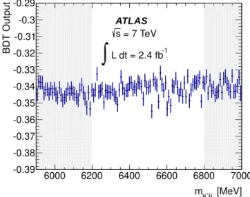
In order to avoid biases in the background interpola-tion, the BDT selection should be insensitive to the mass of the muon pair. The BDT inputs have no correlation with the invariant mass. Residual correlations in the BDT output were studied through the search for a fictitious de-cay X → µ+µ− with m
X = 6500 MeV. A Monte Carlo
sample was used to provide reference signal events, while data in the mass intervals 5900 to 6200 MeV and 6800 to 7000 MeV were used as background. The BDT training and selection optimization were consistently performed on odd-numbered events. Figure 4 shows the BDT output as a function of the di-muon mass, over the sideband re-gions and the fictitious signal region (6200 to 6800 MeV), which was not used in the optimization. No significant mass dependence was observed.
[MeV]
-µ
+
µ
m
6000 6200 6400 6600 6800 7000
B
D
T
O
u
tp
u
t
-0.39 -0.38 -0.37 -0.36 -0.35 -0.34 -0.33 -0.32 -0.31 -0.3 -0.29
ATLAS
= 7 TeV s
-1
L dt = 2.4 fb
∫
Figure 4: Mean and RMS (error bars) of the BDT output in bins of di-muon invariant mass, for background events in the region 5900 to 7000 MeV, with the 6200 to 6800 MeV region not used in the training of the classifier. The BDT used is the one trained for the search of the fictitious 6500 MeV signal.
The optimization of the multivariate analysis was per-formed in the six-dimensional space of ∆m and the BDT output cuts for each of the mass-resolution categories. The independence of the BDT output onmµ+µ− and the
com-plementarity of the samples allow the factorization of the individual cut efficiencies. Each efficiency curve was in-terpolated with analytical models, allowing the numerical maximization ofP and yielding the optimal cuts reported in Table 4.
4. Single Event Sensitivity ingredients
4.1. Relative acceptance and efficiency
The ratio of the acceptance times efficiency products for the charged and neutral decays
RAǫ= (AJ/ψKǫJ/ψK)/(Aµ+µ−ǫµ+µ−)
|η|max Range 0–1.0 1.0–1.5 1.5–2.5
invariant mass window [MeV] ±116 ±133 ±171 BDT output threshold 0.234 0.245 0.270
Table 4: BDT output and ∆mcuts for each mass-resolution category, optimized according to the method described in the text.
is required for the determination of the SES (Eq. 1). The same BDT, trained on the B0
s signal MC sample and
di-muon data sidebands, was used to select both decay modes. The uncertainty on RAǫ is affected by differences
be-tween data and MC in the distributions of the discriminat-ing variables. Such differences are reduced by the data-driven corrections applied to the MC B-meson kinemat-ics. Furthermore, only deviations that act incoherently between the signal and the reference channel contribute to the uncertainty on RAǫ. These effects were studied by
observing the change in the relative efficiency of the BDT selection when the simulated events were re-weighted by the data-to-MC ratio of the distributions of the most sen-sitive variables in B± → J/ψK± events. The procedure was performed with the cut on the BDT output fixed at the optimal value for each of the three event categories. Conservatively, the corresponding variations inRAǫ were
combined linearly and taken as systematic uncertainties. Due to large correlations between Lxy, χ2xy and ct
-significance, correcting for the differences in Lxy between
data and simulation was found to also effectively remove differences in the other two variables. Therefore onlyLxy
was considered, since it induced the largest deviation in RAǫ. Differences in theη andpTdistributions of the final
state particles, the hit multiplicity in the Pixel detector, and the multiplicity of reconstructed primary vertices were included in the systematic uncertainty evaluation.
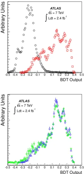
Figure 5 shows the distribution of the BDT output for MC samples of B0
s → µ+µ− and B± → J/ψK± decays,
with a signal–background comparison forB0
s→µ+µ−and
a sideband-subtracted data–MC comparison for B± → J/ψK±. As shown in Table 4, the selection required the BDT output to exceed 0.23–0.27, depending on the mass-resolution category. The systematic uncertainties induce a fractional change in the number of events passing the BDT cut varying between 10% and 20% depending on the category. This change is highly correlated between the two channels: the corresponding variation on the efficiency ra-tio is 0.6%, which was taken as a systematic uncertainty and is smaller than the ±2.3% error due to the finite MC statistics.
The value ofRAǫand its systematic uncertainties (shown
0.011 (syst) for MC.
Additional smaller contributions to the uncertainty on RAǫ are due to the data-MC discrepancy in vertex
recon-struction efficiency (±2%) [24], the uncertainty on the ab-solute K± reconstruction efficiency as derived from simu-lation of the B±→J/ψK± reference channel (±5%) and asymmetry differences in detector response toK+andK− mesons (±1%).
BDT Output
-0.5 -0.4 -0.3 -0.2 -0.1 0 0.1 0.2 0.3 0.4 0.5
Arbitrary Units
ATLAS
= 7 TeV s
-1 Ldt = 2.4 fb
∫
BDT Output
-0.5 -0.4 -0.3 -0.2 -0.1 0 0.1 0.2 0.3 0.4 0.5
Arbitrary Units
ATLAS
= 7 TeV s
-1 Ldt = 2.4 fb
∫
Figure 5: Distributions of the response of the BDT classifier. Top:
B0
s → µ+µ− MC sample (squares) and data sidebands (circles);
bottom: B±
→J/ψK±
events from tuned MC samples (triangles) and sideband-subtracted data (stars).
4.2. B±→J/ψK± event yield
The reference channel yield NJ/ψK± was determined
from a binned likelihood fit to the invariant mass distribu-tion of theµ+µ−K± system, performed in the mass range 4930-5630 MeV. To avoid any bias induced by the DD re-weighting of the MC samples discussed in Section 3.3, only even-numbered events were used in the extraction of the B± → J/ψK± event yield. The B± signal was modelled with two Gaussian distributions of equal mean
|η|max RiAǫ ∆ % ∆ %
Range Stat. Syst.
0–1.0 0.274 3.1 3.1 1.0–1.5 0.202 4.8 5.5 1.5–2.5 0.143 5.3 5.9
Table 5: Values of the acceptance-times-efficiency ratio RAǫ
be-tween reference and search channel, shown separately for the differ-ent categories in mass-resolution.
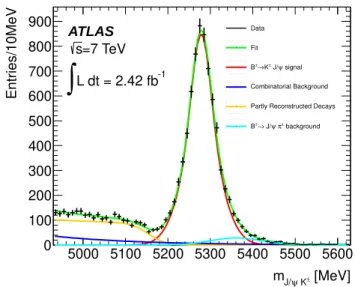
value. The background was modelled with the sum of: (a) an exponential function for the continuum combinato-rial background; (b) an exponential function multiplied by a complementary error function describing the low-mass (m <5200 MeV) contribution for partially reconstructed decays (such as B → J/ψK∗, B → J/ψK(1270) and B → χcK); and (c) a Gaussian function for the
back-ground fromB± →J/ψπ±. Figure 6 shows the invariant mass distribution and the result of the fit for the selected data sample.
All parameters describing the signal and background were determined from the fit, with the exception of the mass and the width of the last component (c), which were obtained from simulation. The fit was performed for each of the three categories of mass resolution.
Systematic uncertainties affecting the extracted refer-ence yield were estimated by varying the fit model: use of different bin sizes (10 or 25 MeV and unbinned), differ-ent models for signal and continuum background, inclusion of event-wise di-muon mass resolution. The resultingB± yields are given with their statistical and systematic un-certainties in Table 6.
|η|max Range 0–1.0 1.0–1.5 1.5–2.5
B±→J/ψK±→µ+µ−K± 4300 1410 1130 statistical uncertainty ±1.6% ±2.8% ±3.0% systematic uncertainty ±2.9% ±7.4% ±14.1%
Table 6: Event yield for even-numbered candidates in the reference channel.
5. Inputs to the limit extraction
The evaluation of the SES requires as input the com-bined branching fraction for the reference channelB± → J/ψK±→ µ+µ−K±, which is (6.01±0.21)×10−5 [20].
The relative production rate of B0
s relative to B± fs/fu
is 0.267±0.021 [22], assuming fu = fd (following Ref.
[21]) and no kinematic dependence offs/fu. The ratio of
acceptance-times-efficiency is discussed in Section 4 and presented in Table 5. The branching fractions uncertain-ties, those onfu/fs, together with those mentioned in the
[MeV] ± K ψ J/ m
5000 5100 5200 5300 5400 5500 5600
Entries/10MeV 0 100 200 300 400 500 600 700 800 900 -1
L dt = 2.42 fb
∫
=7 TeV s ATLAS Data Fit signal ψ J/ ± K → ± B Combinatorial BackgroundPartly Reconstructed Decays
background ± π ψ J/ → ± B
Figure 6: J/ψK±
mass distribution for all theB±
candidates from even-numbered events passing all the selection cuts, merged for il-lustration purposes. Curves in the plot correspond to the various fit components: two Gaussians with a common mean for the main peak, a single Gaussian with higher mean for the B± →J/ψπ±
decay, a falling exponential for the continuum background and an exponential function multiplying a complementary error function for the partially reconstructed decays.
In each mass-resolution category theB0
s →µ+µ−
sig-nal yieldNµ+µ− was obtained from the number of events
observed in the search window, the number of background events in the sidebands, and the small amount of resonant background discussed in Section 3.1. The expected ratio of the background events in the sidebands to those in the search window is described by the parameterRbkgi , which depends on the width of the invariant-mass interval and on the fraction of events from the sidebands used for the interpolation. The former varies according to the mass-resolution category, and the latter is equal to 50%, corre-sponding to the even-numbered events in the data collec-tion. Uncertainties in the mass dependence of the contin-uum background produced a±4% systematic error in the value ofRbkgi , evaluated by studying the variation ofR
bkg
i
for different BDT output cuts and background interpola-tion models. The systematic variainterpola-tion accounts also for additional background components in the low mass side-bands (e.g. partially reconstructed B decays). This uncer-tainty was treated coherently in the three mass-resolution categories.
The values of the SES are given in Table 7 which also shows the values of the parametersRbkgi , the background counts in the sidebands2, the resonant background, and
finally the observed number of events in the search region,
2For comparison, the number of odd-numbered events observed
in the sidebands, which is expected to be biased due to the use of the same sample in selection optimization and BDT training, was found to be equal to one event in each of the three mass-resolution categories.
as found after unblinding. Figure 7 shows the invariant mass distribution of the selected candidates in data, for the three mass categories, together with the signal projections as obtained from MC assuming BR(B0
s →µ+µ−) = 3.5·
10−8 (i.e. approximately 10 times the SM expectation).
[MeV]
µ µ
m 4800 5000 5200 5400 5600 5800
Events/60 MeV 0 0.5 1 1.5 2 2.5 3 3.5 ATLAS
= 7 TeV s
-1
Ldt = 2.4 fb
∫
< 1 max | η | Data ) × MC (10 -µ + µ → s B [MeV] µ µ m 4800 5000 5200 5400 5600 5800Events/60 MeV 0 0.5 1 1.5 2 2.5 3 3.5 ATLAS
= 7 TeV s
-1
Ldt = 2.4 fb
∫
< 1.5 max | η | Data ) × MC (10 -µ + µ → s B [MeV] µ µ m 4800 5000 5200 5400 5600 5800Events/60 MeV 0 0.5 1 1.5 2 2.5 3 3.5 ATLAS
= 7 TeV s
-1
Ldt = 2.4 fb
∫
< 2.5 max | η | Data ) × MC (10 -µ + µ → s BFigure 7: Invariant mass distribution of candidates in data. For each mass-resolution category (top to bottom) each plot shows the invariant mass distribution for the selected candidates in data (dots), the signal (continuous line) as predicted by MC assuming BR(B0
s →
µ+µ−
) = 3.5·10−8, and two dashed vertical lines corresponding to
|η|max Range 0–1.0 1.0–1.5 1.5–2.5
SES= (ǫǫi)−1 [10−8] 0.71 1.6 1.4
ǫ= (fs/fu)/BR(B±→J/ψK±→µ+µ−K±) [103] 4.45±0.38
ǫi=NB
±
→J/ψK±
i /RiAǫ[104] 3.14±0.17 1.40±0.15 1.58±0.26
bkg. scaling factor Rbkgi 1.29 1.14 0.88
sideband count Nobsbkg,i(even numbered events) 5 0 2 expected resonant bkg. NB→hh
i 0.10 0.06 0.08
search region countNiobs 2 1 0
Table 7: Single event sensitivity and event counts in the three mass resolution categories. The second and third lines report how the SES= (ǫǫi)−1 was split between a coefficient common to all bins, and the per-bin component. The Table does not include the additional
common uncertainties corresponding the sources mentioned in the last paragraph of Section 4.1 (±5.5% inRi
Aǫ) and to the parameterization
of the mass dependence of the continuum background (±4% inRbkgi ).
6. Branching fraction limits
The upper limit on theB0
s→µ+µ− branching fraction
was obtained by means of an implementation [32] of the CLs method [33]. The extraction was based on the
likeli-hood:
L = Gauss(ǫobs|ǫ, σǫ)×Gauss(Rbkgobs|Rbkg, σRbkg)× Nbin
Y
i=1
Poisson(Niobs|ǫ ǫiBR +Nibkg+NiB→hh)×
Poisson(Nobsbkg,i|RbkgRbkgi Nibkg)×
Gauss(ǫobs,i|ǫi, σǫi).
For each mass-resolution category, the likelihood contains Poisson distributions for the event counts in the search and sideband regions and a Gaussian distribution for the rel-ative efficiencyǫi. Two additional Gaussians describe the
coherent systematic uncertainties inRbkgand in the SES.
The mean of the Poisson distribution in the search region is equal to the sum of the B0
s branching fraction (scaled
by the normalization and relative efficiency parameters), the continuum background and the resonant background. The mean of the Poisson distribution in the sidebands is equal to the background scaled by Rbkg. The parameters
σǫ(σǫi),σRbkg (σRbkg
i ) account for the correlated
(uncorre-lated) uncertainties in the SES and the background scaling factor. In this analysis the uncertainties onRbkgi are
neg-ligible, withRbkg= 1.00±0.04. All input parameters are
summarized in Table 7.
The expected limits were obtained by setting the counts in the search region equal to the interpolated background plus the small resonant background, before the unblinding of the signal region. A median expected limit of 2.3+1−0..05×
10−8 at 95% CL was obtained, where the range encloses
68% of the background-only pseudo-experiments.
For comparison the mass-resolution categories were merged and the selection optimization was performed on the merged sample. In this case eight events were found in the side-bands, resulting in a branching fraction limit of 2.9+1−0..38×
10−8 at 95% CL. This test confirms the expectation of a
more sensitive analysis when separate mass-resolution cat-egories are used.
The background counts found in odd-numbered events were used to assess the magnitude of the bias that would be caused by using the same sample for selection opti-mization and the estimation ofNbkg. The expected limit
obtained using the same sample for optimization and sig-nal extraction is 1.7×10⁻⁸, about 30% smaller than the
limit presented in this Letter, for which independent sam-ples were used for optimization and for signal extraction. The observed bias is consistent with simulation-based as-sessments of this effect.
Figure 8 shows the behaviour of the observed CLs for
different tested values of theB0
s →µ+µ− branching
frac-tion, computed with 300 000 toy MC simulations per point. The observed limit is<2.2 (1.9)×10−8at 95% (90%) CL.
Thep-values for the background-only hypothesis and for background plus SM prediction [1, 2] are 44% and 35%, respectively.
]
-8
)[10
-µ
+
µ →
s 0
BR(B
0 1 2 3 4 5
s
CL
-3
10
-2
10
-1
10 1
Observed CLs Expected CLs - Median
σ
1
±
Expected CLs
σ
2
±
Expected CLs
ATLAS
= 7 TeV s
-1
Ldt = 2.4 fb
∫
Figure 8: Observed CLs (circles) as a function of BR(Bs0→µ+µ−).
The 95% CL limit is indicated by the horizontal (red) line. The dark (green) and light (yellow) bands correspond to±1σ and ±2σ
Despite the difference between the total numbers of observed and interpolated background events (equal to 3 and 6.5, respectively), the interplay of the event counts observed in the three mass resolution categories produced an observed CLslimit close to the expected value.
7. Conclusions
A limit on the branching fraction BR(B0
s → µ+µ−)
is set using 2.4 fb−1 of integrated luminosity collected in
2011 by the ATLAS detector. The processB±→J/ψK±, with J/ψ→µ+µ−, is used as a reference channel for the normalization of integrated luminosity, acceptance and ef-ficiency. The final selection is based on a multivariate analysis performed on three categories of events deter-mined according to their mass resolution, yielding a limit of BR(B0
s →µ+µ−)<2.2 (1.9)×10−8at 95% (90%) CL.
8. Acknowledgements
We thank CERN for the very successful operation of the LHC, as well as the support staff from our institutions without whom ATLAS could not be operated efficiently.
We acknowledge the support of ANPCyT, Argentina; YerPhI, Armenia; ARC, Australia; BMWF, Austria; ANAS, Azerbaijan; SSTC, Belarus; CNPq and FAPESP, Brazil; NSERC, NRC and CFI, Canada; CERN; CONICYT, Chile; CAS, MOST and NSFC, China; COLCIENCIAS, Colom-bia; MSMT CR, MPO CR and VSC CR, Czech Repub-lic; DNRF, DNSRC and Lundbeck Foundation, Denmark; EPLANET and ERC, European Union; IN2P3-CNRS, CEA-DSM/IRFU, France; GNAS, Georgia; BMBF, DFG, HGF, MPG and AvH Foundation, Germany; GSRT, Greece; ISF, MINERVA, GIF, DIP and Benoziyo Center, Israel; INFN, Italy; MEXT and JSPS, Japan; CNRST, Morocco; FOM and NWO, Netherlands; RCN, Norway; MNiSW, Poland; GRICES and FCT, Portugal; MERYS (MECTS), Roma-nia; MES of Russia and ROSATOM, Russian Federation; JINR; MSTD, Serbia; MSSR, Slovakia; ARRS and MVZT, Slovenia; DST/NRF, South Africa; MICINN, Spain; SRC and Wallenberg Foundation, Sweden; SER, SNSF and Can-tons of Bern and Geneva, Switzerland; NSC, Taiwan; TAEK, Turkey; STFC, the Royal Society and Leverhulme Trust, United Kingdom; DOE and NSF, United States of Amer-ica.
The crucial computing support from all WLCG part-ners is acknowledged gratefully, in particular from CERN and the ATLAS Tier-1 facilities at TRIUMF (Canada), NDGF (Denmark, Norway, Sweden), CC-IN2P3 (France), KIT/GridKA (Germany), INFN-CNAF (Italy), NL-T1 (Nether-lands), PIC (Spain), ASGC (Taiwan), RAL (UK) and BNL (USA) and in the Tier-2 facilities worldwide.
References
[1] A. J. Buras, G. Isidori and P. Paradisi, EDMs versus CPV in
Bs,dmixing in two Higgs doublet models with MFV, Phys.Lett.
B694 (2011) 402–409.
[2] A. J. Buras, Minimal flavour violation and beyond: Towards a flavour code for short distance dynamics, Acta Phys.Polon. B41 (2010) 2487–2561.
[3] UTfit Collaboration, M. Bona et al., Standard Model up-dates and new physics analysis with the Unitarity Triangle fit. PoS(EPS-HEP2011)-2011-185.
[4] CKMfitter Collaboration, J. Charles et al., CP violation and the CKM matrix: Assessing the impact of the asymmetric B factories, Eur. Phys. J. C41 (2005) 1–131.
[5] L. J. Hall, R. Rattazzi and U. Sarid, The Top quark mass in su-persymmetric SO(10) unification, Phys.Rev. D50 (1994) 7048– 7065.
[6] C. Hamzaoui, M. Pospelov and M. Toharia, Higgs medi-ated FCNC in supersymmetric models with large tan Beta, Phys.Rev. D59 (1999) 095005.
[7] K. S. Babu and C. F. Kolda, Higgs mediated B0 →µ+µ−
in minimal supersymmetry, Phys.Rev.Lett. 84 (2000) 228–231. [8] S. Choudhury, A. S. Cornell, N. Gaur and G. C. Joshi,
Sig-natures of new physics in dileptonic B-decays, Int.J.Mod.Phys. A21 (2006) 2617–2634.
[9] J. Parry, Lepton flavor violating Higgs boson decays,τ →µγ
andBs→µ+µ−in the constrained MSSM+NR with large tan
beta, Nucl.Phys. B760 (2007) 38–63.
[10] J. R. Ellis, K. A. Olive, Y. Santoso and V. C. Spanos, OnBs→ µ+µ−
and cold dark matter scattering in the MSSM with non-universal Higgs masses, JHEP 0605 (2006) 063.
[11] J. R. Ellis, J. S. Lee and A. Pilaftsis, B-Meson Observables in the Maximally CP-Violating MSSM with Minimal Flavour Violation, Phys.Rev. D76 (2007) 115011.
[12] S. Davidson and S. Descotes-Genon, Minimal Flavour Violation for Leptoquarks, JHEP 1011 (2010) 073.
[13] D0 Collaboration, V. Abazov et al., Search for the rare decay
B0
s→µ+µ
−
, Phys.Lett. B693 (2010) 539–544.
[14] CDF Collaboration, T. Aaltonen et al., Search forBs→µ+µ−
and Bd → µ+µ− Decays with CDF II, Phys.Rev.Lett. 107
(2011) 239903.
[15] CMS Collaboration, Search forB0
sandB0to dimuon decays in ppcollisions at 7 TeV, Phys.Rev.Lett. 107 (2011) 191802. [16] CMS Collaboration, Search forB0
s →µµandB0→µµdecays,
arXiv:1203.3976.
[17] LHCb Collaboration, R. Aaij et al., Search for the rare decays
B0→µ+µ−
andB0
s→µ+µ−, Phys. Lett. B708 (2012) 55.
[18] LHCb Collaboration, R. Aaij et al., Strong constraints on the rare decaysB0
s→µ+µ−andB0→µ+µ−,arXiv:1203.4493.
[19] ATLAS Collaboration, The ATLAS Experiment at the CERN Large Hadron Collider, JINST 3 (2008) S08003.
[20] Particle Data Group, K. Nakamura et al., Review of Particle Physics, J. Phys. G 37 (7A) (2010) 075021.
[21] Heavy Flavor Averaging Group, D. Asner et al., Averages of
b-hadron,c-hadron, andτ-lepton Properties,arXiv:1010.1589. [22] LHCb Collaboration, R. Aaij et al., Measurement ofb hadron production fractions in 7 TeV pp collisions, Phys. Rev. D85 (2012) 032008.
[23] ATLAS Collaboration, Performance of the ATLAS Trigger Sys-tem in 2010, Eur. Phys. J. C72 (2012) 1849.
[24] ATLAS Collaboration, Charged-particle multiplicities in pp in-teractions measured with the ATLAS detector at the LHC, New J. Phys. 13 (2011) 053033.
[25] T. Sjostrand, S. Mrenna and P. Z. Skands, PYTHIA 6.4 Physics and Manual, JHEP 0605 (2006) 026.
[26] A. Buckley, ATLAS Monte Carlo generator tunes to LHC data, Nuclear Science Symposium Conference Record (NSS/MIC), 2010 IEEE (2010) 167–173.
[27] GEANT4 Collaboration, S. Agostinelli et al., GEANT4: A sim-ulation toolkit, Nucl. Instr. Meth. A506 (2003) 250303. [28] CDF Collaboration, T. Aaltonen et al., Evidence for the
charm-less annihilation decay modeB0
s→π+π−,arXiv:1111.0485.
[29] ATLAS Collaboration, Muon Reconstruction Performance, ATLAS-CONF-2010-064.
[31] A. Hoecker, P. Speckmayer, J. Stelzer, J. Therhaag, E. von Toerne, and H. Voss, TMVA 4: Toolkit for Multivariate Data Analysis, PoS ACAT 040.
[32] T. Junk, Confidence Level Computation for Combining Searches with Small Statistics, Nucl. Instrum. Meth. A434 (1999) 435– 443.
[33] A. L. Read, Presentation of search results: TheCLstechnique,
The ATLAS Collaboration
G. Aad48, B. Abbott111, J. Abdallah11, S. Abdel Khalek115, A.A. Abdelalim49, O. Abdinov10, B. Abi112, M. Abolins88,
O.S. AbouZeid158, H. Abramowicz153, H. Abreu136, E. Acerbi89a,89b, B.S. Acharya164a,164b, L. Adamczyk37,
D.L. Adams24, T.N. Addy56, J. Adelman176, S. Adomeit98, P. Adragna75, T. Adye129, S. Aefsky22,
J.A. Aguilar-Saavedra124b,a, M. Aharrouche81, S.P. Ahlen21, F. Ahles48, A. Ahmad148, M. Ahsan40, G. Aielli133a,133b,
T. Akdogan18a, T.P.A. ˚Akesson79, G. Akimoto155, A.V. Akimov94, A. Akiyama66, M.S. Alam1, M.A. Alam76,
J. Albert169, S. Albrand55, M. Aleksa29, I.N. Aleksandrov64, F. Alessandria89a, C. Alexa25a, G. Alexander153,
G. Alexandre49, T. Alexopoulos9, M. Alhroob164a,164c, M. Aliev15, G. Alimonti89a, J. Alison120, B.M.M. Allbrooke17,
P.P. Allport73, S.E. Allwood-Spiers53, J. Almond82, A. Aloisio102a,102b, R. Alon172, A. Alonso79, B. Alvarez Gonzalez88,
M.G. Alviggi102a,102b, K. Amako65, C. Amelung22, V.V. Ammosov128, A. Amorim124a,b, N. Amram153,
C. Anastopoulos29, L.S. Ancu16, N. Andari115, T. Andeen34, C.F. Anders20, G. Anders58a, K.J. Anderson30,
A. Andreazza89a,89b, V. Andrei58a, X.S. Anduaga70, A. Angerami34, F. Anghinolfi29, A. Anisenkov107, N. Anjos124a,
A. Annovi47, A. Antonaki8, M. Antonelli47, A. Antonov96, J. Antos144b, F. Anulli132a, S. Aoun83, L. Aperio Bella4,
R. Apolle118,c, G. Arabidze88, I. Aracena143, Y. Arai65, A.T.H. Arce44, S. Arfaoui148, J-F. Arguin14, E. Arik18a,∗, M. Arik18a, A.J. Armbruster87, O. Arnaez81, V. Arnal80, C. Arnault115, A. Artamonov95, G. Artoni132a,132b,
D. Arutinov20, S. Asai155, R. Asfandiyarov173, S. Ask27, B. ˚Asman146a,146b, L. Asquith5, K. Assamagan24,
A. Astbury169, B. Aubert4, E. Auge115, K. Augsten127, M. Aurousseau145a, G. Avolio163, R. Avramidou9, D. Axen168,
G. Azuelos93,d, Y. Azuma155, M.A. Baak29, G. Baccaglioni89a, C. Bacci134a,134b, A.M. Bach14, H. Bachacou136,
K. Bachas29, M. Backes49, M. Backhaus20, E. Badescu25a, P. Bagnaia132a,132b, S. Bahinipati2, Y. Bai32a,
D.C. Bailey158, T. Bain158, J.T. Baines129, O.K. Baker176, M.D. Baker24, S. Baker77, E. Banas38, P. Banerjee93,
Sw. Banerjee173, D. Banfi29, A. Bangert150, V. Bansal169, H.S. Bansil17, L. Barak172, S.P. Baranov94,
A. Barbaro Galtieri14, T. Barber48, E.L. Barberio86, D. Barberis50a,50b, M. Barbero20, D.Y. Bardin64, T. Barillari99,
M. Barisonzi175, T. Barklow143, N. Barlow27, B.M. Barnett129, R.M. Barnett14, A. Baroncelli134a, G. Barone49,
A.J. Barr118, F. Barreiro80, J. Barreiro Guimar˜aes da Costa57, P. Barrillon115, R. Bartoldus143, A.E. Barton71,
V. Bartsch149, R.L. Bates53, L. Batkova144a, J.R. Batley27, A. Battaglia16, M. Battistin29, F. Bauer136, H.S. Bawa143,e,
S. Beale98, T. Beau78, P.H. Beauchemin161, R. Beccherle50a, P. Bechtle20, H.P. Beck16, S. Becker98, M. Beckingham138,
K.H. Becks175, A.J. Beddall18c, A. Beddall18c, S. Bedikian176, V.A. Bednyakov64, C.P. Bee83, M. Begel24,
S. Behar Harpaz152, P.K. Behera62, M. Beimforde99, C. Belanger-Champagne85, P.J. Bell49, W.H. Bell49, G. Bella153,
L. Bellagamba19a, F. Bellina29, M. Bellomo29, A. Belloni57, O. Beloborodova107,f, K. Belotskiy96, O. Beltramello29,
O. Benary153, D. Benchekroun135a, K. Bendtz146a,146b, N. Benekos165, Y. Benhammou153, E. Benhar Noccioli49,
J.A. Benitez Garcia159b, D.P. Benjamin44, M. Benoit115, J.R. Bensinger22, K. Benslama130, S. Bentvelsen105,
D. Berge29, E. Bergeaas Kuutmann41, N. Berger4, F. Berghaus169, E. Berglund105, J. Beringer14, P. Bernat77,
R. Bernhard48, C. Bernius24, T. Berry76, C. Bertella83, A. Bertin19a,19b, F. Bertolucci122a,122b, M.I. Besana89a,89b, N. Besson136, S. Bethke99, W. Bhimji45, R.M. Bianchi29, M. Bianco72a,72b, O. Biebel98, S.P. Bieniek77, K. Bierwagen54,
J. Biesiada14, M. Biglietti134a, H. Bilokon47, M. Bindi19a,19b, S. Binet115, A. Bingul18c, C. Bini132a,132b, C. Biscarat178,
U. Bitenc48, K.M. Black21, R.E. Blair5, J.-B. Blanchard136, G. Blanchot29, T. Blazek144a, C. Blocker22, J. Blocki38,
A. Blondel49, W. Blum81, U. Blumenschein54, G.J. Bobbink105, V.B. Bobrovnikov107, S.S. Bocchetta79, A. Bocci44,
C.R. Boddy118, M. Boehler41, J. Boek175, N. Boelaert35, J.A. Bogaerts29, A. Bogdanchikov107, A. Bogouch90,∗, C. Bohm146a, J. Bohm125, V. Boisvert76, T. Bold37, V. Boldea25a, N.M. Bolnet136, M. Bomben78, M. Bona75,
M. Bondioli163, M. Boonekamp136, C.N. Booth139, S. Bordoni78, C. Borer16, A. Borisov128, G. Borissov71,
I. Borjanovic12a, M. Borri82, S. Borroni87, V. Bortolotto134a,134b, K. Bos105, D. Boscherini19a, M. Bosman11,
H. Boterenbrood105, D. Botterill129, J. Bouchami93, J. Boudreau123, E.V. Bouhova-Thacker71, D. Boumediene33,
C. Bourdarios115, N. Bousson83, A. Boveia30, J. Boyd29, I.R. Boyko64, N.I. Bozhko128, I. Bozovic-Jelisavcic12b,
J. Bracinik17, P. Branchini134a, A. Brandt7, G. Brandt118, O. Brandt54, U. Bratzler156, B. Brau84, J.E. Brau114,
H.M. Braun175, B. Brelier158, J. Bremer29, K. Brendlinger120, R. Brenner166, S. Bressler172, D. Britton53,
F.M. Brochu27, I. Brock20, R. Brock88, E. Brodet153, F. Broggi89a, C. Bromberg88, J. Bronner99, G. Brooijmans34,
W.K. Brooks31b, G. Brown82, H. Brown7, P.A. Bruckman de Renstrom38, D. Bruncko144b, R. Bruneliere48, S. Brunet60, A. Bruni19a, G. Bruni19a, M. Bruschi19a, T. Buanes13, Q. Buat55, F. Bucci49, J. Buchanan118, P. Buchholz141,
R.M. Buckingham118, A.G. Buckley45, S.I. Buda25a, I.A. Budagov64, B. Budick108, V. B¨uscher81, L. Bugge117, O. Bulekov96, A.C. Bundock73, M. Bunse42, T. Buran117, H. Burckhart29, S. Burdin73, T. Burgess13, S. Burke129,
E. Busato33, P. Bussey53, C.P. Buszello166, B. Butler143, J.M. Butler21, C.M. Buttar53, J.M. Butterworth77,
W. Buttinger27, S. Cabrera Urb´an167, D. Caforio19a,19b, O. Cakir3a, P. Calafiura14, G. Calderini78, P. Calfayan98,
R. Calkins106, L.P. Caloba23a, R. Caloi132a,132b, D. Calvet33, S. Calvet33, R. Camacho Toro33, P. Camarri133a,133b,
D. Cameron117, L.M. Caminada14, S. Campana29, M. Campanelli77, V. Canale102a,102b, F. Canelli30,g, A. Canepa159a,
J. Cantero80, L. Capasso102a,102b, M.D.M. Capeans Garrido29, I. Caprini25a, M. Caprini25a, D. Capriotti99,