Population structure, habitat connectivity and migration patterns of Atlantic Mackerel (Scomber scombrus) in the North Atlantic using otolith chemical and shape analyses

(1)

ANA MOURA

Faculdade de Ciências e Tecnologia

2018

POPULATION STRUCTURE, HABITAT

CONNECTIVITY AND MIGRATION PATTERNS OF

ATLANTIC MACKEREL (Scomber scombrus) IN THE

NORTH ATLANTIC USING OTOLITH CHEMICAL

(2)

ANA MOURA

Faculdade de Ciências e Tecnologia

2018

POPULATION STRUCTURE, HABITAT

CONNECTIVITY AND MIGRATION PATTERNS OF

ATLANTIC MACKEREL (Scomber scombrus) IN THE

NORTH ATLANTIC USING OTOLITH CHEMICAL

AND SHAPE ANALYSES

Mestrado em Aquacultura e Pescas

Especialização em Pescas

Trabalho sob a orientação: Prof. Doutor Alberto Correia (CIIMAR, Universidade Fernando Pessoa) Prof. Doutor Jorge Gonçalves (CCMAR, Universidade do Algarve)

(3)

Population structure, habitat connectivity and migration patterns of Atlantic Mackerel (Scomber scombrus) in the North Atlantic using otolith chemical and shape analyses

Declaração de autoria de trabalho

Declaro ser a autora deste trabalho que é original e inédito. Autores e trabalhos consultados estão devidamente citados no texto e constam da listagem de referências incluída.

(Ana Moura)

This work has been already presented in one international congress:

Moura A, Muniz AA, Mullins E, Pinto E, Almeida A, Gonçalves JMS, Correia AT. 2018. Population structure, habitat connectivity and migration patterns of Atlantic mackerel (Scomber scombrus) in the north Atlantic using otolith chemical analysis. SIBIC 2018. Faro, 12-15 June. Oral

Moura A, Muniz AA, Mullins E, Wilson J, Vieira RP, Gonçalves JMS, Correia AT. 2018. Population structure, habitat connectivity and migration patterns of Atlantic mackerel (Scomber scombrus) in the north Atlantic using otolith shape analysis. SIBIC 2018. Faro, 12-15 June. Poster.

(4)

©Copyright: Ana Moura

A Universidade do Algarve reserva para si o direito, em conformidade com o disposto no Código do Direito de Autor e dos Direitos Conexos, de arquivar, reproduzir e publicar a obra, independentemente do meio utilizado, bem como de a divulgar através de repositórios científicos e de admitir a sua cópia e distribuição para fins meramente educacionais ou de investigação, e não comerciais, conquanto seja dado o devido crédito ao autor e editor respetivos.

(5)

i

Acknowledgements

What a ride, what a pleasure! I would like to thank Professor Alberto Correia, for all the immense support throughout my thesis, for the fight to accomplish this work in such time limit, for the continuous trust deposited in me, for all the help in desperate hours and for your orientation that made me grow as a scientist. To Professor Jorge Gonçalves, thank you for always being there when needed, your insights were truly helpful. Thank you to my fellow CIIMAR colleges for the prevalent laughs at all times. Especially Allessandra Muniz, which shared this journey with me, we did it! Thank you for everything, the fun at late hours, for making me feel at home in a new city, I´m so grateful for the friendship that came along with this. A big thank you to Paulo Castro, Pablo Presa, Eugene Mullins, Rui Vieira, Jonathan Wilson and Roland Hagan, without whom I would not have been able to succeed, sorry for being such a “pain in the Mackerel” to get the fish, I hope I can repay you in the future. And also thank you to Edgar Pinto and Piet van Gaever for your expertise and work on the chemical analysis. Thank you to Cláudia Moreira who took time from her work to explain and help me with mine.

My dear friends Raquel, João and Stefan, this master brought me so much, you being great part of it, we´ve become colleagues, each other’s advisors, buddies and family. Your passion for science, hard work and love for this planet are inspiring, thank you for all the learning and growth that we experienced together, I´m so lucky to be alongside you.

For the ones who are my life, I could never thank you enough for the unconditional love and support. To my family, especially my mother and grandmother who have been the base of my whole life, who not only lived this dream with me but made it theirs, thank you for never letting me quit, without your strength I would never get to where I am today. To my brother and sister, you don´t understand it now but when you grow up I hope to be able to show you the great level of ways that you´ve made me a better person. To my best friends, who bring so much colour to life, specially my soul sister and my partner in crime, who have been my rock through this journey and all the others, I am so grateful for the confidence you´ve deposit in myself when I´ve lost it several times, for always being with me, a good friendship is, definitely, all you need.

(6)

ii

Abstract

Atlantic Mackerel is a widely distributed fish species in the North Atlantic with two stocks, one in the North Eastern Atlantic (NEA) and other in the North Western Atlantic (NWA). Each stock is composed of different spawning components which present seasonal and spatial dynamics influenced by the environment. The knowledge on the structure of these stocks and its migration patterns are a challenge to scientists, since many environmental factors can influence this species dispersion. Information on fish stocks with economic importance, such as Scomber scombrus, is important in order to maintain a sustainable fishery. The use of natural tags, such as the chemical and shape signatures of otoliths have been proven to succeed in providing insights on fish populations and habitat connectivity. Here, six locations were analysed, with a total of 180 individuals, which were caught between January and February of 2018: the two spawning components from the NWA stock, the Canadian Northern Component and the US Southern Component; and the three spawning components from the NEA stock, namely the North Sea, Western and Southern Components, plus, an overlapping area, the Bay of Biscay. Both otolith’s chemical and shape signatures had high reclassification percentages in separating the two stocks and the components within each stock, especially when using both tools combined: 100% reclassification for the stocks and the components from the NWA stock, and 82% for the NEA stock components. The Bay of Biscay had a large overlap with the Southern and North Sea Components. Results revealed that these are good tools for population discrimination revealing grouping separation of the stocks and the components. These findings call for the necessity of further investigation and multidisciplinary approach on the assessment of this species and the necessity of revaluating the stocks management, primarily in the NWA stock.

(7)

iii

Resumo

A sarda, Scomber scombrus, é uma espécie de peixe pelágico, que apresenta uma ampla distribuição no Atlântico Norte, sendo caracterizada por ter uma vasta dispersão migratória. Os seus padrões migratórios sofrem alterações espaciais e temporais de ano para ano, sendo que é uma espécie sensível à temperatura e movimenta-se em função da mesma. No Atlântico Norte existem duas unidades populacionais distintas para fins de gestão pesqueira, uma que habita o Atlântico Nordeste e outra que habita o Atlântico Noroeste, aparentemente sem conexão. Cada uma destas populações é constituída por diferentes componentes reprodutoras. A população do Atlântico Nordeste é formada pela componente Sul, cuja área de reprodução rodeia a Península Ibérica, a componente Este, cuja área de reprodução se estende desde a Baia da Biscaia até às Ilhas Britânicas, e a componente do Mar do Norte, cuja área de reprodução se situa no Mar do Norte. Estas componentes, após reprodução nos seus respetivos locais, migram para norte e juntam-se, no Outono, na zona do Mar da Noruega e águas da Islândia para a fase de alimentação. Após esta fase, dirigem-se ligeiramente para sul e mantêm-se no Norte das Ilhas Britânicas até ao fim do ano. Por fim, voltam a migrar para sul para as zonas de reprodução. A população do Noroeste Atlântico é constituída pela componente Norte, no Canadá, e a componente Sul, nos EUA, que se juntam em águas mais fundas e exteriores à costa do “Mid-Atlantic Bight” no Inverno. No fim do Inverno as componentes separam-se, sendo que a componente Sul se reproduz e alimenta na costa Norte dos EUA e a componente Norte se reproduz e alimenta na costa sul do Canadá. Estas populações têm uma grande importância económica, sendo exploradas em toda a sua zona de distribuição. A população do Nordeste faz parte de uma das maiores pescarias do Norte Atlântico e, em contraste, a população Nordeste encontra-se em declínio crescente. Com as alterações climáticas e outros factores relacionados, a distribuição de ambas as populações tem-se estendido para Norte. Esta extensão torna a Sarda num recurso disponível para novos países e, como tal, explorada pelos mesmos. Estas alterações têm precursões para o estado desta unidade pesqueira que, se não for bem estudada, avaliada e compreendida, pode deixar de ser um recurso com exploração sustentável. Uma vez que a distribuição das componentes de cada população sofre alterações dinâmicas e sazonais com o ambiente, a sua estrutural populacional ainda não se encontra bem definida. Pode haver a necessidade de que as componentes destas duas populações sejam geridas de forma mais particular, caso a separação das mesmas prove ser suficiente para que sejam consideradas

(8)

iv

populações e unidades pesqueiras distintas. A gestão não informada de recursos pesqueiros pode à levar depleção das mesmas, com graves consequências ecológicas, económicas e sociais. As assinaturas naturais aparentam ter bons resultados na recolha de informação acerca da conectividade e isolamento populacional de espécies marinhas, e aferir sobre a estrutura das mesmas. A assinatura química e de morfologia dos otólitos de um peixe reflectem o ambiente em que este vive, uma vez que são afectadas por questões relacionadas com as massas de água por onde este passa. E, assim sendo, as alterações, nas assinaturas dos otólitos, entre populações pode providenciar informações sobre os seus movimentos e permitir perceber se existe ou não mistura entre elas. Como tal, o objetivo do trabalho foi adicionar informação acerca da Sarda, tentando compreender a sua estrutura populacional utilizando estes marcadores naturais. Adicionalmente também perceber se este tipo de estudos pode ser relevante, ou não, para responder a questões importantes sobre as populações desta espécie. Na análise, indivíduos de 3 anos de idade capturados entre Janeiro e Fevereiro de 2018, de 6 locais diferentes, foram analisados. Foi feita amostragem a indivíduos de todas as componentes de cada população e, adicionalmente, foram adicionados à análise indivíduos do Golfo da Biscaia. O Golfo da Biscaia é uma zona em que a reprodução dos indivíduos das componentes Este e Sul da população do Atlântico Nordeste se sobrepõe e, como tal, os resultados podem permitir tirar conclusões acerca da magnitude desta sobreposição. Nos resultados, comparando as análises, a assinatura química demonstrou melhor sucesso discriminativo na separação dos locais mas, de um modo geral, a junção das duas metodologias teve o maior sucesso discriminativo. Como seria de esperar, houve uma completa discriminação (100%) das populações dos dois lados do Atlântico. Esta diferença parece ser marcada pela diferente influência hidrológica, a nível das principais correntes oceânicas, nas duas costas do Norte Atlântico. Na população do Nordeste Atlântico, apesar de não ter havido completa discriminação, a percentagem de reclassificação das componentes também foi bastante alta (82%). A separação destas componentes pode ter tido influenciada por diversos factores como a temperatura, salinidade e a intensidade de fenómenos de afloramento costeiros. A Baia da Biscaia demonstrou uma maior sobreposição com as componentes Sul e do Mar do Norte. A sobreposição com a componente Sul seria está em conformidade, no entanto, a maior sobreposição com o Mar do Norte e menor sobreposição com a componente Este não seria o resultado esperado. Ainda assim, reflecte a grande dinâmica, a níveis migratórios, que caracteriza esta espécie e a maior conectividade de habitats que esta população apresenta. Para a

(9)

v

população do Noroeste Atlântico houve a completa separação dos componentes, usando a junção da assinatura química e morfológica (100%). A separação destas componentes pode ter sido influenciada por factores ambientais como a salinidade, mas também questões fisiológicas, uma vez que os indivíduos de cada componente aparentam ter taxas de crescimento distintas. Este resultado reforça o facto de estas componentes terem uma menor mistura, quando comparadas com as componentes da população do Nordeste Atlântico. Adicionalmente, podem indicar a necessidade de considerar estas componentes como unidades populacionais distintas para fins de gestão pesqueira. Este estudo levantou questões importantes acerca das populações da Sarda, no entanto uma abordagem interdisciplinar é necessária para que a gestão das mesmas possa ser de alguma forma ajustada. Como tal, as conclusões deste estudo demonstram a necessidade de contínua investigação desta espécie, de forma a promover a conservação da mesma.

Palavras-chave: Scombridae, Peixe pelágico, Marcadores naturais, Otólitos, Unidades

(10)

vi

Index of figures

Figure 1.1 Atlantic mackerel geographic distribution (FAO, 2018) ...2

Figure 1.2 NEA mackerel components distribution ...5

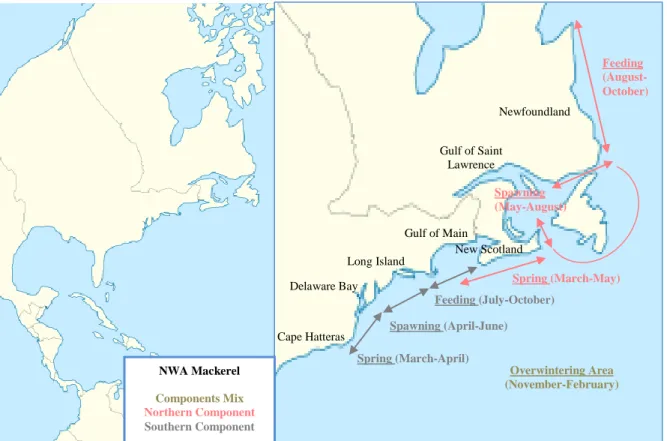
Figure 1.3 NWA mackerel components distribution ...8

Figure 3.1 Scomber scombrus individuals from Matosinhos collected at 16 of January 2018 (personal photograph) ...14

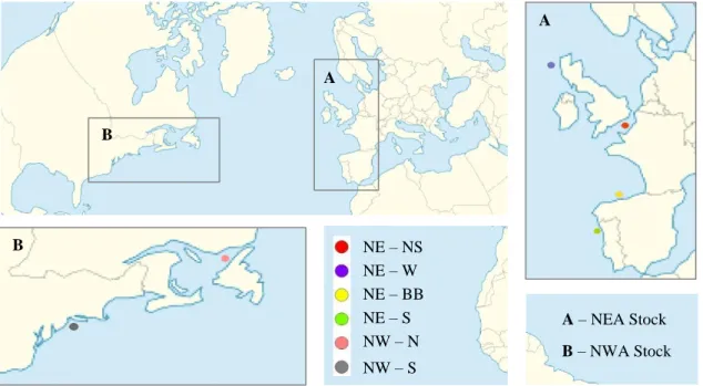
Figure 3.2 Scomber scombrus sampling locations of the individuals collected from January to February 2018 (A - NEA stock; B- NWA stock) ...14

Figure 3.3 3 year old Scomber scombrus left and right otoliths, respectively (individual from Bay of Biscay with a TL of 30 cm). See on lefth otolith the transduced bands numbered ...15

Figure 3.4 Right otolith sagittal photograph and the corresponding binary digital image (individual from Bay of Biscay collected at 24 of February 2018 with a TL of 30 cm) ...16

Figure 3.5 EFD Output - Otolith Shape Contour of the 1st Principal component (31% cumulative significance) and of the 14th Principal component (95% cumulative significance), respectively. 17 Figure 4.1 Canonical analysis of principal components (CAP) of the otolith shape signature (Shape Indices and Elliptic Fourier Descriptors analysis) for all the sampling locations (A), for the NEA stock (B) and for the NEA stock without NE-BB location (C) ...24

Figure 4.2 Mean ± SE Element:Ca concentration values for the sampling locations. In Element:Ca* there were significant differences between the NEA and NWA stocks (ANOVA, p < 0.05). For each Element:Ca, NEA sampling locations sharing the same letter do not show any statistical difference (Tukey, p > 0.05). For each Element:Ca, NWA sampling locations sharing the same number do not show any statistical difference (ANOVA p > 0.05) ... 26-27 Figure 4.3 Mean ± SE Isotopic Ratio concentration values for the sampling locations. In Isotopic Ratio* there were significant differences between the NEA and NWA stocks (ANOVA, p < 0.05). For each Isotopic Ratio, NEA sampling locations sharing the same letter do not show any statistical difference (Tukey, p > 0.05). For each Isotopic Ratio, NWA sampling locations sharing the same number do not show any statistical difference (ANOVA p > 0.05). ...27

(12)

viii

Figure 4.4 Canonical analysis of principal components (CAP) of the otolith chemical signature

(elemental and isotopic analysis) for all the locations (A), for the NEA stock (B) and for the NEA stock without NE-BB location (C) ...29

Figure 4.5 Canonical analysis of principal components (CAP) of the otolith shape and chemical

signatures (combined) for all the locations (A), for the NEA stock (B) and for the NEA stock without NE-BB (C). ...31

Index of tables

Table 3.1 Samples selected for the following analysis and respective sample size (N), fish total

length (TL), otolith length (OL) and otolith mass (OM). Values are presented as mean ± SE ...16

Table 3.2 Formulas used to obtain the otolith shape indices (Tuset et al., 2003). ...17

Table 4.1 Mean ± SE otolith Elliptic Fourier Descriptors (EFD) values for the sampling

locations. In EFD* there were significant differences between the NEA and NWA stocks (ANOVA, p < 0.05). For each line (EFD) NEA sampling locations sharing the same letter do not show any statistical difference (Tukey, p > 0.05). For each line (EFD) NWA sampling locations sharing the same number do not show any statistical difference (ANOVA p > 0.05) ...22

Table 4.2 Mean ± SE otolith Shape Indices (SI) values for the sampling locations. In SI* there

were significant differences between the NEA and NWA stocks (ANOVA, p < 0.05). For each line (SI) NEA sampling locations sharing the same letter do not show any statistical difference (Tukey, p > 0.05). For each line (SI) NWA sampling locations sharing the same number do not show any statistical difference (ANOVA p > 0.05) ...22

Table 4.3 The leave-one-out reclassification matrix of the otolith shape signature (Shape Indices

and Elliptic Fourier Descriptors analysis) for both stocks, NWA stock, NEA stock and NEA stock without NE-BB location ...23

Table 4.4 The leave-one-out reclassification matrix of the otolith chemical signature (element

and isotopic analysis) for both stocks, NWA stock, NEA stock and NEA stock without NE-BB location ...28

Table 4.5 The leave-one-out reclassification matrix of the otolith shape and chemical signatures

(13)

ix

List of abbreviations

ANOVA: One-way analysis of variance

ANCOVA: One-way analysis of covariance

CAP: Canonical analysis of principal coordinates

CI: Circularity

EFD: Elliptic Fourier Descriptors EL: Ellipticity

FAAS: Flame atomic absorption spectrometer

FF: Form Factor

IRMS: Isotope ratio mass spectrometry NEA: North Eastern Atlantic

NE-S: North Eastern Southern component

NE-BB: North Eastern Bay of Biscay NE-W: North Eastern Western component

NE-NS: North eastern North Sea component

NWA: North Western Atlantic

NW-N: North Western Northern component

NW-S: North Western Southern component

OA: Otolith Area OL: Otolith Length OM: Otolith Mass OP: Otolith Perimeter OW: Otolith Width

PERMANOVA: Permutational multivariate analysis of variance RE: Rectangularity

RO: Roundness

SB-ICP-MS: Solution based inductively coupled plasma mass spectrometry SI: Shape Indices

SE: Standard Error

TAC: Total Allowable Catch TL: Total Length

(14)

1

1. Introduction

1.1. Fisheries stock assessment

A fish stock is a semi-discrete group of fish with definable characteristics that are assumed to be a homogeneous unit for fisheries management purposes (Begg and Waldman, 1999). Stock identification is an interdisciplinary field that involves the recognition of self-sustaining components within natural populations (Cadrin et al., 2005). To manage a fishery effectively it is important to know the identity of the stock structure of a species in combination with estimation of the degree of exchange between stock members since, in fisheries that can contain several stocks, each stock may have unique demographic properties and distinct responses to exploitation or rebuilding strategies (Begg, 1998; Begg et al., 1999; Cadrin et al., 2005). Failing to detect the population structure of exploited marine fish species by neglecting that a single stock could be replenished by multiple populations or that multiple stocks could belong to a single population can lead to local overfishing and severe stock decline (Ying et al., 2011). Because stock demographics and the degree of overlap in their spatial range for periods of time are difficult to simultaneously assess, they are often ignored, resulting in false apparent trends in fishery assessments (Cadrin et al., 2014).

Ocean circulation patterns, sea-floor topology and other geographic features provide opportunities for species isolation and differentiation, but most of the world’s oceans lack obvious barriers (physical and/or oceanographic) (Souza et al., 2006). Several fish species have developed extended pelagic larval stages and high migratory capabilities as larvae, juveniles and adults, resulting in widespread ocean dispersal, which reduce the potential for geographic differentiation between distant populations (Souza et al., 2006). In the North Atlantic, commercially important pelagic fish stocks undertake extensive seasonal migrations that are connected to local ecosystem regimes, however, with changing environmental conditions, the spatial and seasonal distribution and life history strategy of the species may vary over time (Trenkel et al., 2014). Furthermore, stock discrimination is imperative for the fisheries management in the North Atlantic, and stock structure information provides a basis for understanding the dynamics of fish populations (Begg, 1998; Begg and Waldman, 1999). Modern fisheries management is moving towards a precautionary approach to ensure a sustainable and rational use of the marine resources, but stock assessment models are mainly

(15)

2

based on a single unit stock assumption; however, this assumption is often violated by greater stock complexity (Begg et al., 1999).

1.2. Atlantic mackerel

Atlantic mackerel (Scomber scombrus) is one of the most abundant and widely distributed pelagic migratory fish species in the North Atlantic, mostly restricted to the cold and temperate coastal regions (Hamre, 1978; Villamor et al., 2004; Souza et al., 2006). It is highly abundant from Morocco to the North of Norway in the Northeast Atlantic and from North Carolina to the North of Newfoundland in the Northwest Atlantic (Sette, 1950; Jamieson and Smith, 1987).

Scomber scombrus belongs to the scombridae family that aggregates all mackerel and

tuna species which normally habit temperate waters (Collette and Nauen, 1983). Its entire life cycle is pelagic: eggs and larvae drift passively with the oceanic currents until being juveniles and adults with a great swimming capability that form large schools, resulting in a great capacity for dispersion (Lockwood, 1988; Jansen and Gislason, 2013). This species lacks swim bladder, meaning that individuals need to swim continually to prevent sinking, but unlike species with swim bladder, fish can change depth rapidly (DFO, 1997). This species is affected by changes in sea water temperature via growth and mortality rates, particularly during the larval stage, which will reflect in its migratory and seasonal distribution patterns (Ware and Lambert, 1985; TRAC, 2010). S. scombrus is sensitive to temperature both in terms of physiological and behavioural responses and timing of migration and spawning, standing between minimum temperatures of about 5-6ºC and maximum of 15-16ºC; it can change very easily to shallower or deeper depths in

(16)

3

the water column according to their needs; and increases swimming speeds at low temperatures (Sette. 1950; Overholtz and Anderson., 1976; Studholme, 1999; Iversen, 2004). As juveniles they are opportunistic feeders, using both filter and biting behaviour to capture small crustaceans, pelagic fish and invertebrates; as adults the diet includes a variety of planktonic organisms (Studholme., 1999). Predation of this species is the largest component of natural mortality, with a large variety of predators such as larger fish, marine mammals and seabirds (Overholtz., 1991; Overholtz and Waring, 1991). Mackerel plays a key ecological role in oceanic and coastal ecosystems and supports one of the most valuable commercial fisheries in the North Atlantic (Trenkel et al., 2014).

Scomber scombrus is a fast growing fish species which begin to mature at age 2. being

generally fully mature at age 3; they are multiple spawners and the onset of spawning may be triggered by warm water temperatures (ranging between 13 and 15ºC) that ensure eggs hatch during periods of high zooplankton abundance (ICES, 1993; Studholme, 1999). The adults could reach a maximum length of 70 cm and 3 kg of weight, but these large sizes seem to be decreasing due to overfishing, with maximum sizes being around 60 cm and 2 kg at present (Navarro et al., 2012). The schools of mackerel tend to be composed of identical sized fish because of the close relationship between fish length and swimming speed (increasing with length) (DFO, 1997). Larger and older fish are the first to arrive to the spawning grounds followed by successively smaller individuals, by the end of the spawning season only the younger fish remain (Lockwood et al., 1981). Males mature earlier than females, but spawning ends at about the same time for both sexes (the testes seemed to develop earlier, but slower, than the ovaries) (Eltink, 1987). There is no evidence that migration to the spawning areas is carried out at different timesfor males and females (Villamor et al., 2004). Juveniles recruit in nearshore areas along the spawning grounds and the combination of early juveniles originating from all these areas results in the final overall recruitment (Lockwood, 1988; Borja et al., 2002).

There are two stocks in the North Atlantic, the Western and Eastern stocks (NWA and NEA, respectively). It is considered that these stocks have no habitat connectivity, being confirmed by molecular and tagging studies: the presence of mitochondrial DNA differentiation suggest a restriction in gene flow at large spatial scales; and tagging studies showed no individuals from Eastern origin being caught in the Western side, or vice versa (Nesbø et al., 2000; Uriarte and Lucio, 2001; Iversen, 2002; Tenningen et al., 2011). Atlantic mackerel´s

(17)

4

stocks are divided in five spawning components, two in the North Western Atlantic (NWA) and three in the North Eastern Atlantic (NEA) (Sette, 1950; ICES, 1996). Geographic distances separate the many grounds of the regional components of mackerel and although it was thought that they followed predictable migration patterns and spawned at regular times and places this does not necessarily occur (Jamieson and Smith, 1987; Jansen and Gislason, 2013). Through the years many interpretations on the mackerel migration and geographic distribution have been done because of its spatial-temporal dynamics due to environmental variations, resulting in lack of concrete knowledge on how these populations are structured (Sette, 1950; Jamieson and Smith, 1987; D’Amours and Castonguay, 1992; Iversen, 2002; Overholtz et al., 2011; Astthorsson et al., 2012; Radlinski et al., 2013; Jansen, 2016).

1.2.1. NEA population

The North Eastern Atlantic (NEA) stock, in terms of fisheries management, is composed of three spawning components: North Sea Component (ICES areas IIIa and IV), Western Component (ICES areas VI, VII and VIII) and Southern Component (ICES areas IX, X and subarea VIIIc), with the North Sea, Celtic Sea and Bay of Biscay as the main spawning grounds, respectively (Hamre, 1980; ICES, 2017). The latitudinal propagation of spawning reflects the increase of sea surface temperatures in the spring, as the migration from the spawning areas follows the Warm Shelf Edge current (Eltink, 1987; Reid et al., 1997). Spawning happens from February to May in the Southern component, March to July (with a peak in May) in the Western component and June to August (with a peak at the end of June) in the North Sea (Hamre, 1980; Iversen, 1981, Jorge et al., 1982). Fish after spawning in the Southern area migrate northwards, mix with the Western component and enter in the Norwegian Sea for the feeding period where they meet with the North Sea component (Uriarte and Lucio, 2001). Mackerel generally remain in the feeding area until the end of autumn, after which the individuals return south to their overwintering grounds around the North of the British Isles and then migrate back to their spawning grounds in the first half of the year (Punzón and Villamor, 2009; ICES, 2011). The onset of the spawning migration is determined by the rising temperatures in the wintering area, and higher temperatures are related with an early spawning season (Hamre, 1980). Furthermore, the southern pre-spawning migration pattern of the Atlantic mackerel seems to be directed towards areas with low turbulent mixing at spawning time, providing a “stable environment“ for egg and larval survival

(18)

5

as it seems that the turbulence conditions of pre-spawning and spawning periods have the largest influence on the success of recruitment (Borja et al., 2002; Jansen, 2013).

The first establishment of the NEA spawning components was based on tagging experiments and, since then, other natural tags (e.g. parasite infestations, protein polymorphisms, juvenile growth patterns in otoliths, age composition, length at age, genetics) where used to differentiate them, but until now none really supported their spatial isolation (Hopkins, 1986; Jamieson et al., 1987; Dawson, 1991; Nesbø et al., 2000; Jansen and Gislason, 2013; Levsen et

al., 2017). The existence of the Southern component, which aggregates mackerel from the

Iberian Peninsula, is recent (ICES, 1996). Before that, the individuals from the Southern and Western component were considered to belong to one single component, the Western component alone. Furthermore the mixing of individuals from the southern and western areas throughout most of the year and their cohabitation in the western spawning grounds still raise doubts on the reliability of the assumption of separate spawning components in these two areas (ICES, 2001). The fact that the egg distribution of the Southern and Western components overlaps in the Bay of Biscay, makes it very difficult to define the Northern border of the Southern component and the southern border of the Western component (Iversen, 2002).

Figure 1.2 NEA Mackerel components distribution.

Spawning (June-August)

Overwintering area (Until the end of the year)

Feeding area (Autumn)

NEA Mackerel Components Mix

North Sea Component

Western Component Bay of Biscay Southern Component Spawning (February-May) Spawning (March-July) Overlapping area

(19)

6

1.2.2. NEA stock fishery

The stock size and migration pattern of the different spawning components of mackerel in the NEA have changed over time and, as a consequence, also the fishery and its management (Iversen, 2002). This species is widely distributed through the ICES areas and supports one of the most valuable European fisheries, with an estimated catch of 1 155 944 tons in 2017, and world fisheries, being ranked 9th in 2014 (FAO, 2016; CES, 2018). Mackerel is caught by a variety of fleets ranging from open boats using hand lines and purse seines on the Iberian coasts to large freezer mid-water trawlers in the Northern Areas (ICES, 2011). Migration routes are usually known and exploited by local fisheries (Punzón and Villamor, 2009). In the beginning of each year, the stock is mainly fished in the spawning grounds west of the British Isles, France, Spain and Portugal (about ¼ of the total catch); in the summer and autumn, mainly in the north into the Norwegian Sea and around the south of Iceland (about ½ of the total catch); and in the end of the year, the fishery is concentrated around the Shetland Islands in the overwintering area, when the components are migrating back to their spawning grounds (about ¼ of the total catch) (Hannesson, 2012; ICES, 2018).

The Western component is considered to be the largest and the North Sea is considered overfished since 1970´s (ICES, 2011). The collapse of mackerel in the North Sea in the late 1960´s was most likely driven by very high catches and associated fishing mortality; however the lack of recovery is probably associated with unfavourable environmental conditions that led the mackerel to spawn in Western waters instead of in the North Sea (ICES, 2018).

Over the last few years there have been dramatic changes in the mackerel fishery in the Northeast Atlantic. In 2007 the mackerel changed its migratory habits and appeared in large quantities in the Icelandic economic zone, and in 2013 the first records in the Arctic waters of Svalbard were registered (Hannesson, 2014; Berge et al., 2015). The feeding distribution has apparently expanded northward and westward probably related to co-occurring factors, such as a gradual increase in temperature, changes in the feeding conditions, competition with other major pelagic fish stocks in the area, and the relatively good status and age/size structure of the mackerel stock (Astthorsson et al., 2012). Climate change affects zooplankton abundance and distribution, as well as ocean temperature and ocean circulation patterns (Astthorsson and Gislason, 2003). The increasing water temperature opens new and different feeding grounds and in contrast to species with restricted dispersal, migratory species, such as mackerel, might be less

(20)

7

constrained in responding to climate change (ICES, 2011; Hughes et al., 2014). Especially when, at the time, there were signs of an increased abundance of mackerel with higher recruitment, year-classes and large cohorts suggesting that the expansion of the mackerel stock might also been density driven (Hannesson, 2012; ICES, 2013; Jansen, 2016).

The appearance of mackerel in Iceland has led to some disagreements between the parties involved in its management (Norway, European Union, Faroe Islands North East Atlantic Fisheries Commission), since Iceland did not agreed with the total allowable catch (TAC) offered by the traditional partners and unilaterally set a quota for itself, taking about 20% of the total catch in 2008 (Hannesson, 2012). In response, the Faeroe Islands dropped out of the mackerel agreement, since they thought that their share was small compared to the Icelandic catches (Hannesson, 2014). As result the management agreement was broken, and in 2010 the share of catches taken in the area which covers parts of the Icelandic, Faroese, and Norwegian economic zones, increased to unprecedented levels (Berge et al., 2015). Currently there is no agreement on a management strategy covering all parties fishing mackerel (ICES, 2018). In 2014, three of the Coastal States (The EU, Faroes and Norway) agreed on a Management Strategy for 2015 and the subsequent five years; however, the total declared quotas taken by all parties since 2015 have greatly exceeded the TAC advised by ICES and spawning stock biomass has been decreasing since 2016 (ICES, 2018).

1.2.3. NWA population

The North Western Atlantic (NWA) mackerel is found from North Carolina to Newfoundland and has two spawning components (Sette, 1950). The Northern component that spawns mainly in the Gulf of St. Lawrence, along the Coast of New Scotland and possibly on the Grand Banks of Newfoundland (from May to August); and the Southern component that spawns from the Mid-Atlantic Bight to the Gulf of Maine (from April to June) (Sette, 1950; Berrien, 1982; DFO, 1997). During spring and summer Atlantic Mackerel is found in inshore waters, and from late fall through winter they co-occur deeper in warmer waters at the edge of the continental shelf in the Mid-Atlantic Bight (DFO, 2012). After the overwintering period, the Southern component moves inshore inhabiting the waters between Cape Hatteras and Delaware from March to April, thereafter migrating North to spawn, after which they move North again to feed in the coastal waters of the Gulf of Maine where they stay until autumn (Ware and Lambert,

(21)

8

1985). The Northern component moves shoreward from the Continental Shelf off New England and southern New Scotland in the spring and migrates north to spawn; after spawning the schools disperse north to feed around the Newfoundland coast (Ware and Lambert, 1985). The Southern contingent stays farther inshore, the northern component stays more offshore, but the two may cross paths in late spring or late summer in southern New England and in the Gulf of Maine (Sette, 1950; Studholme, 1999). Similarity to the NEA stock, no significant genetic differences have separated the two components (Souza et al., 2006). Also, they seem to be very similar in terms of migratory behaviour change response when faced with different environmental conditions (Overholtz et al., 2011; Radlinski et al., 2013; McManus et al., 2016).

1.2.4. NWA stock fishery

Atlantic mackerel is part of an important Northwest fishery, the stock is commercially exploited by the USA and Canada, and quota regulated by both (NOAA and DFO respectively) (TRAC, 2010). The two components are managed as a single stock (Northwest Atlantic Fisheries Organization, NAFO, Subareas 2-6) because of the important fishery in their overwintering area

Figure 1.3 NWA Mackerel components distribution. NWA Mackerel Components Mix Northern Component Southern Component Spring (March-April) Spawning (April-June) Feeding (July-October) Cape Hatteras Delaware Bay Long Island Gulf of Main Spring (March-May) Feeding (August-October) Gulf of Saint Lawrence Overwintering Area (November-February) Newfoundland Spawning (May-August) New Scotland

(22)

9

offshore along the edge of the Continental Shelf, from Stable Island to Long Island, where they co-occur (Ware and Lambert, 1985; TRAC, 2010). Both populations are also exploited on their spawning grounds in a summer and in a spring fisheries (Overholtz, 1991).

Both US and Canada landings (1/2 of the total catch reportedly taken from each

component) have been decreasing since 2006 and it is now at a point never seen before, with landings being more than 10 times less from what they used to be (decreased from around 110 000 tons to 10 000 tons) (DFO, 2017). As for the NEA stock, NWA stock distribution has been shifting (e.g, northern and eastern) due to global warming (Overholtz et al., 2011; McManus et

al., 2017). Also, recently, Atlantic mackerel have been seen in more inshore shallower waters of

the Northeast Continental Shelf during winter, possibly owing to a general warming pattern in the region (NEFSC 2006; Overholtz et al., 2011; Radlinski et al., 2013). The availability of the fish to the fishery seems to be highly affected by environmental changes from year to year, since their migration behaviour change in order to follow the optimal conditions (Overholtz, 1991). The stock decline is being caused by levels of fishing mortality much higher than previously sustainable levels, and is also thought that is currently in an overfishing situation (DFO, 2014; Plourde et al., 2015). Besides the decreasing trend in catch through the years, other indicators such as the absence of older individuals and recent poor recruitment are solid indicators of a stock that is being overfished and, additionally, it is near its historical minimum (Duplisea and Grégoire, 2014). For the Northern component, a study revealed the possibility of being at its lowest biomass, since the annual catch was being well below the TAC (Grégoire and Beaudin, 2013). Furthermore, there are large and unaccounted catches in recreational and bait fisheries in Canada, since the commercial fishery (primarily seine) is obligated to declare landings but bait and recreational fisheries do not always need to report catches (Duplisea and Grégoire, 2014; VanBeveren et al., 2017). Though there is no clear handle on the magnitude of unregulated recreational and bait fishery catches, they may sum to more than the reported commercial fishery catch (Duplisea and Grégoire, 2014). The bait fishery is mainly to bait American lobster and snow crab pots, and mackerel angling is a common summer activity on the wharves, rocky points and recreational boats in Atlantic Canada (VanBeveren et al., 2017). As for the Southern component (with a fishery supported by midwater and bottom trawls) the Atlantic mackerel supplied an early-spring recreational fishery along the nearshore region of the Middle Atlantic Bight (when the Southern component moves inshore from the wintering grounds); however, this

(23)

10

fishery began to decline in the late 1970´s and early 1980´s (Overholtz, 1991). Landings of Atlantic mackerel in the Middle Atlantic Bight further declined from the 1990´s and, beginning in 2005, the U.S. commercial fishery began to experience difficulty in locating large schools of Atlantic mackerel (NEFSC 2006).

1.3. Otoliths as natural tags

1.3.1. Otolith chemical signature

Otoliths have several specific characteristics that make them excellent natural markers of fish habitat and valuable tools for studies of fish life history and movements (Campana and Thorrold, 2001). They are biogeochemical structures deposited continuously throughout the fish life that grow by the addition of calcium carbonate and by the successive uptake of chemical elements present in the surrounding seawater in a layered manner that preserves the timing of deposition (Thresher, 1999; Elsdon and Gillanders, 2003). Otoliths are accretionary structures located within the inner ear of teleost fish, composed primarily of aragonite deposited on a proteinaceous matrix, accreted within a gel-filled endolymph and thus are isolated from direct exposure to the external water (Campana and Neilson, 1985) That, along with low ratios of surface area to volume and a relatively large size (mm to cm) and being metabolically inert, makes them less vulnerable to post-depositional chemical and structural modification than many other types of biogenic carbonate (Thorrold et al., 1997; Ghosh et al., 2007).

The uptake of elements into the growing structures usually reflects the aquatic environment where the fish lived (Campana et al., 2000). Any relationship between water composition and otolith chemistry will be determined by the kinetics of ion transport from water to the precipitating surface, but will also be a function of the mechanism by which the trace elements are incorporated into otolith aragonite (Bath et al., 2000). The physico-chemical properties of the environment (e.g., water composition, temperature, pH and salinity), fish physiology (e.g., age, growth and metabolism), upwelling phenomena and feeding regime are among the factors that can influence the potential incorporation of elements in the otoliths (Campana et al., 2000; Gao et al., 2001; Elsdon and Gillanders, 2002; Elsdon et al., 2008). The concentration of certain elements in the water is known to have a higher effect on the chemistry of the otoliths; the use of combined elemental signatures is likely to enhance the interpretations made (Thorrold et al., 1997; Elsdon and Gillanders, 2003; Elsdon and Gillanders, 2004).

(24)

11

Stock discrimination is based on the hypothesis that fish inhabiting different water bodies will incorporate elements into their calcified structures, which combine to form a unique and spatially distinct chemical signature that reflects the length of time that the fish occupied a particular water body (Elsdon et al., 2008; Daros et al., 2016). The most common application of stock identification is discriminating between separate populations that were previously assumed to be a single one, through quantitative analysis of the micro constituents and trace elements in otoliths which can provide information on population structure, habitat connectivity and the movements of individual fish (Campana et al., 2000; Higgins et al., 2013; Correia et al., 2014; Carvalho et al., 2017). A more robust application of whole otolith fingerprints might be one which is targeted at questions of stock mixing or for tracking stock migrations, in which the fingerprints are used as biological tracers of pre-defined groups of fish over short periods of time (Campana et al., 1995).

Owing to the potential value of otolith microchemistry to fisheries ecology and management, numerous analytical techniques have been adapted to quantify the elemental concentrations of otoliths (Campana et al. 1997; Campana, 1999; Thresher, 1999). One technique of growing importance and widespread use is the inductively coupled plasma mass spectrometry (ICP-MS), probably related to its extremely low detection limits which allow for a wide range of elements to be precisely and accurately quantified (Campana et al. 1997; Campana, 1999; Thresher, 1999). Choosing the exact instrument of analysis is important because of the elevated detection limits that might arise from small otolith mass or contamination during storage, preparation and handling, which can prevent the chemical detection by the process (Elsdon and Gillanders, 2003; Ludsin et al., 2006).

1.3.2. Otolith shape signature

In the variety of techniques used at present for the study of fish population structure (e.g. genetics, parasitic fauna, body morphology) otolith geometric morphometric is a relatively new tool to fisheries research and it seems promising as a means of enabling researchers to cheaply and quickly categorize fish to individual stocks based on variations in otolith form, most commonly size and shape (Tracey et al., 2006; Agüera and Brophy, 2011; Tuset et al., 2013). The shape of the otolith would appear to be an ideal natural marker for fish populations, as it is species specific and less affected in growth than fish body growth due to short-term

(25)

12

environmental changes (Hopkins, 1986; Campana and Casselman, 1993). Also, measurements made on otoliths have the advantage of being unaffected by short-term changes in fish condition or by preservation, as long as acidic preservatives are avoided (Campana and Casselman, 1993).

Otoliths may show characteristics that are stock specific since geometric outline methods quantify boundary shapes so that patterns of shape variation within and among groups can be evaluated (Cadrin and Friedland, 2005; Pothin et al., 2006; Moreira et al., 2019; Soeth et al., 2019). Although sagittal otoliths have certain morphological features that are laid down early in the ontogeny of the fish, some characteristics (e.g. sulcus area, depth of the sulcus and the sulcus area: otolith area ratio) vary according to ecological factors such as fish length, geographic area, depth, conspecific abundance, food regime, chemical and physical characteristics of the environment (Lombarte and Lleonart 1993; Tuset et al., 2003; Cardinale et al., 2004).

Sagittae, the most used and bigger otolith’s pair, are generally laterally compressed, elliptical on their sagittal plane, compressed on their internal-external axis and present a main axis of growth oriented in the anterior-posterior direction; most morphometric studies of otoliths have concentrated on these characteristics, evaluating size dependent measurements made on their sagittal plane and on size independent shape analysis of contour (Ponton, 2006). The size dependent variables recorded from the otolith will allow for different shape indices to be accounted like, roundness, circularity, rectangularity, ellipticity and eccentricity (Tuset et al., 2003; Ponton, 2006). The size independent measurements, most known as Fourier descriptors, are mathematically defined as a series of sinusoids (harmonics) that together give information on the outline of a shape (Gastonguay et al., 1991). This technique is considered useful because of the magnitude of the amplitude associated with each harmonic, indicating the contribution of that particular harmonic to the total form, each of them adding increasing detail to the description of the shape (Campana and Casselman, 1993; Ponton, 2006). This method represents a precise way of accommodating significantly complex shapes and efficiently capturing outline otolith information (Tracey et al., 2006).

Otolith shape analysis is an efficient tool to assess the stock identity and/or population structure, reflecting the areas which the fish inhabits (Farias et al., 2009; Moreira et al., 2019; Soeth et al., 2019). Age, sex, fish length and year class usually have effect on otolith shape Simoneau et al., 2000; Cardinale et al., 2004); and, even though for this species sex has showed not to influence, the otolith shape, age and year class seem to have great effect on shape

(26)

13

variability and they must be accounted for (Gastonguay et al., 1991). Several environmental factors can make the pattern of mackerel growth variable in time and place so length distributions for age assignation is not recommendable and every individual should be aged by otolith reading (ICES, 2001). Also, comparing otoliths of fish from different size ranges can lead to wrong interpretations about the population structure if these differences are not accounted and techniques must be used to control the effect of fish otolith size on otolith shape (Campana and Casselman, 1993; Simoneau et al., 2000; Ponton, 2006; Mapp et al., 2017).

2. Objectives

Atlantic Mackerel seems to have a complex population structure since its movement patterns and spatial distribution keep changing due to environmental conditions, which results in a fishery that is somewhat uncertain. It becomes urgent to truly understand the differentiation between the spawning components for a correct management of the different stocks. To complement past studies on the population structure, the hereby work tested alternative natural tags allowing the use of a multidisciplinary approach than can help unravel mackerel population dynamics. The purpose of this work was to assess the utility of otolith chemistry and shape analysis to provide information about the population structure, habitat connectivity and migration patterns of S.

scombrus. The obtained new findings will be made available for decision makers and fisheries

agencies to improve the mackerel management in the North Atlantic. Specifically, we aimed to: 1. examine the variations of whole otoliths chemistry (entire life-history prior to capture)

and shape characteristics between S. scombrus from the NEA and NWA stocks and to evaluate the differences between components within each stock;

2. investigate whether there is a discontinuity or not between Southern and Western components of the NEA stock, including a sampling location in the Bay of Biscay.

3. Methodology

3.1. Fish collection

A total of 300 individuals were collected (50 from 6 different locations) from local fisheries or boat surveys (in general, with seiners and trawlers) from January to February 2018. An effort was made to choose adult individuals from specific component occurrence areas and with similar

(27)

14

length. Length (total length, TL, 0.1 cm) and weight (total mass, TM, 0.1 g) of each individual were measured.

Fish samples came from: NWA Northern Component - Corner Brook, Newfoundland, Canada; NWA Southern Component - Belford, New Jersey, USA; NEA Southern Component - Matosinhos, Porto, Portugal; NEA Bay of Biscay (Part of the Southern and Western Components) - Gijon, Oviedo, Spain; NEA Western Component - Saint Kilda, Scotland, United Kingdom; NEA North Sea Component - Isle of Wight, London, United Kingdom (Figure 3.2).

Figure 3.1 Scomber scombrus individuals from Matosinhos collected at 16 of January 2018

(personal photograph).

Figure 3.2 Scomber scombrus sampling locations of the individuals collected from January to

February 2018 (A - NEA stock; B- NWA stock).

A – NEA Stock B – NWA Stock NE – NS NE – W NE – BB NE – S NW – N NW – S A B A B

(28)

15

3.2. Otoliths extraction, storage and age reading

Each pair of otolith was extracted with plastic forceps to avoid metallic contamination, cleaned with ultrapure water, until all organic tissue was removed, air dried and storage in labelled Eppendorf’s tubes.

For mackerel age estimation an existent standard protocol was followed (ICES, 2010). Otoliths were viewed with a stereomicroscope (Meiji Techno, EMZ-13TR) with a reflected light and under black background, sulcus faced down, and immersed in a clearing agent (ethanol and glycerol, 1:1) to enhance their annuli transparency during reading. The annual growth pattern is well defined on the otolith with clear contrasting opaque and translucent bands. The date of birth is assumed to be 1st January and the fish is assigned to a year class on this basis. One opaque zone and one translucent band constitutes one year of growth (annulus). For counting purposes the opaque increment should be continuous around the otolith (the increment should be visible in at least two areas). For mackerel caught in the 1st semester of the year, all translucent increments and the translucent edge are counted. The translucent edge is always counted as one winter ring, even if nothing or very little is visible. Two independent and experienced observers made two blind readings of each otolith and concordance percentage was calculated (% concordance = number of coincident reads/number of total reads) to determine reliability of age estimates. Only fish with 100% concordance of age readings were used.

Figure 3.3 3 year old Scomber scombrus left and right otoliths, respectively (individual from

Bay of Biscay collected at 24 of February 2018 with a TL of 30 cm). See on left otolith the translucent bands numbered.

1 mm 1

2 3

(29)

16

The majority of the samples of all the places were 3 years old so that was the age chosen to analyse. Regarding this, it was possible to select 30 individuals from each location for the analysis (with a total of 180 individuals analysed). Furthermore right otoliths were used for the elemental and shape analyses and the left otoliths for the isotopic analysis (Table 3.1.)

Location N Code TL (cm) OL (mm) OM (mg)

NEA Southern Component 30 NE-S 32.6 ± 0.3 4.21 ± 0.05 2.50 ± 0.05

NEA Bay of Biscay 30 NE-BB 29.6 ± 0.3 3.97 ± 0.05 2.31 ± 0.06

NEA Western Component 30 NE-W 32.9 ± 0.2 3.99 ± 0.05 2.37 ± 0.06

NEA North Sea Component 30 NE-NS 28.1 ± 0.2 3.93 ± 0.05 2.31 ± 0.06

NWA Northern Component 30 NW-N 38.4 ± 0.4 4.50 ± 0.04 3.23 ± 0.06

NWA Southern Component 30 NW-S 29.3 ± 0.4 3.98 ± 0.07 2.14 ± 0.06

3.3. Otolith shape analysis

3.3.1. Shape Indices

Orthogonal two-dimensional digital images of the sagittal otoliths were captured using a stereomicroscope (Meiji Techno, EMZ-13TR) coupled with a USB digital camera (Olympus, SC30) at 1.5 X magnification with the analySIS getIT software (Moreira et al., 2019). Right otoliths were all photographed in the same position, with reflected light and dark background. The photos quality was improved in the paint.NET (v. 4.0.21) program, in order to maximize the differentiation between the otolith and the background and to create a binary image.

Table 3.1 Samples selected for the following analysis and respective sample size (N), fish

total length (TL), otolith length (OL) and otolith mass (OM). Values are presented as mean ± SE.

Figure 3.4 Right sagittal otolith photograph and the corresponding binary digital image

(individual from Bay of Biscay collected at 24 of February 2018 with a TL of 30 cm), respectively.

(30)

17

Binary otolith images were measured using the program ImageJ (v. 1.50) (Rasband, 2009) to assess the morphometric size parameters, otolith length (OL, mm), otolith width (OW, mm), otolith area (OA, mm2), and otolith perimeter (OP, mm). With these variables is possible to calculate and assess the Shape Indices (SI) (Form factor, Roundness, Ellipticity, Circularity and Rectangularity) that were used to evaluate and compare the otoliths shape (Tuset et al., 2003).

Shape Indices (SI) Formula

Form Factor (FF) (4𝝅OA)/OP2 Roundness (RO (4OA)/(𝝅OL2)

Ellipticity (EL) (OL−OW)/(OL+OW) Circularity (CI) OP2/OA Rectangularity (RE) OA/(OL×OW)

3.3.2. Elliptical Fourier Descriptors

The Elliptic Fourier analysis fits a closed curve to an ordered set of data points and then decomposes the contour into a sum of harmonically related ellipses (Kuhl and Giardina, 1982). The program Shape (Version 1.3) was used to extract the otolith contour and to determine the number of Elliptic Fourier Descriptors (EFD) required to adequately describe the otolith outline. A level of 95% of accumulated variance was used to select the minimum number of harmonics (each harmonic characterised by 4 Fourier descriptors, a, b, c and d) (Ferguson et al. 2011). The first 5 harmonics reached >95% of the cumulative power, excluding coefficients b5, c5 and d5, indicating that the otolith shape could be adequately explained by 17 Fourier coefficients. After normalization to the first harmonic (EFD invariant to otolith size), the first three coefficients (a1, b1 and c1) were constant and excluded (Iwata & Ukai 2002; Pothin et al., 2006), and 14 Fourier descriptors (17-3) used in the subsequent analyses.

(31)

18

3.4. Otolith chemical analysis

3.4.1. Otoliths pre-treatment

Even though the glycerol, from the clearing solution for the age reading, would take 1 to 2 months of immersion to enter otoliths, otoliths pairs were rinsed in ethanol and brushed in Milli-Q water to remove any superficial glycerol contamination (Campana, 1999; Campana et al., 2003). Thereafter otoliths were cleaned and decontaminated in an ultrasonic cleaner for 5 min in ultrapure water (Milli-Q water) to remove any adherent biological tissues, followed by immersion in 3% analytical grade hydrogen peroxide (H2O2) for 15 min, to remove any

remaining biological residues (Correia et al., 2011). Otoliths were immersed in ultrapure 1% nitric acid (HNO3) solution for 10 s to remove any superficial contamination, followed by a

triple-immersion in Milli-Q water for 5 min to remove the acid (Rooker et al., 2001). The otoliths were stored in new decontaminated Eppendorf micro centrifuge tubes, and allowed to dry in a laminar flow fume hood (Patterson et al., 1999; Daros et al. 2016). The decontaminated otoliths were weighed on an analytical balance (otolith mass, OM, 0.001 g).

3.4.2. Elemental analysis

Right whole otoliths were dissolved for 15 minutes in 60 μL of ultrapure HNO3 and diluted with

Milli-Q water to a final volume of 3 mL [2% of HNO3 (v/v) and 0.02% of TDS (m/v)]. The

solution was stirred with a vortex and sent to the laboratory (Correia et al., 2011).

Multi-elemental analysis was performed by SB-ICP-MS using an iCAPTM Q (Thermo Fisher Scientific, Bremen, Germany) instrument equipped with a concentric glass nebulizer, a Peltier-cooled baffled cyclonic spray chamber, a standard quartz torch and a two-cone interface

Figure 3.5 EFD Output - Otolith Shape Contour of the 1st Principal component (31%

cumulative significance) and of the 14th Principal component (95% cumulative significance),

(32)

19

design (sample and skimmer cones). High-purity (99.9997%) argon (Gasin II, Leça da Palmeira, Portugal) was used as the nebulizer and plasma gas. The equipment control and data acquisition were made through the Qtegra software (Thermo Fisher Scientific, Bremen, Germany). To minimize the effect of any plasma fluctuations or different nebulizer aspiration rates among samples, Indium (115In) was monitored as internal standard. The limits of detection (LoD were calculated as the concentration corresponding to three times the standard deviation of 10 sample blanks. Only the 44Ca was analysed by FAAS - Flame Atomic Absorption Spectrometry instrument (Perkin Elmer, Überlingen, Germany). Otolith samples were analysed in random order to avoid possible sequence effects.

For quality control, precision and accuracy checks, the NRC otolith certified reference material FEBS-1 was also analysed (Sturgeon et al., 2005). Elemental concentrations determined in FEBS-1 were within the certified and indicative range, with a value of recovery >95%. The precision of replicate analyses of individual elements ranged between 3% and 4% of the relative standard deviation (RSD). Nine elements) were above the limit of detection (LoD mg/L): 44Ca (0.015 mg/L), 23Na (0.403 μg /L), 88Sr (0.079 μg /L), 7Li (0.002 μg /L), 26Mg (0.044 μg /L), 55Mn (0.019 μg /L), 59_{Co (0.006 μg /L),}60_{Ni (0.009 μg /L), and}137_{Ba (0.007 μg /L).}44

Ca provided the internal standard. Data were also collected for 9Be (0.004 μg /L), 52Cr (0.051 μg /L), 65Cu (0.022 μg /L), 66_{Zn (0.252 μg/L),} 82

Se (0.354 ug/L), 85Rb (0.024 μg/L), 75As (0.119 μg /L), 95Mo (0.006 μg /L), 111_{Cd (0.003 μg /L),}118_{Sn (0.005 μg /L),}121_{Sb (0.002 μg /L),}205_{Tl (0.002 μg /L),}209

Pb (0.001 μg /L) and 238_{U (0.0004 μg /L), but their concentrations were consistently below the limit}

of detection.

The trace elements concentrations, originally in μg element/L solution, were transformed to μg element/g otolith and finally to μg element/g calcium (Correia et al., 2011).

3.4.3. Isotopic analysis

δ18_{O and δ}13

C were analysed. Otoliths were crushed into a fine powder using a small mortar and pestle. The crushed powder (20–40 μg) was analysed for stable oxygen and carbon isotopic composition using an automated carbonate device (Kiel IV) connected to a Thermo Finnigan MAT 253 Dual Inlet Isotope Ratio Mass Spectrometer (IRMS). Otolith samples were analysed in random order to avoid possible sequence effects. In the carbonate, the otolith powder was reacted with phosphoric acid (H3PO4), the formed CO2 was purified by two traps and transported by

(33)

20 vacuum to the IRMS, where δ18_{O and δ}13

C were measured against a calibrated reference CO2 gas. Each sequence was carried out with external NBS19 (for both δ18_{O and δ}13

C) and NBS18 (for δ13

C only) reference standards, and in- house NFHS1 standard (for both δ18O and δ13C) to check for drift. Test measurements were done to check the homogeneity of one sample. Isotopic concentrations measurements (‰ VPDB) were guided and calculations done with Isodat 3.0 (Thermo Scientific) software. The reproducibility of all standards, standard deviation (SD), amounted to 0.1‰ and 0.06‰ for δ18_{O and δ}13

C, respectively.

3.5. Data analysis

To ensure that differences in otolith length and mass among locations did not confound any location specific differences in otolith shape or chemical analysis, the relationship between Shape Indices and otolith length (OL) (as covariate) and between Element:Ca concentrations and otolith mass (OM) (as covariate) was evaluated using analysis of covariance (ANCOVA) (Campana et al., 2000; Daros et al., 2016). EL and CL showed a positive relationship with OL (r² =0.530, n=180, p < 0.05; r² =0.410, n=180, p < 0.05, respectively), opposite to FF, RO and RE that showed a negative relationship with OL (r² =0.417, n=180, p < 0.05; r² =0.529, n=180, p < 0.05; r² =0.167, n=180, p < 0.05, respectively). Mg:Ca and Ba:Ca concentrations showed a negative relationship with OM (r² =0.417, n=180, p < 0.05; r² =0.529, n=180, p < 0.05, respectively). The variables affected by the respective covariate were corrected using the ANCOVA slope, the formula used to correct it was Vadj = V − (β × covariate), where Vadj is the adjusted sample value, V is the original sample value and β is the slope value (Campana and Casselman 1993; Cardinale et al. 2004; Ferguson et al. 2011). After the corrections, ANCOVA showed that the corrections were effective in removing the OM and/or OL effect in the data.

Prior to the rest of the statistical analysis, data were checked for normality (Shapiro–Wilk test, p > 0.05) and homogeneity of variances (Levene’s test, p > 0.05). These assumptions were met after log10 transformation of RO and RE in the shape analysis and Sr:Ca and Mn:Ca in the

chemical analysis.

All statistical analysis were applied to infer for differences between stocks (NEA vs NWA), differences between locations within each stock (NWA: NW-N vs NW-S and NEA: NE-NS vs NE-W vs NE-BB vs NE-S) and an additional analysis was performed to the NEA stock without the presence of the NE-BB location (NEA: NE-NS vs NE-W vs NE-S).

(34)

21

Univariate one-way analysis of variance (ANOVA) was used for each variable of the shape and chemical analysis. ANOVA was followed by a Tukey post-hoc test if significant differences were found (p < 0.05).

Multivariate canonical analysis of principal coordinates (CAP) based on Euclidian distances to examine the reclassification accuracy (leave-one-out cross-validation) was applied to the shape signature, to the chemical signature and to the shape and chemical signatures combined to observe grouping separation of the locations and the variables that most contributed for the discrimination. CAP was followed by a permutational multivariate analysis of variance (PERMANOVA) (p-values were generated using 9999 random permutations) to check for significant differences. Models found to be statistically significant were followed by permutational pairwise comparisons (p < 0.05).

All statistical analyses were performed using Systat (v. 12) and PRIMER 6+PERMANOVA software with a statistical level of significance (α) of 0. 05.

4. Results

4.1. Shape signature

Less than half of the EFD (a3, c3, a4, c4, d4 and a5) presented differences between the stocks (NEA vs NWA), but all SI differentiated them (ANOVA, p < 0.05) (Table 4.1 and 4.2). Regarding the NWA stock, NW-N and NW-S sampling locations did not show significant differences for any EFD (ANOVA, p > 0.05) but in contrast showed significant differences for all SI (ANOVA, p < 0.05) (Table 4.1 and 4.2). Regarding the NEA stock, essentially, NE-S differed from NE-W in 5 EFD (a2, a3, b3, b4, d4) (Tukey test, p < 0.05), as for SI none of the NEA sampling locations showed significant differences (ANOVA, p > 0.05) (Table 4.1 and 4.2). ANOVA and Tukey test results with and without the presence of NE-BB location presented identical results.