MASTERS IN FINANCE AND BUSINESS ECONOMICS
ASSET PRICING AND TEMPERATURE: AN ESSAY FOR BRAZIL
by
RICARDO FERRARO GILABERTE DA SILVA
Rio de Janeiro 2010
ASSET PRICING AND TEMPERATURE: AN ESSAY FOR BRAZIL
by
RICARDO FERRARO GILABERTE DA SILVA
Thesis submitted to the Fundação Getúlio Vargas Graduate School of Economics Examination Board as partial requirement for obtaining a Master’s Degree in Business Economics and Finance, under the direction of Professor Marcelo Verdini Maia.
Rio de Janeiro 2010
RICARDO FERRARO GILABERTE DA SILVA
ASSET PRICING AND TEMPERATURE: AN ESSAY FOR BRAZIL
Thesis submitted to the Graduate School of Economics at Fundação Getúlio Vargas as a partial requirement to obtain the Master’s degree in Finance and Business Economics.
Approved on 28/05/2010
Examination Board
Marcelo Verdini Maia IAG/PUC-RJ
Pedro Cavalcanti Ferreira EPGE / FGV
André Luiz Carvalhal da Silva IAG/PUC-RJ
Dedication
My beloved Samantha for her affection, companionship, understanding and support since the beginning of the journey, and at all times. Without you by my side, I wouldn´t have come this far;
To my father, my mother, my brother and sister, and my whole family for being my first mentors and humanists who have always inspired me;
To Prof. Marcelo Verdini Maia, for his continuous encouragement, and making me believe it would be possible to complete this project within the deadlines proposed, for the knowledge he shared and for his friendship;
To the professionals of IRB-Brasil Re insurance and reinsurance market, who believe in what is good in our country and our organizations. In particular, to the friends of the Treaty Department (GETRA), Luis Mario de Barros, Renata Trindade and the entire team whose invaluable help and understanding contributed to the conclusion of this thesis. To the friends of the Loss Adjustment Department, Francisco Magalhães, José Francisco, César Janine and Antonio Moussalem, with whom I had the opportunity to deepen my knowledge about claims processing and reinsurance, along with other areas; Claudio Crez, Manoela Cabo Márcia Lima, Uziel Oliveira, Sylvio Couto, Michelle de Pinho Viard, Osvaldo Nakiri, who have collaborated in developing this project, each one in their own way, through discussions on insurance and reinsurance, or through helping with data processing,
To all the teachers and colleagues at EPGE/FGV, for their teachings, examples, short conversations and the high level of conviviality and education. To Prof. Marcelo Pessoa for his special attention and the patience in addressing and answering so many questions; to Luiz Felipe Pires Maciel, Daniela Kubudi, Ilton Gurgel Soares, Vitor Souza Barros, Aline de Souza Cardoso, Ana Carolina Secchin Silva, the entire team of NC/EPGE and FGV employees; To the meteorology colleagues who have the constant challenge of keeping up with the climate phenomena, especially to Christiane Osório, whose comments have helped and supported me. Let´s reach the appropriate level of exchange between different areas of knowledge;
IBGE colleagues whom I had contact with, especially to Claudia Dionísio who supported me in understanding and consolidating the National Accounts data. To Elisângela Bergamini, my Economática colleague, for the quality of attention;
To all the professional librarians and information services that attended with patience and courtesy to the information requests and research. Especially to Maria Cristina Ramos, librarian of IRB Brasil-Re and the COBIB team, aware of the richness of our collection. To the friends from the UFRJ libraries system, in particular to the CFCH team, which has so long upheld my studies and about which I have the best memories. To Profs. Maria de Nazareth and Maria das Graças;
To the teachers of the Institute of Psychology/UFRJ, especially to Profs. Marcos Jardim and Virginia Drummond, for their continued investment in the development of Social, Organizational and Labor Psychology, for being examples in living, production and valuing human life. To Prof. Laerte from the Institute of Physics, UFRJ, for his tireless academic
example of accuracy and professionalism, and to the colleagues at the Superintendency of Private Insurance (SUSEP), whose dedication made possible the existence of information that enabled this work;
To friends, colleagues and professors José Carlos Magalhães, Sergio Kano, Ricardo Águia, Luis Pinto, Marta Leal, Alexandre Grojngold, Rodolfo Bacarrelli, Claudine Bichara, Tadao Takahashi, Villas, José Roberto de Souza Blaschek and Diego London for the numerous learning opportunities, professional growth and understanding. To the Friends of National Research Network (RNP);
To long time friends, Antonio Nunes, André, Daniel and Theresa Williansom, Leonel and Régis Tractenberg, Flávia Maia, Luiz Amaral, Luis Ramos Costa, Marcelo de Pádula, Rossana Passos, Sandra Oakim, Sueli Dias, Tatiana Ribeiro and Wagner Alegretti, to whom I owe so many "perfect moments" that have made and keep making my journey easier;
To Prof. Waldo Vieira for being an example of pioneering and constant learning, education and research encouragement.1
“In fact underwriters themselves distinguish between risks which are properly insurable, either because their probability can be estimated between comparatively narrow numerical limits or because it is possible to make a “book” which covers all possibilities, and other risks which cannot be dealt with in this way and which cannot form the basis of a regular business of insurance (…).”
John Maynard Keynes, A Treatise on Probability, 1921 (p. 23, 24)
"Finance for finance, it’s all finances. Wherever I turn, I glow with the question of the day. "
Machado de Assis, An Idyllic Note, 10/09/1892, A semana (in FRANCO, Gustavo, 2007 - "A economia em Machado de Assis," p. 131)
We examined the relationship between temperature anomalies and direct insurance claims from the Brazilian insurance market, as well as their effect on a pricing model for consumer assets. To accomplish this, we have analyzed the correlation of temperature anomalies with the series of claims and their effect on future investment opportunities. We tested a consumption capital asset pricing model (CCAPM) using Brazilian time series. Two consumption, two direct insurance claims and four temperature anomalies series were used in these tests. All series belong to the time period between September 1996 and December 2007, in a quarterly frequency, two years after the beginning of the Real plan and one year before the beginning of the credit crisis of 2008. In some cases, we used monthly series. We observed positive and significant correlation between direct claims and temperature anomalies. Two models fared better than the classic CCAPM. The first one with the growth rate of direct claims, and the second one with the temperature anomalies series prepared by Goddard Institute of Space Sciences (GISS/NASA). As a result, we have observed that the temperature anomaly series prepared by GISS is able to affect future investment opportunities in the Brazilian capital market.
KEYWORDS: Temperature, Asset Pricing, Insurance Claims, Insurance, Reinsurance.
RESUMO
Examinamos a relação entre anomalias de temperatura e séries de sinistros diretos do mercado segurador brasileiro, bem como seu efeito sobre um modelo de precificação de ativos de consumo. Nossa metodologia consistiu na análise da correlação das anomalias de temperatura com a série de sinistros e no efeito dessas séries nas oportunidades futuras de investimento. Testamos um modelo de precificação de ativos de consumo (CCAPM) condicional com as séries temporais brasileiras. Duas séries de consumo, duas séries de sinistros diretos e quatro séries de anomalias de temperatura foram utilizadas na realização dos testes. Todas as séries pertenceram ao período de setembro de 1996 a dezembro de 2007, com frequência trimestral, dois anos posteriores ao início do plano Real e um ano antes da crise de crédito de 2008. Em alguns casos utilizamos séries mensais. Observamos a existência de correlação positiva e significativa entre as séries de sinistro direto e as anomalias de temperatura. Dois modelos se apresentaram melhores que o CCAPM clássico. O primeiro com a taxa de crescimento da série de sinistros, com pontos que poderíamos considerar como outliers, e o segundo com a série de anomalias de temperatura do hemisfério sul elaborada pelo Goddard Institute of Space Sciences (GISS/NASA). Como resultado observamos que a série de anomalias de temperatura elaborada pelo GISS é capaz de afetar as oportunidades futuras de investimento no mercado de capitais brasileiro.
CONTENTS
1. INTRODUCTION ... 10
2. LITERATURE REVIEW ... 13
3. MODEL ... 17
3.1 Data ... 17
3.1.1 Consumption ... 17
3.1.2 Asset Portfolios ... 19
3.1.3 Temperature ... 20
3.1.4 Claims ... 26
3.2 Methods ... 28
3.2.1 Study of the Correlations ... 28
3.2.2 Pricing ... 30
4. RESULTS ... 33
5. CONCLUSION ... 37
6. REFERENCES ... 41
1. INTRODUCTION
How big are the economic costs of changes in temperature? That was the initial question posed by Bansal and Ochoa (2009), which served as a motivating factor for the development of a simplified consumption asset pricing model, using time series data from the Brazilian economy to assess the role of temperature and direct claims on pricing of assets.
Just as the aforementioned authors, we treat the temperature anomalies as a variable that affects the growth in the consumption rate through a process of natural disasters. The assumption here is the correlation between temperature anomalies and direct claims, as a concept used by the Superintendency of Private Insurance (SUSEP).2
Instead of using the series of disasters from the Center for Epidemiology of Disasters at the Catholic University of Louvain, Belgium3, we used the claims data reported by direct insurers
and reinsurers to the Brazilian insurance supervising authority, SUSEP.
However, asset pricing models are not the only method utilized for assessing the effects of temperature variation. One of the criticisms raised by Nordhaus (2007) on previously used economic models, such as those proposed by Stern in studies related to climate change, is that these models used premises such as discount rates close to zero, which are not supported by market conditions. This would not be appropriate for the analysis of risks associated with temperature variations and the economic costs associated with those risks.
Much of the models that link climate and economy started on a global scale, using data from almost every country in the world. More recently, regional models began to be developed such as the RICE model (Regional Integrated Model of Climate and the
Economy). Meteorology and Climatology already have had regional weather models for a longer time than those that seek to integrate economics and geophysical variables such as temperature.
Certainly the effects of climatic variations on developing countries are more severe than on developed countries, which explains the work done on regional models for developing countries. In this sense, we consider relevant to the Brazilian reality the observations of Freeman et. al (2002) regarding the effects of disasters natural, like floods, droughts, windstorms, lightning4 and other meteorological phenomena, related to temperature
variations:
"Economic losses related to extreme weather events continue to affect severely developing countries. During the past decade, the costs of economic storms, floods, earthquakes,
2 http://www.susep.gov.br/english-susep/glossary 3 http://www.emdat.be/
4For an analysis of the relationship between electrical storms and areas of insurance claims for properties at
Georgia, USA, see STALLINS, J. Anthony, An Overlooked Source of Weather-related Property Damage in the Southeast: Lightning Losses for Georgia, 1996-2000. Southeastern Geographer. Vol XXXXII, No. 2, November 2002, pp. 349-354.
(https://www.researchgate.net/profile/J_Stallins/publication/265805400_An_Overlooked_Source_of_Weather-
volcanoes, droughts and other extreme events increased fourteen times compared to the 1950s. "(...)" The annual losses were $ 4 billion in 1950 and spiraled up to $ 59 billion in the last 10 years. Approximately one quarter of those losses occurred in developing countries. "(...)" These totals should increase substantially in the coming decades. Socioeconomic changes, such as concentration of population in risky areas, will contribute directly to the losses. In addition, the Intergovernmental Panel on Climate Change (IPCC) estimates an increase of five degrees Celsius in the surface temperature during the next decade. Changes of this order will increase the intensity and frequency of extreme events related to time." (p. 1) The authors present three reasons for incorporating the effects of extreme events, considered disasters, in economic projections: (i) Not anticipating that such events lead to increased opportunity costs for other projects due to the diversion of resources. Economic goals, such as maintaining the growth rate, or social goals, such as poverty reduction, thus cannot be achieved. (ii) The process of resource allocation through the public budget is complex and politically difficult. A sharp change in this allocation compromises the programmed projects, which may result in considerable "institutional friction". (iii) The international resources in support of possible crisis situations have been scarce. The demand for international support, with the possible increase in severity and frequency of natural disasters, may be greater than the supply. The increase in extreme events does not occur in isolation in a single country. The effects of temperature anomalies may afflict several countries simultaneously.
The existence of the Brazilian exposure to risks arising from extreme events and disaster risks became apparent twenty years after the floods in Blumenau, and the subsequent occurrence of the "Catherine" phenomenon in southern Brazil in March 2004 (Figure 7, Appendices). Maybe because we are able to better measure the effect of climate variations, or since there is a planetary-scale climate change in progress, in both cases, we have a different scenario of what happened in the last century (TOL, 2008). In 2008, the State of Santa Catarina suffered from flooding as a result of the rainfall that fell throughout three months, leaving 78,000 people homeless or displaced5. Almost two years after the occurrence of the
disaster in November 2008, there are still homeless families. There were “abnormal” floods in 2009 and 2010 in São Paulo6, Rio de Janeiro7, Alagoas and Pernambuco,8 causing large
human and material losses.
The effect of "La Niña", which can cause droughts with impact on the agricultural harvest is still expected to come this year. Major floods occurred in France, China and Pakistan this year, and in Russia the fight against forest fires and melting in regions of Siberia were unprecedented events of the last decades, not to mention the earthquakes in Haiti and Chile. Charvériat (2000) included some Brazilian disasters in the list of occurrences in Latin America upon observing a loss of about 1% of GDP after 1984 floods in Vale do Itajaí, southern Brazil.
5 http://www.defesacivil.sc.gov.br/index.php/ultimas-noticias/705-santa-catarina-relembra-um-ano-da-maior-tragedia-do-estado.html
6Veja magazine published an article on intense storms results that occurred during a month and a half in
February 2010."Flood …45 days, " Veja, February 10, 2010, pp. 65-69.
7 See Special Section "The collapse in Rio", published by O Globo newspaper on April 7, 2010.
8Some effects of the floods in Alagoas and Pernambuco can be read in the news " Northeast Tsunami" Veja,
Figure 1, provided by National Oceanic and Atmospheric Administration illustrates the temperature anomalies observed in the month of July 2010:
Figure 1. Temperature anomalies with reference to the baseline period of 1961 to 1990. Source: National Oceanic and Atmospheric Administration
- NOAA at http://www.ncdc.noaa.gov/sotc/?report=global.
We have not identified previous works that brought together the studies related to Brazilian climate with economic studies. Despite the existence of different models in the literature, it seemed prudent to prepare an essay on the effect of temperature anomalies on future investment opportunities.
We believe that this is due mainly to the difficulty of obtaining data, but with the increased interest in climate change studies, this scenario has changed, and now we find studies which propose an expansion of quality and quantity of data available on past climate, the subject of paleoclimatology, especially by Neukom et. al (2010) and Garreaud (2008).
We use a simplified approach in relation to the work of Bansal and Ochoa (2009), since we limit the study to the short-term consumption growth rate, unlike the model of long-term risks (Long Run Risks - Bansal and Yaron, 2004). On the one hand, Doherty (2003) shows that shocks to the economy caused by major disasters generate short-term effect on asset pricing and, in general, but they also get reversed in the short term9. On the other hand, we
cannot consider the process of temperature increase as a short-term shock, especially when dealing with large scales such as "hemispheres" and "tropics." However, is there any relationship between temperature anomalies and disasters, represented by the claims, as well as any significant effect of temperature anomalies on the pricing of assets in Brazil, considering a conditional CCAPM model (Consumption based Capital Asset Pricing
Model)? We conducted OLS regressions (Ordinary Least Square), using the cross section method in two stages in order to answer this question.
9 For a more detailed analysis of the effects of natural disasters on macroeconomic variables see
ALBALA-BERTRAND, JM The Political Economy of Large Natural Disasters: with Special Reference to Developing Countries. Oxford: Oxford University Press, 2005. (Chapter 3 - Effects of Disaster Situations on Macroeconomic Variables and Chapter 7 - Final Effects on Output - A Simple macromodel)
2. LITERATURE REVIEW
2.1 Asset Pricing Models
The first studies related to asset pricing were done by Sharpe (1964), Lintner (1965) and Mossin (1968) with the creation of CAPM - Capital Asset Pricing Model. The model has prevailed for many years since it was able to explain part of the variation in asset returns. Its limitations have led to an analysis of alternative proposals that sought to relax some of the original premises. Fame (1970) has an argument regarding a risk-averse consumer-investor, in markets for goods consumption and perfect asset portfolios, that the observable behavior of this consumer-investor, in this market, is indistinguishable from an individual who is maximizing expected utility over a horizon of one period, one of the CAPM assumptions. As an extension of this argument, Merton (1973) develops an intertemporal asset pricing model (Intertemporal Capital Asset Pricing Model - ICAPM).
Until then, few works had extended the model of one period and included the consumption premise, with the purpose of an individual who maximizes his utility, which came to be addressed in the Consumption Capital Asset Pricing Model (CCAPM) developed by Breeden (1979). Until then, the risk of an asset was measured by its covariance with the return of market portfolio. Breeden shows that asset risks can be measured by the covariance with the aggregate consumption rate, a consumption beta. Later on, Shiller and Grossman (1981) show that the theorem proposed by Breeden is broader, i.e. continues to be valid even after relaxing the assumptions that (i) all risky assets should be "negotiable" (tradeable), (ii) investors have homogeneous beliefs, and (iii) returns on all assets are Itô processes.
A few years after the CCAPM proposition, Mehra and Prescott (1985) restated the discussion through the concept of risk premium stocks (equity premium), by observing the existence, on average, of stock returns in U.S. capital markets, up 6.18% from other assets, as less risky or risk free assets. The pricing model should also be consistent with this risk premium.
In Brazil, Ribenboim (2002) conducts validity tests of the CAPM and the Conditional CAPM for our market by building 14 stock portfolios involved in the composition of IBOVESPA index using the equal-weighted criteria, i.e. the same weight is assigned for each share in the portfolios. He comes to the conclusion that "the constant beta hypothesis is not rejected at a significance level of 5% for both groups. (...) The test result for 60 years has rejected the constant beta at a 5% significance level. In the case of the Conditional CAPM, i.e., with beta varying in time, the model for the group with the portfolio of most actively traded stocks on the market is accepted. The model for the group with the portfolio formed by illiquid stocks is rejected. He postulates that future tests should focus on conditional model tests, as discussed in studies by Bonomo and Garcia (2002).
Issler and Piqueira (2002) present estimates of risk aversion coefficients, the future utility discount rate and the intertemporal elasticity of consumption substitution for three specifications of utility functions of the representative agent, applied to the CCAPM:
i) a function with the Coefficient of Relative Risk Aversion (CRRA) constant:
Where γ is the coefficient of relative risk aversion.
ii) A function that depends on a parameter of preferences associated with the formation of habits , i.e., assuming the existence of a positive effect of past consumption:
= ,
iii) And a recursive utility function proposed by Kreps-Porteus (1978) and generalized by Epstein and Zin (1989, 1991):
= , | ! "
Where μ$U& | I&( is the certainty equivalent of future utility, and W is an aggregator function.
For estimation purposes, they used the Generalized Method of Moments, which basically consists of choosing a vector of parameters, analogous to the least squares method, which minimizes the squared deviation of observations to a straight line, minimizing the weights of the various conditions associated with the moments of a random variable.
As an example by Hall (2005), if we have a vector of unknown parameters θ and a vector of random variables and let f(.) be a vector function, then, the moment conditions of a population take the form of:
$* , + ( = 0
To illustrate the moment conditions, we can make
+ =
, -
, i.e., a vector with just two parameters. The corresponding vector functions could be written as:* , + = . /− -− /+ / 1
The estimator of the Generalized Method of Moments is the value of θ that minimizes statistical adjustment
2 + ,
which can be expressed as the following quadratic matrix:2 + = 3 *
4
, + 5 . . 3 * 4
, +
should be restricted to a positive semi-definite matrix condition to ensure that
the
2 +
statistics is positive or zero for any θ and2 7+8 9
= 0 if3 ∑ *
4, + = 0.
This method has the advantage of not having to assume a probability distribution function, which would be the case with the maximum likelihood method.
In the previous example, only two moment conditions were needed, because we had two parameters to be defined. Since more conditions might be needed to define the set of equations (the same number of equations and unknowns), it may be necessary to determine
more parameters. To this end, conditions defined by instrumental variables are added to the conditions of the moment.
By definition, instrumental variables have non-zero covariance with the explanatory variables of the model and zero covariance with the residual. We will borrow the idea of instrumental variables used in the GMM to turn a conditional model, which depends on the information from some random variables such as claims or temperature anomalies, into an unconditional model.
Inserting instrumental variables in the model is equivalent to conditioning some of the already existing variables. We will use this feature later when we include the interaction between two random variables in the model. That is, we start with a conditional model, such as:
; = $< = (
Multiplied by the instrumental variable
>
:> ; = $< = > (
And, upon applying the unconditional expectation, by the law of iterated expectations, we have reached an unconditional model equivalent:
> ; = $< = > (
Calling
; = > ;
and considering= >
as a payoff "x", we have the following unconditional relationship:; = $<=(
We understand that the instrumental variable increases the amount of assets available in the economy, since the product of two random variables is also a random variable, and in that sense, expands the pool of available assets, creating what Cochrane (2005) calls "managed portfolios". The
; = > ; relationship is not that arbitrary
if we understand that ";" isequivalent to the price of the portfolio, i.e. the combination of individual assets with the instrumental variable. Lettau and Ludvigson (2001) argue for the relevance of Conditional CCAPM through empirical testing that reaches an explanation almost as good as the three-factor model of Fama and French.
Piqueira and Issler (2002) concluded that in Brazil the CCAPM model with CRRA utility has empirical support, but did not observe the existence of equity premium puzzle (EPP) for Brazil, because they do not reject the hypothesis that the estimated value of the stock risk premium is zero at usual significance levels. Sampaio (2002) and Bonomo and Domingues (2002) reach the same conclusion using different methods.
Cysne (2006) observed that the absence of EPP conduces us to think that Brazil would be closer to a complete market and frictionless negotiations than the United States, England, Japan, Germany or France, countries that also observed the failure of empirical CCAPM. Cysne´s model doesn´t explain the EPP, but is capable of generating asset free risk rates consistent with empirical observations.
Some authors in the literature pointed to the need of decoupling coefficient risk aversion from intertemporal substitution elasticity of consumption in a model that reaches reasonable values of these parameters. Accordingly, Pessoa (2006) presents a model that relaxes some of the assumptions originally identified by Mehra and Prescott (1985), including generalized preference relationships in a manner to include aversion to disappointment, modeling the process of allocation of consumption and dividends as a two-step Markov switching process, pointing a solution to the EPP.
2.2 Temperature and Finance
Perhaps the first study of this relationship was conducted by Roll (1984). He assessed the effect of temperature and precipitation in the future prices of oranges in south Florida. Data was obtained from the daily bulletins of the Orlando, Florida agency of the U.S. Weather Service. The geographic concentration of production in a well-defined region, the standardization of the negotiated product and its perishable nature favored the study. The demand is not very sensitive to the existence of substitutes, such as apple juice. Supply is stable because it depends on farms´ decisions to plant more or less trees, which do not start producing in the short term.
It is assumed that the relationship between temperature and the price is much more direct, which would not occur between rainfall and prices. Forecasts of precipitation are less precise and aim to define the existence of rain on a certain date, not its quantity. The conclusion is surprising because only a small part of the price can be attributed to temperature variations. Most of the price volatility cannot be explained.
Sanders (1993) tests the null hypothesis that stock prices in the New York Stock Exchange are not systematically affected by the weather in that city. He included in his discussion the possibility of using variables related to investor behavior in asset pricing models10. In his
study, six meteorological data are collected: temperature, relative humidity, precipitation, wind, luminosity and cloud cover in the region around the stock exchange in New York. He notes significant correlation between these variables and the major stock indexes.
Adopting a similar methodology, Cao and Wei (2004), on the one hand, extend the study by Sanders to eight different markets: United States, Canada, England, Germany, Sweden and Australia. But on the other hand, restrict their work to temperature data, acquired from the Earth Satellite Corporation (EarthSat11). Based on the studies by Hirshleifer and Shumway
(2003), and Kamstra, Kramer and Levi (2003), aside from verifying the existence of correlation, they performed a linear regression in order to quantify the effect of temperature. The analysis resulted in negative correlation between temperature and the return on the stock market. An increase in temperature causes a decrease in returns, and a decrease in temperature leads to an increase. The study controlled for other abnormalities such as the Monday effect, the effect of tax losses, the cloud cover effect and the Seasonal Affective Disorder - SAD.
10 George Constantinides (1990) "Habit Formation: A Resolution of Equity Premium Puzzle" (Journal of
political Economy) and Andrew Abel (1990), "Asset Prices under Habit Formation and Catching up with the
Joneses" (Wharton Faculty Research) three years before were already discussing including the concept of habit-forming as part of asset pricing. In 1999, John Cochrane published his paper "By Force of habit: a consumption based explanation of aggregate stock market behavior"(Journal of political Economy).
Balvers et al. (2009), through two theoretical perspectives, analyze if temperature variations are able to determine changes in investment opportunities. Under constant temperature conditions, there would be reason to assume the existence of greater or lower risk in the pool of assets available to investors, which would imply a greater or lower excess of return to compensate for the existence of risk. However, meteorological studies indicate that there are temperature anomalies or temperature changes atypical for the average temperature of the prior decades. In Brazil, we see the study of Gonçalvesand Assad (2009)12.
Balvers also notes that some industries are more sensitive to temperature variations: agriculture, transportation, retail, business services, tourism, and other industries that depend on long-term assets and insurance.
Choiniere and Horowitz (2006) emphasize that not only the investment opportunities are affected by temperature, but also that the production itself is sensitive to this variable. According to the authors, 45% of the variation in log of income per capita can be explained by temperature variations in the capitals of the countries studied. A change of one degree in temperature is associated with a 2-3.5% reduction in Gross Domestic Product. They adopted a Solow-Swan growth, and temperature is one of the factors in the adopted Cobb-Douglas production function.
3. MODEL
3.1 Data
3.1.1 Consumption
We developed a series for goods and non-durable services for the period of September 1996 to December 2007, just as Pessoa (2006) and Soriano (2002), assuming that everything produced in a month is consumed within the following month. The difference with previous studies was the change in the methodology of IBGE (Brazilian Institute of Geography and Statistics), which occurred in 2007. With the change, the National Accounts series were recalculated and retropolated to 1995. As in previous studies, the series were seasonally adjusted using the methodology of the U.S. Census Bureau, X.11.
Among other aspects of change, there was an increase of over 10% in the value-added services participation, thus reducing proportionally the industry and agriculture percentage. Institutional sectors had membership to non-financial and financial firms increased. We believe that these changes and the increase in exports during the period affected the consumption rate growth between September 1996 and December 2007. During this period, the rate was higher than the one found in other literature, as shown in Table 1.
Additionally, according to Cysne (2005) position on the existence of the EPP in the Brazilian Economy, we added a second consumption series to the scope of work, total consumption, including durable and nondurable goods, to assess the response of the model to the two series. Figures 9, 10 and 11 (Appendices) compare the consumption series.
We chose 1996 as the starting year due to an apparent break in our prepared consumption series, for the period of 1995 to 1996. This did not exist in Pessoa’s study (2006), which generated an outlier in the growth rate of consumption, and raised atypically the average growth rate. We believe that the change in methodology, the backward projection of the data up to 1995, and the restructuring of the financial system, initiated with PROER13 in 1994,
may, combined, have resulted in this effect.
Table 1. Descriptive statistics for the series of short-term consumption rate growth. The first four columns refer to the series adopted in this test. The others were included for comparison, as shown in previous studies. The frequency series of the first two columns are on a quarterly basis between September 1996 and December 2007. CFIN14 CFIN-SA15 CBSND16 CBSND-SA17 CTC-P18 CTCD-P19 S20 SD21 SO22 SOD23 C24 BD25 Avg(%)26 0,96 0,93 1,17 1,00 0,66 0,39 0,5 0,4 0,4 0,4 0,77 0,2 Median(%) 1,33 0,90 0,80 1,10 1,76 0,42 - - 1,8 0,4 - - Std. Dev.(%) 2,37 0,99 5,49 1,59 4,87 1,35 7,2 2,4 6,1 2,2 4,8 6,8 Assymetry -0,34 0,09 0,27 -0,42 -0,59 0,17 -0,42 0,35 -0,57 -0,27 - -0,56 Kurtosis 2,13 2,85 2,50 5,95 2,71 3,86 2,17 4,66 2,51 3,42 - 2,43 Jarque-Bera 2,27 0,11 0,99 17,64 3,37 1,95 4,29 9,94 4,737 1,43 - - P-value (%) 32,2 94,9 60,8 0,002 18,51 37,69 11,7 0,7 9,4 49 - - Period 96-07 96-07 96-07 96-07 91-04 91-04 80-98 80-98 80-98 80-98 92-04 86-98 13 http://www.bcb.gov.br/?PROER 14
CFIN = Final Consumption (Ipeadata: IBGE/SCN 2000 Trim.)
15CFIN-SA = Final Consumption - Seasonally Adjusted.
16 CBSND = Consumption of Non Durable Goods & Services compiled from the descriptions of Pessoa (2004) for the period of 1996-2007. 17 CBSND-SA = Consumption of Non Durable Goods and Services - seasonally adjusted.
18 CTC-P = Pessoa (2006) Consumption.
19 CTCD-P = Pessoa (2006) Consumption, seasonally adjusted using the X.11 from the U.S. Census Bureau. 20S = SAMPAIO, F. S. (2002)
21SD =SAMPAIO (2002), seasonally adjusted. 22 SO = SORIANO, A. (2002).
23SOD = SORIANO (2002), seasonally adjusted. 24C = CYSNE, R. P. (2006)
25BD = BONOMO, M. e DOMINGUES, G. ( 2002). 26
The series of charges relate to: log (consumption / consumer); / log (10)). We could not find in literature a detailed description of procedures used to calculate the growth rate. We evaluated some alternatives and found that, in general, using log 10 base we would get a basic value closest to those reported. The order of magnitude of the rates is less important than its variation for the purpose of this study.
3.1.2 Asset Portfolios
For composition of asset portfolios, which have dealt with the problem of estimating models using regression betas, we selected 331 most liquid assets from Economática, according to their liquidity index.
However, as noted by Kirch (2006), the presence of a minimum percentage of quotations is required, for example, for a month, so we can have enough information to prepare the estimate. For the chosen period, from September 1996 to December 2007, even companies with liquidity went through long periods without trading. This lack of information led to a second disposal of assets, reducing 331 to 72, whose tickers are listed in Table 15 (Appendix). After the initial selection, we defined six criteria for the construction of the asset portfolios: "Firm size" (market value), "liquidity ratio", "book-to-market” (accounting value / market value), "price-earnings ratio” (P/L), "Return on average equity "and "dividend yield". These criteria were chosen based on the quality of the information available at the start of the sample period. Individual asset betas in general vary more over time than portfolio betas.. Thus, the use of portfolio reduces the variance of estimated betas over time. In addition, Cochrane also believes that the use of portfolio eventually mimics what investors actually do (Cochrane, 2005, p. 436).
Some industries such as beverage and energy industries are particularly sensitive to changes in temperature, however, when we combined the need for a minimum number of quotations in the period with a minimum liquidity ratio for stock selection, we weren´t able to construct portfolios that possess at least 14-15 stocks according to a sector criterion.
On the last day of each year between 1996 and 2006, for each of the criteria, the assets were sorted and divided into five categories, three with fourteen assets and two with fifteen. This annual reordering process is called rebalancing. The portfolio returns were calculated following the value-weighted criteria, i.e., the return of each asset was weighted by their stock value. Descriptive statistics showed the predominance of normal behavior in all portfolios, as can be seen in Table 18 (Appendix).
The composition of asset portfolios also dilutes the effect of the concentration of sectors and activities according to IBGE’s synoptic tables. Almost 70% of the tickers are from the industrial sector, followed by almost 20% from the service sector. Considering the industries most sensitive to temperature variations, as cited by Balvers (2009), there is little representation of some categories like agriculture, transportation and tourism, according to Tables 16 and 17 (Appendix).
The high kurtosis values are stylized facts, commonly encountered in financial time series, just as the presence of some asymmetry. The average return for all portfolios was negative in the selected sample, which did not seem to be of concern, since we are more interested in relationships between the explanatory variables and the portfolio variations.
3.1.3 Temperature
We have used four sets of temperature anomalies: Jones’ (2003), as per the study by Bansal and Ochoa (2009); Angell´s, on a smaller scale, involving the subtropical latitudes; the third one, similar to Jones’, which includes the southern hemisphere, developed by the Goddard Institute for Space Studies (GISS/NASA)27; and the fourth one, an extraction of the available
GISS series containing data from latitudes between 9 and 35 degrees south.
The temperature anomalies series of Jones (2003) are calculated on the average temperatures between 1961 and 199028, with different databases including 4138 weather stations distributed
worldwide29. Of this total, 46 stations are on Brazilian territory. The quantity of stations does
not necessarily improve the quality of data, since there is a correlation between the measurements made at nearby stations (Jones, 1994, p. 1799).
The series frequency is monthly, but as we have quarterly consumption series we used the quarterly average. In some cases, we also made some inferences using the monthly series. Data related to anomalies are updated regularly, with the series being updated until April 2010. However, the series scale30 is "global": anomaly data is divided into north and
south hemispheres.
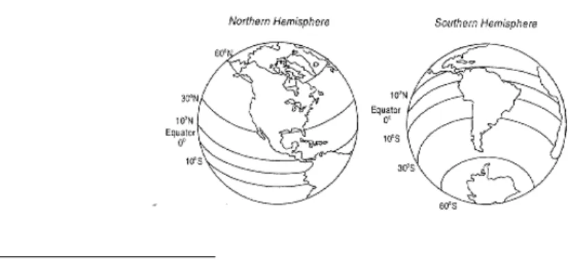
For comparison, we deemed relevant the use of a second series of anomalies, prepared by J. K. Angell31. He constructed it from the average temperatures between 1958 and 1977 with
data from 54 meteorological stations located between the coordinates 10º South and 30º
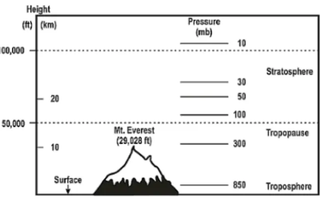
South, the region called subtropical by the author, as illustrated in Figure 2 also varying with altitude, as per Figure 3.
Figure 2. Subtropical region between 10° South and 30° South. Source : JK Angell at
http://cdiac.ornl.gov/trends/temp/angell/angell.html.
27http://data.giss.nasa.gov/gistemp/
28The World Meteorological Organization (WMO) has defined normal weather for the period of 1961 to 1990.
For more details see: WMO, 1996: Climatological Normals (CLIN) for the period of 1961-1990. World Doc Meteorological Organization WMO / OMM No. 847, Geneva, Switzerland, 768 pp.
29http://www.cru.uea.ac.uk/cru/data/landstations/
30The concept of scale adopted here is defined by Gibson et al. (2000). For an example of the application of the
concept to the study of climatic effects on a national scale in Norway - see O'Brien et al. (2004).
*
Figure 3. Altitudes for which temperature anomalies were calculated. The limits of the troposphere, tropopause and stratosphere are indicated. Source: JK Angell in
http://cdiac.ornl.gov/trends/temp/angell/angell.html.
According to Christy et al. (2000) there is a low correlation between surface temperature anomalies and those at other altitudes in tropical and subtropical oceanic regions. However, comparing Angell’s data, we observed positive values between 0.4 and 0.5 for the significant correlations, for both the series that considered the average temperatures for higher pressures or lower altitudes, as well as taking into account the information up to 100 mb (Millibars). The intermediate altitudes series did not provide significant correlations.
Table 1. Correlation between the quantity of anomalies in the subtropical region and other altitudes. Quarterly frequency.
Subtrop. Anom. Up to100 mb 850-300 mb 300-100 mb 100-50 mb 100-30 mb
Correlation 0,478149 0,403089 0,021864 -0,156311 -0,146452
t-Statistic 3,611242 2,921659 0,145067 -1,049750 -0,982044
Probability 0,0008 0,0055 0,8853 0,2996 0,3314
Thus, we deemed that it would be indifferent to use the series for the surface or surface data in combination with altitudes up to 100 mb and we chose the first ones. We did not use the series developed for the 300-850 mb range, even in presence of significant correlation. Other altitude series were not considered because they have no significant correlation with the surface data.
The third series, developed by the Goddard Institute for Space Studies (GISS/NASA) is also monthly. We calculated the quarterly average as in the Jones series, but we also used the monthly data. The anomalies in this case are calculated using 1951-1980 as the reference period32.
The fourth series, extracted from the series of anomalies provided by the GISS was prepared from the average of anomalies at 9-35 degrees south latitude, covering the latitudes over the Brazilian territory. The extraction was performed using FORTRAN programs provided by the
32GISS Surface Temperature Analysis (GISTEMP) available at: http://data.giss.nasa.gov/gistemp/tabledata/SH.Ts+dSST.txt
GISS on its website33. The generation did not include information about temperature
variations in the ocean.
The subtropical temperature anomaly series ended up closer to a normal distribution for the anomaly in the Southern Hemisphere, despite a moderate asymmetry, as per descriptive statistics.
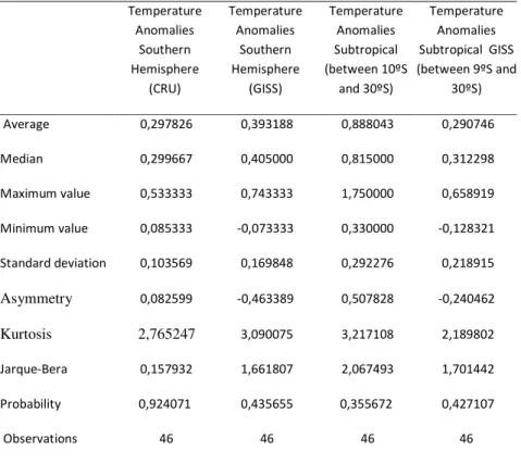
Table 3. Descriptive statistics for the series of temperature anomalies. The anomalies in the southern hemisphere are compared to average temperatures between 1961 and 1990 while the subtropical anomalies are averaged between 1958
and 1977. The subtropical anomaly series of the GISS were calculated over the averages of 1961 and 1990. The frequency is quarterly, between September 1996
and December 2007. All values in degrees Celsius (ºC).
Temperature Anomalies Southern Hemisphere (CRU) Temperature Anomalies Southern Hemisphere (GISS) Temperature Anomalies Subtropical (between 10ºS and 30ºS) Temperature Anomalies Subtropical GISS (between 9ºS and 30ºS) Average 0,297826 0,393188 0,888043 0,290746 Median 0,299667 0,405000 0,815000 0,312298 Maximum value 0,533333 0,743333 1,750000 0,658919 Minimum value 0,085333 -0,073333 0,330000 -0,128321 Standard deviation 0,103569 0,169848 0,292276 0,218915 Asymmetry 0,082599 -0,463389 0,507828 -0,240462 Kurtosis 2,765247 3,090075 3,217108 2,189802 Jarque-Bera 0,157932 1,661807 2,067493 1,701442 Probability 0,924071 0,435655 0,355672 0,427107 Observations 46 46 46 46
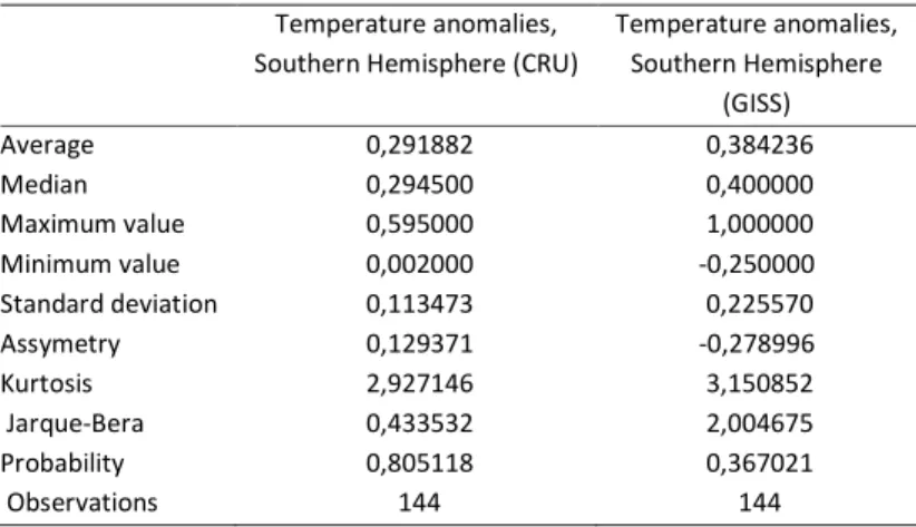
There was an average 0.30 ºC change in temperature between September 1996 and December 2007, according to the Jones series, for the southern hemisphere, or 0.39 °C if we consider the GISS series. The standard deviation of the GISS series is higher than that of the Jones series. If we take the original monthly series of Jones and GISS, according to Table 4, we
33 I thank Professor Reto Ruedy of GISS / NASA for help in extracting and comments on the relationship
between changes in global temperatures and locations. The extraction of the data was made using the program "mkTsMap.f" compiled for win32 platform with GNU gfortran. The input parameters for this program were, for example: "1 1003 2007 2007 1961 1990 9999. 180 90 0 2..." Observe that the second, third and fourth parameter (underlined) were replaced quarter to quarter from 1996 to 2007. Thus, we obtained 46 files from which we could only extract the values of abnormalities for the latitudes -9 to -35, i.e. 9-35 degrees south. Before extracting, the data must be converted to "littleendian" through the "swap.f" program as explained at: https://data.giss.nasa.gov/pub/gistemp/README.txt
observe improvement in the normality index provided by the Jarque-Bera test without major changes in other parameters.
Table 4. Descriptive statistics for the series of temperature anomalies with monthly frequency.
Temperature anomalies, Southern Hemisphere (CRU)
Temperature anomalies, Southern Hemisphere (GISS) Average 0,291882 0,384236 Median 0,294500 0,400000 Maximum value 0,595000 1,000000 Minimum value 0,002000 -0,250000 Standard deviation 0,113473 0,225570 Assymetry 0,129371 -0,278996 Kurtosis 2,927146 3,150852 Jarque-Bera 0,433532 2,004675 Probability 0,805118 0,367021 Observations 144 144
The range of latitudes in the Angell series comprises 90% of the Brazilian GDP, considering the GDP data from municipalities, according to Table 27 (Appendix). The Brazilian population is predominantly urban and concentrated in the south and the southeast regions. According to Figure 14 (Appendices), the latitude range of this GDP percentage is between 12 º South (Salvador) and 30 º South (Porto Alegre). The effect of anomalies is not necessarily felt only over this range, because there is moisture and heat movement between these five Brazilian regions. Over the past five years, the composition of the GDP of the municipalities has not changed much. São Paulo, Brazil's largest city is located at 23.33° South and 46.38º West. IPEA’s Communiqué No. 60 discusses the presence of concentration of municipalities that participate in the GDP:
"The Brazilian pattern of economic growth stands out for recording distinct movements in terms of integrating the municipalities to the development of the Gross Domestic Product since 1920. Currently, few municipalities in the country account for most of GDP, whereas in the past there was less concentration/geographical inequality." (IPEA, 2010 p. 17)
The frequency of Angell´s series follows the seasons, starting in the Northern Hemisphere winter (December, January and February). We assume that the effects of temperature do not occur immediately, therefore the lag of a month in the seasonal quarter of Angell's series compared to the economic quarters didn’t seem to be an obstacle to using this series.34
Bansal and Ochoa (2010) analyzed the temperature effect in the capital markets and concluded that the countries close to the equator, and therefore close to the latitude range of the series of subtropical anomalies, have a positive risk premium related to temperature that decreases with distance from the equator.
34Here's a suggestion for further evaluation: Is there much difference in the results obtained if the Economic
It is worth noting that the temperature anomalies in the southern hemisphere don´t have the same historical behavior as the anomalies of the northern hemisphere, due, according to Jones (2003), to a larger ocean area:
" The SH" (...) " in contrast shows less seasonal contrasts in both trends and year-to-year variability than the NH, a result that might be expected given its greater ocean fraction. Warming is statistically significant for all seasons and annually for 1861–2000, 1901–2000, all seasons except summer (DJF) for 1920–44, and all seasons except summer and autumn (MAM) for 1977–2001. There is no evidence of cooling during the 1945–76 period. For all periods the winter (JJA) always warms by the greatest magnitude." (p. 217)
Comparative graphs of the temperatures series are shown in Figure 13 (Appendices). Unit root tests of the subtropical anomalies series demonstrated them to be non-stationary at a significance level of 1%, according to Table 21 (Appendix). All other anomalies series are stationary at usual levels of significance.
As there was indication of lack of normality in some univariate series, we decided to assess whether the classical Spearman correlation would be the most apt to evaluate the relationships between the temperature series. Mundfrom and Mecklin (2004) cite the work of Bilodeau & Brenner (1999) to present the case of two variables that are distributed usually univariately, but, together, are not normal, as they have a Frank density function35 as per Figure 4.
Figure 4. Extracted from Bilodeau & Brenner (1999), p. 27. Frank bivariate density with normal marginal distribution pattern and a correlation of 0.7.
One of the possible tests to assess the deviation from normality is through the Shapiro-Wilk W statistics36, a kind of multiple correlation. The closer W is to one, the smaller the deviation
from normality. The statistics do not allow asserting the existence of a normal bivariate, but is indicative of deviation.
35 For more details, see Genest, C. (1987). Frank's family of bivariate distributions. Biometrika 74, 549-555. 36The W statistics of Shapiro-Wilk test was implemented in the statistical package "R" available at:
https://cran.r-project.org/web/packages/mvnormtest/index.html . MECKLIN and MUNDFROM (2004) discuss advantages and disadvantages of other tests of multivariate normality.
Table 5. Bivariate normality tests between combinations of temperature anomalies series.
Joint Normality Test W Statistic P-value
Jones Series / GISS Series 0.9536 0.0649
Jones Series / Angell Series
0.9662 0.1993
GISS Series/ Angell Series 0.9772 0.4945
The p-values found led us to decide to use the Spearman rank method, instead of the classical method, as noted by Neter (1996, Chapter 15 - Normal Correlation Models p. 651).
Table 6. By Spearman rank correlation. The p-values were adjusted by Bonferroni method to allow for multiple comparisons37
Correlation t-Statistic
Probability Jones Series GISS Series Angell Series GISS Subtropical series
Jones Series 1.000000 --- --- GISS Series 0.451164 1.000000 3.353370 --- 0.0099 --- Angell Series 0.409972 0.228239 1.000000 2.981526 1.555011 --- 0.0280 0.7626 ---
GISS Subtropical series 0.712387 0.580028 0.376516 1.000000
6.733443 4.723165 2.695914 ---
0.0000 0.0001 0.0594 ---
The linear correlation between the series is positive, but when the GISS and Angell series were combined there was no significance. As the 0.45, 0.40 and 0.71 correlation values between Jones and GISS, Jones and Angell, and Jones and subtropical GISS, respectively, are significant, we could only use the GISS and Angell series, but the descriptive statistics of Table 3 led us to believe that the series are different enough. Even the correlation between the southern hemisphere GISS series and the subtropical latitudes is not so high as we initially expected, although significant with a value of around 0.58.
If we lag the GISS or subtropical GISS series in one period, and do the lagged correlation with the Angell series, we find a positive and significant relationship.
37For more details on multiple tests of hypotheses, see Shaffer, Juliet Popper (1995). Multiple
Table 7. By Spearman rank correlation with lags. The same criterion of the previous table, but lagging the GISS and subtropical GISS series in a quarter. The gap can also be observed in Figure 13 (Appendix).
Correlation t-Statistic Probability
GISS series lagged a quarter Angell Series GISS subtropical series lagged a quarter
GISS series lagged a quarter 1,000000 --- --- Angell Series 0,490738 1,000000 3,693287 --- 0,0019 ---
GISS subtropical series lagged a quarter 0,573462 4,590198 0,0001 0,411020 2,956520 0,0151 1,000000 --- ---
3.1.4 Claims
We used direct claims data from Statistics System of Private Insurance Superintendency (SES / SUSEP)38. Direct premiums, net written premiums, claims and direct retained claims are
among the information that can be obtained from the SES. We extracted the claims series directly with monthly frequency, for each line of business, available since 1995.
The information is reported in accordance with accrual accounting in order to reflect the balance of the obligations of insurers and reinsurers as soon as their existence is known. We chose to disregard the effect of the variation in technical provisions for claims (claims that are incurred but not reported, and their variations and outstanding claims), upon understanding that there are more relevant factors that interfere with the oscillation of these reserves than those linked to climate changes and that, therefore, in relative terms, the effect of temperature anomalies in the variation of the reserves is small.
Due to changes in the way that businesses are broken into smaller parts called branches, and aggregated in “groups” starting with SUSEP Circular No. 295/200539, it was necessary to
combine the grouping of information from an old code together with the new ones. In some cases, extinct branches, like Branch 11 (Fire), are not cited because the claims information was added to the branch or the branches that succeeded it (e.g. Branch 96 - Specified and Operational Risk).
Through these procedures, we obtained the first series of nominal claims, built by the claims aggregation of all branches. As the consumption series were deflated by the INPC (National Consumer Price Index), we used this index for the real claims series "A". It may be worth analyzing the model behavior with more than one price index, because SUSEP Circular No. 255/200440 allowed the insured and insurers to agree for indices in order to "update
operational figures related to insurance, open private pension and capitalization." The studies on the effect of other indices should take into consideration their correlation with the
38http://www2.susep.gov.br/menuestatistica/SES/principal.aspx
39http://www2.susep.gov.br/bibliotecaweb/docOriginal.aspx?tipo=1&codigo=18782 40 http://www.susep.gov.br/setores-susep/seger/coate/orientacoes-ao-consumidor-pgbl-vgbl/circ255%20e%20anexos.pdf/view?searchterm=SEGURADORA
INPC. We observed that the IPCA (Extended National CPI), for example, has a correlation of 0.96 with the INPC for the sample studied, so it's not a good candidate for further analysis. We do not delve into the discussion of the best discount rate for the claims series, understanding that the price indices chosen here reflect the changes in a basket of prices that applies to the economy as a whole, including therein the series of aggregate claims. Some considerations on the concept of present value applied to the insurance market and reinsurer can be found in the work of the IAIS (International Association of Insurance Supervisors) (2003, p. 11 and 12).
After aggregating the data, we observed the existence of outliers, as illustrated in Figure 11 (Appendix). Given its nature as an unexpected event in time of undetermined severity, we took as a reference the definition of what would be an outlier, the P-36 accident in 2001. In the time series of Marine Hull claims (branch 0234), which contained the above occurrence, we noted that four standard deviations above the mean of the series would be sufficient to identify these cases. Thus, besides the Hull branch, we identified three further points out of trend for the series: two in the field of Aviation in 2006 and Hulls 2007 (GOL and TAM accidents) and one related to Specified/Operational risks in 2005 (CSN)41. The causes of such
claims are not related to variations in temperature, which strengthened the justification for the exclusion of these values from the series. Figure 12 (Appendix) makes a comparison between the “B” claims series, after the removal of outliers, with the "A" series42.
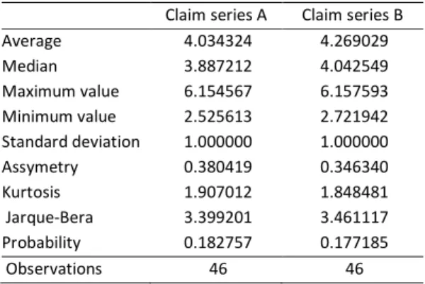
Thus, the two series obtained, "A" and "B", were normalized dividing them by their corresponding standard deviations. Doing so, we reduced the problem regarding differences in order magnitude between the consumption series and the series of claims that affected the coefficients estimated by the model, notwithstanding their significance.
Table 8. Descriptive statistics of the series of direct losses normalized by dividing the original series by the standard deviation of the series. “A” series claims include outliers.
Claim series A Claim series B
Average 4.034324 4.269029 Median 3.887212 4.042549 Maximum value 6.154567 6.157593 Minimum value 2.525613 2.721942 Standard deviation 1.000000 1.000000 Assymetry 0.380419 0.346340 Kurtosis 1.907012 1.848481 Jarque-Bera 3.399201 3.461117 Probability 0.182757 0.177185 Observations 46 46
41The names of the insured were mentioned because all these accidents are of public knowledge and gained
wide dissemination in the press (GOL: http://pt.wikipedia.org/wiki/Voo_Gol_Transportes_Aéreos_1907,
TAM: http://pt.wikipedia.org/wiki/Voo_TAM_3054 and CSN: https://oglobo.globo.com/economia/explosao-interrompe-producao-de-alto-forno-da-csn-4602245)
42We intend to conduct event studies to determine the effect of these large claims on the stock price of their
companies on the BOVESPA. All the three major insured parties were listed on the Brazilian stock exchange upon the occurrence of the respective claims.
We also observed the lack of stationarity in the claims series, using usual levels of significance, according to Table 22 (Appendix), which led us to use growth rates of loss models instead of the levels of claims.
Table 9. Descriptive statistics of claims rate series.
Claims rates A43 Claims rates B
Average 0,007388 0,007388 Median 0,009440 0,009440 Maximum value 0,139664 0,050763 Minimum value -0,140191 -0,031072 Standard deviation 0,037417 0,019934 Assymetry -0,437714 0,095540 Kurtosis 9,659345 2,475441 Jarque-Bera 84,58734 0,584387 Probability 0,000000 0,746624 Observations 45 45
We have observed, as described by the IAIS (2006), that the claim information can be biased and not be a good estimator of losses, but we keep in line with the thought that:
"Just as premiums can be biased by various factors which do not relate directly to the risks assumed (e.g. the market), claims may not be an accurate predictor of future losses. They may, however, be useful proxies for the risk being assumed." "(p. 40)
3.2 Methods
3.2.1 Study of the Correlations
Our first hypothesis is that there is positive and significant correlation between temperature anomalies and direct claims. To observe the effect of the three series of anomalies on the claims series, we try to evaluate, initially, how they are correlated with each class of insurance, in particular.
Before performing the correlations, as was done with the temperature anomalies series, we performed Shapiro’s bivariate normality test, and noticed that we should not consider the existence of normal bivariate distribution branch to branch, as in Table 19 (Appendix). In this case, however, no significance was found in the correlations, according to Table 20 (Appendix).
43The series of charges corresponding to log (incident / accident (-1)) / log (10)). We could not find in literature
a detailed description of procedures used to calculate the rate of growth. We evaluated some alternatives and noted that, in general, using log base 10 got a value closer to the reported. The magnitude of rates is less important than their variation for the purposes of this study.
Table 10. Correlations by Spearman rank method with multiple comparisons adjusted by Bonferroni between the real claims series A and B, with outliers, and the temperature anomalies series, contemporaneous and lagged one period (-1). The series
frequency is quarterly.
Claims series Temperatura Anomaly Series Correlation t-Statistic Probability
A Jones -0,016590 -0,110061 1,0000 GISS 0,249615 1,709881 0,5660 Angell 0,370654 2,647196 0,0673 Subtrop GISS 0,155350 1,043139 1,0000 A Jones (-1) 0,099279 0,654246 1,0000 GISS (-1) 0,319080 2,207753 0,1959 Angell (-1) 0,392117 2,795129 0,0463 Subtrop GISS (-1) 0,258762 1,756642 0,8610 B Jones 0,005797 0,038455 1,0000 GISS 0,296552 2,059759 0,2722 Angell 0,337581 2,378907 0,1306 Subtrop GISS 0,212088 1,439579 1,0000 B Jones (-1) 0,085247 0,561041 1,0000 GISS (-1) 0,297206 2,041146 0,2844 Angell (-1) 0,384735 2,733260 0,0544 Subtrop GISS (-1) 0,239921 1,620601 1,0000
Despite being encouraged by the improvement in correlation between the claims series and the anomalies series lagged one period, the justification may be the elimination of one of the observations due to the displacement of the anomalies series. If we continue with more lagged periods, the correlation tends to increase and becomes more likely to indicate significance. As we have no residuals in this analysis, we cannot evaluate the effect of other factors on the correlation. The claims series with outliers has a higher significant correlation in comparative terms.
Table 11. Correlations by the Spearman rank method with Bonferroni-adjusted multiple comparisons between the real claims series A and B, with outliers, and the GISS and Jones temperature anomalies series, contemporaneous and lagged one period (-1). The series frequency is monthly.
Claim series Anomaly series Correlation t-Statistic Probability
A Jones 0,135137 1,625248 0,3190 GISS 0,284520 3,536609 0,0016 B Jones 0,140651 1,692876 0,2780 GISS 0,301928 3,774015 0,0007 A Jones (-1) 0,179101 2,161661 0,0970 GISS (-1) 0,302109 3,763192 0,0007
B Jones (-1) 0,174605 2,105669 0,1110 GISS (-1) 0,303710 3,785154 0,0007
In the case of the Jones and GISS series, we also have available for analysis a monthly frequency, and, according to Table 11, the GISS series becomes correlated positively and significantly with the claims series with or without outliers.
For the quarterly frequency, the scale of subtropical series at a significance level of 10% can be considered positively correlated with the real claims series, whether considering the major claims as outliers, or not. The same is not true with the GISS subtropical series. The other series were not correlated at the usual levels.
The GISS monthly series is also positive and significantly correlated with the claims series.
3.2.2 Pricing
Knowing that correlations between temperatures and claims exist, we moved on to the second stage in which we seek to verify whether we can build a pricing model conditional on the claims series or temperatures anomalies that would generate better results than those reported in the literature with the classical CCAPM model.
Even knowing the limitations of the CCAPM in terms of not explaining the EPP (Equity Premium Puzzle), and using standard utility functions that do not detach the risk aversion coefficient from intertemporal consumption elasticities, among others, based on the results of Cysne, Issler and Piqueira, we believe that an initial approach with a more simple model would be more substantive.
The CCAPM is bad if tested unconditionally, but in our model we use, for example, the temperature and claims series as instrumental variables. We will check to verify whether the model’s explanatory power improves.
In line with the method proposed by Fama and Macbeth (1973), the model is estimated in two stages, the first one consisting of using asset portfolios to obtain estimates of beta coefficients to be used in the second stage. That is, the first step is the implementation in time series for the entire period:
?@, = A + A * , , with j = 1 .. n (1)
Where *, is any factor44 that varies in period "t" with the ability to explain the portfolio
returns. This may include n factors to estimate their betas.
For our data, "i" ranges between 1-6 for the criteria used in the preparation of portfolios, and for each of the five categories, totaling 30 portfolios, while "t" for each portfolio, covers the 46 quarters from September 2006 to December 2007. We then obtain 30 estimates of A , and
44 Usually the factors are not asset portfolios. If you want to work that way see Shanken (1992) for