Braz. j. oceanogr. vol.56 número3

LOBSTER (Panulirus argus) CAPTURES AND THEIR RELATION

WITH ENVIRONMENTAL VARIABLES OBTAINED BY ORBITAL SENSORS FOR

CUBAN WATERS (1997-2005)

Regla Duthit Somoza1, Milton Kampel2, Frederico de Moraes Rudorff 2, Ronald B. Sousa2 and Susana Cobas3

Instituto Nacional de Pesquisas Espaciais – INPE 1_{Centro de Previsão de Tempo e Estudos Climáticos –CPTEC}

2

Divisão de Sensoriamento Remoto

(Avenida dos Astronautas, 1758, Jd. Granja, 12227-010 São José dos Campos, SP, Brasil) regla.somoza@cptec.inpe.br, milton@dsr.inpe.br, ronald@dsr.inpe.br, fmr@dsr.inpe.br,

3

Centro de Investigaciones Pesqueras

(5ta _{Ave.y 246, Barlovento, Sta. Fe, Playa, Ciudad Habana, Cuba. CP: 19100, Cuba)} susana@cip.telemar.cu

A

Chlorophyll concentrations (Chl a) data obtained from the Sea Viewing Wide Field of View Sensor (SeaWIFS) ocean color monthly images, Sea Surface Temperature (SST) pathfinder data obtained from the Advanced Very High Resolution Radiometer (AVHRR) sensors, and lobster (Panulirus argus) captures at the Cuban shelf were examined in order to analyze their spatial and temporal variability. A cross-correlation analysis was made between the standardized anomalies of the environmental variables (Chl a and SST) and the standardized anomalies of lobster captures for each fishery zones for the period between 1997 and 2005. For the deep waters adjacent to the fishing zones it was not observed a clear Chl a seasonality and on average the lowest values occurred south of the Island. It is with the three years lag that Chl a had the greatest numbers of significant correlation coefficients for almost all fishing zones. However, the cross-correlation coefficients with SST showed higher values with 1,5 year lag at all zones. Since the two environmental variables obtained by satellite sensors (SST and Chl a) influence the lobsters mainly during the planktonic life cycle, the cross-correlation with lobster captures begin to show significant indexes with lags of 1.5 years or more.

R

Dados de captura da lagosta Panulirus argus na plataforma cubana foram comparados com concentrações de clorofila (Chl a) e valores de Temperatura de Superfície do Mar (TSM) obtidos pelos sensores Sea Viewing Wide Field of view Sensor (SeaWIFS) e Advanced Very High Resolution Radiometer (AVHRR), respectivamente. Uma análise de correlação cruzada foi realizada entre as anomalias padronizadas das variáveis ambientais (Chl a e TSM) e as anomalias padronizadas de capturas da lagosta para cada zona de pesca no período 1997-2005. Para as águas profundas adjacentes às zonas de pesca não foi observada uma sazonalidade evidente da Chl a. De forma geral, os menores valores de Chl a ocorreram ao sul da Ilha. Na maioria das zonas de pesca, a captura da lagosta apresentou os maiores coeficientes de correlação com valores de Chl a com defasagem de dois e três anos. Já em relação à análise com dados de TSM, os coeficientes de correlação cruzada apresentaram valores significativos apenas a partir de uma defasagem de 1,5 anos para praticamente todas as zonas de pesca. Neste estudo confirma-se que, em águas cubanas, correlações cruzadas significativas entre estas duas variáveis ambientais medidas por satélite e as capturas da lagosta espinhosa ocorrem principalmente durante o ciclo de vida planctônico desta espécie.

Descriptors:Chlorophyll a, Sea surface temperature, Lobster captures, Cross-correlation.

Descritores: Concentração de clorofila, Temperatura de superfície do mar, Capturas da lagosta, Correlação cruzada.

I

The Caribbean spiny lobster, Panulirus argus is widely distributed throughout the tropical and

are usually recorded at shallow waters, but they may occur on depths up to about 90 m (TAVARES 2002; LEÓN et al., 2005). This lobster is one of the most economically important species in the Caribbean. About 26 countries are involved in the fishery and the commercialization. Cuba, the Bahamas and Brazil, are the largest producers with more than 60% of the total catch in the region, followed by United States, Honduras and Nicaragua (EHRHARDT, 2001).

In Cuba the spiny lobster is the most important marine resource. The fishery profits are around US$ 80 million per year and there are thousands of people on coastal communities dedicated to extractive and industrial activities related to lobster fishery (BAISRE, 2000). However, the captures have been decreasing from an average of 11000 ton in the 80's to an average of 6500 ton in 2005, representing a reduction of 36%, besides the great interannual variability of captures that exists (PUGA, 2005). These facts are leading the scientific community to study biotic and environmental variables that can explain the diminution in captures, as well as to contribute to future fishing operation forecasting.

The lobster is a crustacean that has both benthic and planktonic stages during its life cycle. The adult female, which is benthic , after mating they incubate their eggs and release them at the edge of the shelf, which mainly happens between February and May (CRUZ; LEÓN 1991). The phyllosomata larvae are oceanic and planktonic, and concentrate in the water column between 0 and 50 m depths (AUSTIN, 1972; YEUNG; MCGOWAN, 1991; YEUNG; LEE 2002). After metamorphose into post-larvae, a stage that begins to resemble the adult, they can swim actively near the surface towards the coast (CALINSKY; LYONS, 1983). This takes place every month of the year, but there is a main peak between September and December (CRUZ et al. 1995).

When they arrive at the coast they settle in clumps of algae or any other structure suitable for hiding and mute again into juveniles (CRUZ et al,.

1995). Around July and August, usually 10 to 15 months after settlement, the juveniles go to the nursery grounds where they live hidden in caves, coral reefs and sponges, amongst others. Later on, between March and May, the juveniles enter the fishery ground. This happens approximately two and a half years after the eggs have hatched (LEÓN et al., 1991; CRUZ et al., 1991).

The lobster fishing resource forecasting and estimation must be studied by measuring the parameters that affect its distribution and abundance. For many years, environmental variables have been used to correlate the spatial and temporary distribution of marine species (SANTOS, 2000).

For the Batabanó Gulf, Baisre and Cruz (1994) suggested that the strong winds of Hurricane

Gilbert affected the marine floor of the spiny lobster nursery grounds through the southern coast of Cuba, in 1988. Alfonso et al. (1999) outline the gradients of SST and depth as being the two main factors that influence the larval dynamic. Moreover, they indicate a limitation of the panulirus larval distribution on the water column related to the thermocline and the restriction of larval movement over the 26°C isotherm for Cuban waters.

Baisre et al. (1984), Hernández (1988), García et al. (1991), Hernández et al. (1995), Hernandez and Puga (1995), studied the massive lobster migrations that occur in the period between October and December. They related this behavior as a response to the first strong environmental perturbation such as cold fronts and tropical hurricanes. Also, Hernandez (2002) studied the influence of sea surface temperature (SST) anomalies on spawns and recruitments of the spiny lobster Panulirus argus at the Batabanó Gulf, all with good levels of statistical significances considering the lags between recruitment and the adult phase suitable for fishery. Somoza et al.

(2006) analyzed the cross-correlation between SST anomalies derived from the Advanced Very High Resolution Radiometer (AVHRR) sensors and lobster captures between 1997 and 2004.

In spite of the good results obtained in scientific researches where satellite information are used to help fishing activities, there are few institutions of this economic branch that recognize and/or apply this potential to develop the fishing sector (SOUZA, 2005). Most of the remote sensing applications that are used on fishing activities have as a primary target to increase fishery productivity. According to Santos (2000), some advantages of the uses of remote sensing techniques in the aid of fishery activities are: a) fuel economy when searching certain species; b) smaller costs with the crew; and c) reduction of maintenance costs with boats.

The ocean color measurements intrinsically include chlorophyll concentration (photosynthetic pigments of the phytoplankton), which is commonly considered as a biological productivity index for oceanic environment (GOWER, 1972).

In this context, this work has as main objective to analyze the relations between environmental variables (chlorophyll concentration and Sea Surface Temperature) and lobster captures at the deep water adjacent to Cuban Shelf fishing zones, for a time series from 1997 to 2005. It also aims to improve the analysis of Somoza et al. (2006), who compared SST data and lobster captures, by making a reanalysis with the anomalies of both variables for the same period.

M

M

Study Area

The selection of the study area was determined by taking into account the spatial distribution of the spiny lobster life cycle over the Cuban waters. According to Cruz et al. (1990) and a consideration of FAO (2003), the Caribbean lobster population could be interconnected through the water circulation regimen. Therefore, the area selected is located between 18°-25°N and 73°- 87°W.

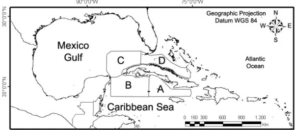
The study area was divided into regions of interest (ROI) which are oceanic waters adjacent to the Cuban spiny lobster fishery zones (Fig. 1) described below:

• “Jardines de la Reina” Archipelago (Zone A), situated in the southeast shelf of Cuba (18328,8 km2). This region includes 661 keys and islets, and

the southeastern shelf of Cuba defined by the Gulf of “Ana María” and the Gulf of “Guacanayabo”;

• “Los Canarreos” Archipelago (Zone B), situated in the southwestern shelf of Cuba (21851.2 km²). This region includes 672 islands, keys, and islets, the biggest of which is “Isla de la Juventud” and the southwestern shelf of Cuba defined by the Gulf of “Batabanó”;

• “Los Colorados” Archipelago (Zone C), situated in the northwest shelf of Cuba (3432.5 km²); with 160 keys and islets; includes the northwestern shelf of Cuba defined by the Gulf of “Guanahacabibes”;

• “Sabana-Camagüey” Archipelago (Zone D), situated in the northeastern shelf of Cuba (10739.8 km²), is also known as “Jardines del Rey”. This region consists of 2,517 islands, keys and islets; it includes the northeastern shelf of Cuba and several large bays.

In the insular shelf waters, the bathymetry is characteristic of shallow waters. They have a mean depth of about 7 m at the occidental and north-oriental regions (Zones B, C, and D), and greater depths for the southern oriental region, oscillating between 15 and 25 m (Zone A). At zones where the coastline is not surrounded by shallow waters, depths strongly increase a few km away from the coast. The bathymetry of the ROIs are typical of deep waters, oscillating between 500 to 5500 m, thus being classified as Case I waters (MOREL, 1980; MOREL; PRIEUR, 1977).

Data Set

The fisheries zones were obtained from the Biologic-Fisher Lobster Atlas (CRUZ et al., 1990). Monthly catches in metric tons for the whole period (1997-2005) were taken from statistical books from the Ministry of Fishery Industry to every fishery zone. The standardized anomalies were then calculated for each fishing zone.

The chlorophyll pigments have a specific and distinguishing spectral signature. They absorb in wavelengths corresponding to blue (455-492 nm) and red (622-700 nm) colors and they have strong reflectance in green (492 – 577 nm). On deep waters away from the coast lines, known as Case I waters (MOREL; PRIEUR, 1977; MOREL, 1980), the ocean color is mainly modified by photosynthetic organisms (STEWART, 1985). Thus, Chl a values can be quantified by orbital ocean color sensors.

The Chl a data were obtained from SeaWIFS images that are available on the Ocean Color web site at <http://oceancolor.gsfc.nasa.gov/cgi/level3.pl.> The Level 3 data are available HDF format on a global scale with cylindrical equidistance projection. They have a spatial resolution of 9x9 km and are monthly binned. There are 100 images for the period between September, 1997 and December, 2005. All images were previously corrected for atmospherically effects (GORDON; WANG, 1994).

The SST data used was the AVHRR Oceans Pathfinder Global 4 km equal-angle all SST v5 (NOAA, NASA) product for the period between 1997 and 2004, which was the same used by Somoza et al.

(2006). In order to complete the series, monthly mean SST data of each ROI were obtained from analysis of 9x9 km spatial resolution MODIS Aqua monthly SMI (Standard Mapped Image) products from the Ocean Biology Processing Group (OBPG), available online:< http://reason.gsfc.nasa.gov/OPS/Giovanni/ocean.aqua. shtml>.

Image Processing

SeaWiFs data were processed with the routines Swl10 (version 3.0) and SeaDAS ® software, both distributed by the SeaWiFS Project (NASA), using respective standard algorithms and masks. Chlorophyll a values were obtained using a global algorithm (O'REILLY et al., 2000). Each image was cut using the respective Region of Interests (ROI) boundaries. The monthly mean, climatology and standardized anomalies (mean=0 and standard deviation=1) values of Chl a were calculated for each ROI using IDL scripts to the ENVI® software (ITT Visual Information Solutions).

Correlation Analyses

Taking into account that some authors (HERNÁNDEZ, 2002; SOMOZA, 2006) studied the influence of sea surface temperature (SST) anomalies on spawns and recruitments of the spiny lobster

Panulirus argus observing good levels of statistical significances considering 2 years of lagging between recruitment and the adult phase suitable for fishery; and also that Ciotti and Kampel (2001) observed that there is a clear relationship between the decrease in temperature and the increase in chlorophyll a

concentration, a cross-correlation analysis was made between the standardized anomalies of the environmental variables (Chl a and SST) and the standardized anomalies of lobster captures for each ROI. Since the correlations are not made directly between larvae data and environmental variables, but between captures of adult lobsters, the correlations were made taking into account time lags of 1.5, 2 and 3 years. Correlation analysis for the closed season months will not be shown on the graphics and tables of this work due to the fact that there are no captures allowed during this period.

R

Chl a climatology and Anomalies

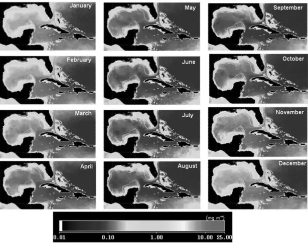
Chlorophyll concentration (Chl a) climatology images (Fig. 2) of the study area showed larger concentrations and stronger variations at the Gulf of Mexico than at the Western Caribbean Seas. The concentrations were also the highest around the coastal zones, especially at the mouth of the Mississippi River in the Gulf of Mexico.

A seasonal behavior is also evident along the year. In spring and summer (from April to September), the values were generally lower. At areas of water deeper than 500 m, the values were lower than 0,10 mg/m3 and for shallow coastal waters the Chl a varied between 0.25 and 1 mg/m3. In fall and winter (from October to March) the Chl a had a slight increase with values exceeding 0.10 mg/m3 at deep waters and 2 mg/m3 at shallow waters.

Fig. 2. Climatologic SeaWiFS images (Sep/1997-Dec/2005 period). In white a 500 m depth line.

0,1 0,15 0,2 0,25 0,3 0,35 0,4

Ja

n

Feb Mar Ap

r

M

ay

Ju

n

Ju

l

Au

g

Se

p

Oc

t

No

v

De

c

Ch

l-a

(

m

g

/m3

)

Zone A Zone B Zone C Zone D

The Chl a time series vary on a similar way for all 4 zones with high cross-correlation coefficients between them (Table 1). The zones south of the Island (A and B) present the highest correlation (0.87) while for the northern zones the correlation coefficient is lower, but significant (0.68). As it was expected, due to the greater distance, the lowest correlation coefficients were found amongst zone D and the southern zones A and B (0.37 and 0.20, respectively).

Table 1. Cross-correlation coefficients for each ROI.

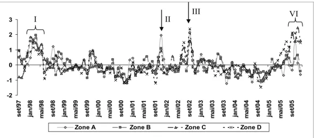
The amplitude variability of the Chl a

anomalies (Fig. 4) reach 0,11 mg/m3 on average. The positive maximums that stand out occurred in the following periods: I) Jan-Mar/1998; II) Nov/2001; III) Sep/2002 y IV) Jul-Nov/2005. Zone A presented a maximum positive anomaly in Nov./2001 (0.04 mg/m3) and a minimum in Oct./2003 (-0.02 mg/m3). The Zone B reached a maximum in Mar/1988 (0.04 mg/m3) and a minimum in Nov/2000 (-0.02 mg/m3). The Zone C showed a maximum in Nov/2005 (0.11

mg/m3) and a minimum in Oct/2000 (-0.05 mg/m3). The Zone D achieved the maximum in Sep./2005 (0.09 mg/m3) and a minimum in Oct/2004 (-0.06 mg/m3_{). Maximum amplitudes were observed on the} north at Zone C (0.16 mg/m3). On the southern side of the Island they were similar for both zones (0.06 mg/m3).

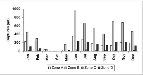
Fisheries

Two periods per year can be described for lobster fishery: one after the closed season, with maximums in June; and another at the end of the year, called recalo. The second period begins when the first strong environmental perturbation such as cold fronts and tropical hurricanes appears, mainly in October, November or December, depending on the area.

The closed season is a protection measure that occurs from March to May, which has been extended recently to 110 days including February or June, indistinctly. The closed season protects both the spawning and the recruitment at the fishing areas, during the peak months for these processes (ARCE; LEÓN 2001). In addition, there is a regulation on the minimal legal length of caught (72 mm of carapace length since 2006). The spiny lobster reaches this minimal legal length with 1.5 years of age, approximately (CRUZ; LEÓN 1991).

-2 -1 0 1 2 3 se t/ 9 7 ja n /9 8 ma i/ 9 8 se t/ 9 8 ja n /9 9 ma i/ 9 9 se t/ 9 9 ja n /0 0 ma i/ 0 0 se t/ 0 0 ja n /0 1 ma i/ 0 1 se t/ 0 1 ja n /0 2 ma i/ 0 2 se t/ 0 2 ja n /0 3 ma i/ 0 3 se t/ 0 3 ja n /0 4 ma i/ 0 4 se t/ 0 4 ja n /0 5 ma i/ 0 5 se t/ 0 5

Zone A Zone B Zone C Zone D

I II

III

VI

Fig. 4. Chl a anomalies Sep/1997- Dec/2005 period (Mean=0 and Standard deviation = 1). Items I, II, III, IV are the higher positive variability for the time series.

Z one A Z one B Z one C Z one D

Zone A 1

Zone B 871 1

Zone C 523 573 1

0 200 400 600 800 1000

Ja

n

Fe

b

Ma

r

Ap

r

Ma

y

Ju

n

Ju

l

Au

g

Se

p

Oc

t

No

v

De

c

C

a

pt

ur

e

s

(

m

t)

Zone A Zone B Zone C Zone D

Fig. 5. Monthly mean for each fishery zone (1997- 2005 period). Note that on the closed season period (March-May), captures are not allowed.

Cross-correlation Coefficients

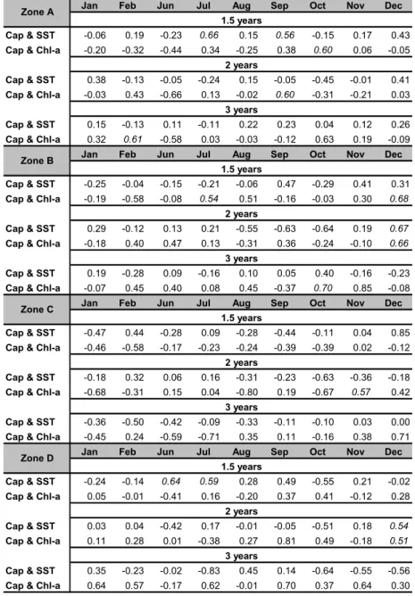
An analyze was made taking into account the annual anomalies mean for each variable (Fig. 6). It was observed that between TSM and Captures, better correlation coefficients correspond to 1.5 years of lagging on the zone A and D (0.3 for both). Between Chl a and captures the correlation coefficients were better for 3 years of lagging (Zone D with 0.4).

In general, cross-correlation coefficients reach highest values between Chl a and captures for annual mean anomalies than for SST and captures. Looking for a detailed analysis on behalf of each study zone a monthly cross-correlation evaluation was made (Table 2).

At Zone A, it was observed for 1.5 year of

lagging the best correlation with SST in July while for Chl a it occurred in October. For 2 years of lagging, correlation coefficient with SST was low, getting the best (-0.45) in October, but to Chl a this coefficient reached up to -0.66 in June. With tree years of lagging, significant correlation values were observed for Chl a

in February, June and October.

For Zone B, it was observed for 1.5 year of lagging the best correlation of captures with SST in September while for Chl a it was in December. For 2 years of lagging the best correlation coefficient found for SST was in December, for Chl a coefficient, it also reached up this maximum in December. With tree years of lagging, significant correlation values were observed for Chl a in October and November and for SST in October.

Fig. 6. Annual mean standardized anomalies cross-correlations (left side: SST and Captures; Right side: Chl a and Captures).

-0,3 -0,2 -0,1 0 0,1 0,2 0,3

0 1.5 2 3

Years of lagging

TS

M

&

C

A

P

co

rr

el

at

io

n

s

-0,2 -0,1 0 0,1 0,2 0,3 0,4

0 1.5 2 3

Years of lagging

C

H

L

-a & CAP

co

rr

e

lat

io

n

s

At zone C, it was determined the best correlation with SST in December while for Chl a it was in February for 1.5 year of lagging. Taking into account, 2 years of lagging the captures best correlation coefficient with SST was in October, and with Chl a in January and October. With tree years of lagging, significant correlation values were observed for Chl a in July and December and for SST in February.

For zone D, the best correlation calculated between captures and SST was in June while for Chl a in June and October for 1.5 year of lagging. Regarding 2 years of lagging the captures best correlation coefficient with SST was in December, and with Chl a also in December.. With tree years of lagging, significant correlation values were observed for Chl a in September and for SST in July.

Table 2. Cross correlation coefficients (Cap & SST and Cap & Chl-a), with 1.5; 2 and 3 years of lagging).

Jan Feb Jun Jul Aug Sep Oct Nov Dec

Cap & SST -0.06 0.19 -0.23 0.66 0.15 0.56 -0.15 0.17 0.43

Cap & Chl-a -0.20 -0.32 -0.44 0.34 -0.25 0.38 0.60 0.06 -0.05

Cap & SST 0.38 -0.13 -0.05 -0.24 0.15 -0.05 -0.45 -0.01 0.41

Cap & Chl-a -0.03 0.43 -0.66 0.13 -0.02 0.60 -0.31 -0.21 0.03

Cap & SST 0.15 -0.13 0.11 -0.11 0.22 0.23 0.04 0.12 0.26

Cap & Chl-a 0.32 0.61 -0.58 0.03 -0.03 -0.12 0.63 0.19 -0.09

Jan Feb Jun Jul Aug Sep Oct Nov Dec

Cap & SST -0.25 -0.04 -0.15 -0.21 -0.06 0.47 -0.29 0.41 0.31

Cap & Chl-a -0.19 -0.58 -0.08 0.54 0.51 -0.16 -0.03 0.30 0.68

Cap & SST 0.29 -0.12 0.13 0.21 -0.55 -0.63 -0.64 0.19 0.67

Cap & Chl-a -0.18 0.40 0.47 0.13 -0.31 0.36 -0.24 -0.10 0.66

Cap & SST 0.19 -0.28 0.09 -0.16 0.10 0.05 0.40 -0.16 -0.23

Cap & Chl-a -0.07 0.45 0.40 0.08 0.45 -0.37 0.70 0.85 -0.08

Jan Feb Jun Jul Aug Sep Oct Nov Dec

Cap & SST -0.47 0.44 -0.28 0.09 -0.28 -0.44 -0.11 0.04 0.85

Cap & Chl-a -0.46 -0.58 -0.17 -0.23 -0.24 -0.39 -0.39 0.02 -0.12

Cap & SST -0.18 0.32 0.06 0.16 -0.31 -0.23 -0.63 -0.36 -0.18

Cap & Chl-a -0.68 -0.31 0.15 0.04 -0.80 0.19 -0.67 0.57 _0.42

Cap & SST -0.36 -0.50 -0.42 -0.09 -0.33 -0.11 -0.10 0.03 0.00

Cap & Chl-a -0.45 0.24 -0.59 -0.71 0.35 0.11 -0.16 0.38 0.71

Jan Feb Jun Jul Aug Sep Oct Nov Dec

Cap & SST -0.24 -0.14 0.64 0.59 0.28 0.49 -0.55 0.21 -0.02

Cap & Chl-a 0.05 -0.01 -0.41 0.16 -0.20 0.37 0.41 -0.12 0.28

Cap & SST 0.03 0.04 -0.42 0.17 -0.01 -0.05 -0.51 0.18 0.54

Cap & Chl-a 0.11 0.28 0.01 -0.38 0.27 0.81 0.49 -0.18 0.51

Cap & SST 0.35 -0.23 -0.02 -0.83 0.45 0.14 -0.64 -0.55 -0.56

Cap & Chl-a 0.64 0.57 -0.17 0.62 -0.01 0.70 0.37 0.64 0.30

2 years

3 years 2 years

3 years

Zone D

1.5 years Zone C

1.5 years 3 years Zone B

1.5 years

2 years Zone A

1.5 years

2 years

D

C

Pérez et al., 1990, explain that the increase of Chl a in winter months at the study area is due to the weakening of the thermal stability during this time of the year, and to an improvement on the nutrient regime (FERNÁNDEZ; CHIRINO,1993). The clear tendency of decrease in the pigment density during summer points out to the importance of the role of thermal stability as being a determinant of the surface chlorophyll content (VICTORIA et al., 1990).

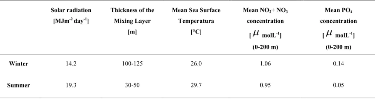
In situ samples made at the study site between 1978 and 1986 by Melo et al 1995, showed that during winter an intense vertical mixing is produced due to the decrease of the sea surface temperature and due to the increase of the intensity and persistence of winds and waves. This yields a thickening of the mixing layer up to around 110 m (Table 3) and favors the input of nutrients from deep waters into the euphotic zone, which yields higher levels of primary production (FERNÁNDEZ; CHIRINO 1993).

Moreover, during winter, incident solar radiation decreases (INSTITUTO DE GEOGRAFIA DE LA ACC; INSTITUTO CUBANO DE GEODESIA Y CARTOGRAFIA, 1989). According to Koblentz-Mishke et al. (1977), the chlorophyll content inside the cells increases with the decrease of incident solar radiation and with the increase of the concentrations of biogeochemical elements on the environment; both processes characterize the winter period.

During the summer, the increase of solar radiation and the decrease of the wind regime yield a thickening of the sea surface layer with strong thermal stratification, limiting the vertical mixing and

consequently the entrance of nutrients into the euphotic zone (CORREDOR, 1977). The thickness of the surface mixing layer is around 40 m (Table 6), and solar radiation reaches the highest values. At this season, despite the higher levels of phytoplankton concentration and biomass as reported by Perez et al.

(1990), the chlorophyll levels sensibly decrease as result of the decrease of nutrients on the mean and due to the increase of the incident solar radiation.

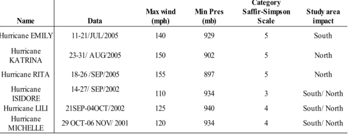
The positive peaks encountered on the series were mostly associated to extreme meteorological events. In the first period, between Jan-Mar/1998 the positive anomaly (Fig. 4) was especially high south of the island. García et al (1998) described the winter season between 1997 and 1998 as being very active, since 26 cold fronts reached Cuba due to the presence of ENSO. The authors also point out that a new record was established for the winter season, being February the most significant month due to the southern winds. Also Piñeiro (2004) express that 100% of front colds that affect the island pass through the zone C. Regarding cases II, III, and IV (Fig. 4), where the maximum values achieved were 0.04 mg/m3_{, 0,08} mg/m3 and 0,10 mg/m3, respectively, the positive anomalies were associated to a behavior described by Babin et al. (2004), as a response to the injection of nutrients and biogenic pigments on oligotrophic waters with the cooling of waters after the passage of hurricanes (Table 4). Walker (2005) describe that satellite-derived SST, SSH, and Chl a measurements clearly revealed rapid upwelling responses along and east of Ivan’s hurricane path where pre-existing cyclonic circulation experienced intensification. Venting of thermoclines and nutriclines can explain the SST cooling response of 3–7°C and subsequent Chl a enhancement.

Table 3. Seasonal behaviors of the main physical-chemical characteristics of the ocean waters around Cuba, according to Victoria et al. (1990).

Solar radiation

[MJm-2 _day-1_]

Thickness of the

Mixing Layer

[m]

Mean Sea Surface

Temperatura

[°C]

Mean NO2+ NO3

concentration

[

µ

(0-200 m)

Mean PO4

concentration

[

µ

(0-200 m)

Winter 14.2 100-125 26.0 1.06 0.14

Table 4. Hurricanes that pass through the Caribbean waters and affect monthly Chl a anomalies. (UNISYS, 2007).

Name Data

Hurricane EMILY 11-21/JUL/2005 140 929 5 South

23-31/ AUG/2005 150 902 5 North

Hurricane RITA 18-26 /SEP/2005 155 897 5 North

110 934 3 South/ North

Hurricane LILI 21SEP-04OCT/2002 125 940 4 South/ North

29 OCT-06 NOV/ 2001 120 934 4 South/ North

Max wind (mph)

Min Pres (mb)

Category Saffir-Simpson

Scale

Study area impact

Hurricane KATRINA

Hurricane ISIDORE

14-27/ SEP/2002

Hurricane MICHELLE

The increase of Chl a in June and July agrees with enrichment of the Caribbean waters by the Northern Brazil Current, which transports waters from the Amazon Plume and reaches the highest Chl a

values at this time of the year (0.5 to 5 mg/m3), as described by Pérez etal. (2004).

Fisheries

Cruz et al. (1990) established that the maximum captures occur after closed season due to the fisheries regimes with the country’s fishery management, they remain practically null during a 110 days period in order to protect animal breeding, growth and the incorporation of recruitments to the fishery. On the recalo period is observed a second peak because of the displacement of surface waters of the shelf, by the action of continuous intense winds during severe cold fronts, which can be responsible for the deeper and colder water entrance to the shelf, trigging massive lobster migrations towards the coast during winter (Baisre, 1994).

Figure 5 shows that the highest mean captures are obtained in the Zone B situated southeast of the island. This zone has the greatest fishing area (21,851.2 km2_{), and many authors point out that this} is the zone of greatest productivity due to the high availability of food, refuges, and environmental qualities (CRUZ et al., 1990; 1995; BAISRE; CRUZ, 1994; BAISRE et al., 1984; BAISRE, 2000, amongst others). The lowest captures occur in Zone C, which is situated on Northwest of the island and covers the smallest fishing area (3,438.5 km²). Baisre and Cruz (1994) state that the distribution of captures are related to the extension of the fishing zones, the mean depths, the fishing gears used, and the habitat and food availability.

Cross-correlation Coefficients

Taking into account the annual anomalies mean for each variable it was observed that cross-correlations coefficients reach highest values between Chl a and captures than for SST and captures. Mainly, positive correlations were determined for both variables, although there were some punctual negative significant correlation coefficient values for SST for 2 years of lagging in Zone C. Acording to Polovina et al. (2001), these oceanographic variables (SST and Chl a) are of critical importance in the early life history because of their hypothesized relationships to larval growth and feeding success, both critical precepts of larval survival and successful recruitment. It was shown in Figure 6, through the cross-correlation coefficient between Chl a and captures, how the food availability in the larvae stages might influence lobster captures.

higher than 0.2 mg m-3 indicate a presence of sufficient planktonic life to sustain a viable commercial fishing (GOWER, 1972).

In a monthly cross-correlation analysis, it was found that there are two significant periods for SST and captures coefficient, a positive correlation for western zones (B and C) in the winter months December and January for 1.5 years of lagging, while for the eastern zones this positive correlations occur in the summer months June and July also for 1.5 years of lagging. Looking for negative correlations between SST and captures originated a significant coefficient in October of 2 years of lagging for all study zones. Regarding Chl a and captures cross-correlation coefficient, each study zone had its own behavior. The maximum positive coefficient values were reached for all zones with 3 years of lagging, being the maximum values for zone B in November while maximum negatives were obtained for zones B and D for 1.5 years of lagging and to zone A and C for 2 years of lagging. Puga (2005) estimates that the mean ages of captured animals by fishing zones vary between 2.5 and 7 years, and they depend on the depth of the zone, the youngest catches occurring in zone D and the oldest in Zone A.

Sea surface temperature and chlorophyll a

concentration are widely available from a variety of satellite sensors, and both of these variables may have important linkages to the ecology of early life history stages, for growth and mortality (POLOVINA et al.

2001). Larval food supply involves spatial and temporal patchiness, and the species composition of the phytoplankton and microzooplankton is critically important (LASKER, 1975). In addition to starvation issues, variability in food supply has been shown to be an important determinant of larval growth and subsequent survival (BOOTH; ALQUEZAR, 2002). The correlation coefficients obtained leads to the reasoning that study environmental variables in the lobster life cycle would be more related to the larval phase that is developed in oceanic waters. This work corroborates the idea that significant correlation between these two environmental variables (SST and Chl a) measured by satellite with spiny lobster captures is important mainly for the planktonic life cycle of this specie in the Cuban waters.

A

Regla Duthit Somoza thanks the National Council of Technological and Scientific Development (CNPq), Brazil –for the scholarship which allowed the elaboration of this work during the International Course on Remote Sensing at INPE and to Milton Kampel for his patience as a tutor.

R

ALFONSO, I.; FRÍAS, M. P.; BAISRE, J.; HERNÁNDEZ, N.; PIÑEIRO R.; RODRÍGUEZ DEL REY, A. Distribución y abundancia de filosómas de Panulirus Argus y su relación con los factores hidrometeoro lógico. In: SIMPOSIO PLANTOLOGÍA' 99, 6-10 Sep. 1999, La Habana. Resúmenes... La Habana: [S.n.], 1999. 16 p. ARCE, A. M.; LEÓN, M. E. D. Biology. In: FAO/Western

Central Atlantic Fishery Commission. Report on the FAO/DANIDA/CFRAMP/WECAFC Regional Workshops on the Assessment of the Caribbean Spiny Lobster (Panulirusg argus). FAO Fish. Rept, n. 619, p. 17-25, 2001.

AUSTIN, H. M. Notes on the distribution of phyllosoma of the spiny lobster, Panulirus spp. in the Gulf of Mexico.

Proc. natn. Shellfish Ass., v. 62, p. 26–30, 1972.

BABIN, S. M.; CARTON, J. A.; DICKEY, T. D.; WIGGERT, J. D. Satellite evidence of hurricane-induced phytoplankton blooms in an oceanic desert. J. geophys.

Res., v. 109, C03043, 2004, WEB site

<10.1029/2003JC001938>.

BAISRE, J. A. Crónica de la pesca marítima en Cuba (1935-1995): Análisis de tendencias y del potencial pesquero.

In: FAO. Doc. Técn. Pesca, n. 394, 2000. 27p.

BAISRE, J.; CRUZ, R. The Cuban spiny lobster fishery. In: PHILLIPS, B. F.; COBB, J. S.; KITTAKA, J. (Ed.).

Spiny Lobster Management. Cambridge: University

Press, 1994. p. 119-132.

BAISRE, J.; GARCÍA, C.; CRUZ, R. Migraciones masivas de la langosta (Panulirus argus) en la plataforma Cubana. In: SIMPOSIO DE CIENCIAS DEL MAR Y VII JORNADA CIENTÍFICA DEL INSTITUTO DE OCEANOLOGÍA, 7, 5-9 nov. 1984, La Habana.

Resúmenes… La Habana, [S.n.], 1984. p 26-28.

BOOTH, D.J.; ALQUEZAR, R. A. Food supplementation increases larval growth, condition and survival of the brooding damselfish Acanthochromis polyacanthus (Pomacentridae). J. Fish Biol., v. 60:1126-1133, 2002. CALINSKY, M. D.; LYONS, W. G. Swimming behavior of

the puerulus of the spiny lobster Panulirus argus. J. crustacean Biol., v. 3, p. 329–335, 1983.

CIOTTI, A. M.; KAMPEL, M. Concurrent Observations of Ocean Color and Sea Surface Temperature between Cabo Frio e Cabo São Tomé. SIMPOSIO BRASILEIRO DE SENSORIAMENTO REMOTO, 10, Foz de Iguaçu, 21-26 April, 2001. Resumo… INPE, p 785-791, 2001. CORREDOR, J. E. Aspects of Phytoplankton dynamics in

the Caribbean sea and adjacent regions. Symposium on Progress in marine research in the Caribbean and adjacent regions. FAO, Fish Rep., n. 200, p. 101- 114, 1977.

CRUZ, R.; LEON, M. E. Dinámica reproductiva de la langosta (Panulirus argus) en el archipiélago Cubano.

Revta Investnes mar., Cuba, v. 12, n. 1-3, p. 234-245,

1991.

CRUZ, R.; BAISRE, J. A.; DÍAZ IGLESIAS, E.; BRITO, R.; GARCÍA, C.; CARRODEGUAS, C. Atlas Biológico-Pesquero de la Langosta en el archipiélago Cubano.

CRUZ, R.; LEON, M. E.; DÍAZ, E.; BRITO, R; PUGA, R. Reclutamiento de puérulos de langosta (Panulirus argus) a la plataforma Cubana. Revta Investnes mar., Cuba, v. 12, n. 1-3, p. 66-75, 1991.

CRUZ, R.; PUGA, R.; LEÓN, M. E. Prediction of commercial catches of the spiny lobster Panulirus argus in the Gulf of Batabano, Cuba. Crustaceana, v. 68, n.2, p. 238-244, 1995.

EHRHARDT, N. M. 2001. "Regional Review". In: FAO/Western Central Atlantic Fishery Commission. Report on the FAO/DANIDA/CFRAMP/WECAFC Regional Workshops on the Assessment of the Caribbean Spiny Lobster (Panulirus argus). FAO Fish. Rept, n. 619, p. 12-16, 2001.

FERNÁNDEZ, L.; CHIRINO, A. Atlas Oceanográfico del

Archipiélago Sabana-Camaguey. La Habana: Instituto

Cubano de Hidrografia, 1993.

FAO-FOOD AND AGRICULTURE ORGANIZATION (Ed.). Informe del segundo Taller sobre Manejo de las Pesquerías de la Langosta Espinosa del Área de la COPACO. La Habana, Cuba, 30 de septiembre - 4 de octubre de 2002. In: FAO Fish. Rept./FAO Infmes

Pesca, n. 715, 2003. 273 p. Web site:

<http://www.fao.org/

DOCREP/006/Y4931B/Y4931B00.HTM>.

GARCÍA, C.; HERNÁNDEZ, B.; BAISRE, J.; CRUZ, R. Factores climáticos en las pesquerías Cubanas de langosta (Panulirus argus): su relación con las migraciones masivas. Revta Investnes mar., Valparaiso, v. 12, n.1-3, p. 131-139, 1991.

GARCÍA, O.; BALLESTER, M.; LLANES, M.; NÚÑEZ A. R. Temporada Invernal de 1997-1998 en Cuba.

SOMETCUBA Bull., v. 4, n. 2, 1998. Web site:

<http://www.met.inf.cu/sometcuba/boletin/v04_n02/espa nol/tempora1.htm>

GORDON, H.R.; WANG, M. Retrieval of water-leaving radiance and aerosol optical Thickness over the oceans with SeaWiFS: a preliminary algorithm. Appl. Opt., v.33, p. 443-452, 1994.

GOWER, J.F.R. A survey of the uses of remote sensing from aircraft and satellite in oceanography and hydrography.

Pac.mar.Sci.Rept. Inst.Ocean.Sci., Sidney,B.C., p., 72–

73, 1972.

HERNÁNDEZ, B. Recalo 1986-1987 de la langosta (P. argus) en el Golfo de Batabanó. Revta Cubana

Investnes Pesq., v. 15, n. 1-4, 1988.

HERNANDÉZ, B. Variabilidad interanual de las anomalías de la temperatura superficial del mar en aguas Cubanas y su relación con eventos El Niño-Oscilación del Sur (ENOS). Revta Investnes mar., Valparaíso, v. 30, n. 2, p. 21-31, 2002.

HERNÁNDEZ, B.; PUGA, R. Influencia del fenómeno El Niño en la región occidental de Cuba y su impacto en la pesquería de langosta (Panulirus argus) del golfo de Batabanó. Revta Investnes mar. , Valparaiso, v. 23, p.3-24, 1995.

HERNÁNDEZ, B.; GARCÍA, C.; BAISRE, J. 1995. ¿Pueden los ciclones tropicales provocar migraciones masivas de langostas? Revta Cubana Investnes Pesq., v. 18, n. 3, p.23-25, 1995.

.INSTITUTO DE GEOGRAFÍA DE LA ACC; INSTITUTO CUBANO DE GEODESIA Y CARTOGRAFÍA (Ed.).

Nuevo Atlas Nacional de Cuba. La Habana, 1989.

KOBLENTZ MISHKE, O. I.; VEDERNIKOV, V. I.

Producción primaria. (en ruso) Oceanología. Biología

del Océano. Tomo 2. Moscu: Nauka, p. 183- 209, 1977. (In Russian).

LASKER, R. Field criteria for survival of anchovy larvae: The relation between inshore chlorophyll maximum layers and successful first feeding. Fish. Bull., v. 73, n. 3, p. 453-462, 1975.

MELO, G. N.; PÉREZ, R.; CERDEIRA, S. Variación espacio-temporal de los pigmentos del fitoplancton en zonas del Gran Caribe, a partir de imágenes de satélite Nimbus 7 (CZCS). Avicennia, v. 3, p. 103-116, 1995. MOREL, A. In-water and remote measurements of ocean

colour. Boundary Layer Meteorology, v.18, p. 177- 201, 1980.

MOREL, A.; PRIEUR, L. Analysis of variations in ocean color. Limnol. Oceanogr., v. 22, p. 709-722, 1977. LEÓN, M. E. DE; PUGA, R.; CRUZ, R. Panorama de la

pesquería de langosta en Cuba durante 1989. Revta

Cubana Investnes Pesq., v. 16, n. 3-4, p. 21-29, 1991.

LEÓN, M. E.; LÓPEZ, J.; LLUCH COTA, D.; HERNÁNDEZ, S.; PUGA, R. Decadal variability in growth of the Caribbean spiny lobster Panulirus argus (Decapoda: Paniluridae) in Cuban waters. Revta

Biol.Trop. , v. 53, n. 3/4, p. 475-486, 2005.

O'REILLEY, J.E.; MARITORENA, S.; O'BRIEN, M.C.; SIEGEL, D.A.; TOOLE, D.; MENZIES, D.; SMITH, R.C.; MUELLER, J.L.; MITCHELL, B. G.; KAHRU, M.; CHAVEZ, R P.; STRUTTON, P.; COTA, G.F.; HOOKER, S.B.; MCCLAIN, C.R.; CARDER, K.L.; MUELLER-KARGER, F.; HARDING, L.; MAGNUSION, A.; PHYNNEY, D.; MOORE, G.F.; AIKEN, J.; ARRIGO, K.R.; LETELIER, R.; CULVER, M. SeaWiFS Postlaunch Calibration and Validation Analyses. Part 3, Volume 11. In: HOOKER, S.B.; E. R. FIRESTONE, E.R. (Ed). NASA Tech. Memo. 2000-2206892. Greenbelt, Md: NASA Goddard Space Flight Center, 2000.

PÉREZ, R.; GIL, C.; LOZA, S. Variabilidad espacio-temporal del fitoplancton y sus pigmentos en aguas oceánicas al Sur de Cuba. Arch. Científ. Inst.

Oceanol. Acad. Cienc. Cuba, 1990.

PÉREZ, V.; FERNÁNDEZ, E.; MARAÑÓN, E.; SERRET, P.; GARCÍA-SOTO, C. Seasonal and interannual variability of chlorophyll a and primary production in the Equatorial Atlantic: in situ and remote sensing observations. J. Plankt. Res., v. 27 n. 2, p. 189 -197, 2004.

PIÑEIRO, R. Manejo integrado del recurso langosta en la

zona costera sur de pinar del rio. Disertación (Master

en Ciencias) - Centro de Investigaciones Marinas, Universidad de La Habana, La Habana, 89f. 2004. POLOVINA, J. J.; HOWELL, E. A.; KOBAYASHI, D.

R.; M.P. SEKI, M. P. The transition zone chlorophyll front, a dynamic global feature defining migration and forage habitat for marine resources. Progr. Oceanogr., v. 49, p. 469-483, 2001.

PUGA, R. Modelación bioeconómica y análisis de riesgo de la pesquería de langosta espinosa Panulirus argus

(Latreille, 1804) en el Golfo de Batabanó, Cuba. 2005.

SANTOS, A. M. P. Fisheries oceanography using satellite and airborne remote sensing methods: a review. Fish.

Oceanogr., v. 49, p. 1-20, 2000.

SOMOZA, R. D; KAMPEL, M.; SOUZA, R. B.; COBAS, S. Variabilidad de la temperatura superficial del mar obtenida a partir de imágenes AVHRR y su relación con las pesquerías de langosta (Panulirus argus) en las aguas Cubanas(1997-2004). Ambiente Água: An Interdisciplinary J. appl. Sci., v. 1, p. 6-20, 2006.

SOUZA, R. B. Introdução à oceanografia por satélites. In: (Org.). Oceanografia porSatélites. São Paulo: Oficina de Textos, 2005. vol. 1, p. 15-19.

STEWART, R. H. Methods of satellite oceanography. San Diego: Scripps Institution of Oceanography, 1985. 360 p.

VICTORIA, I.; CABAL, A.; GARCÍA, R.; HERNÁNDEZ, M.; PUENTES, H. Características oceanográficas de la Fosa de Jagua y de la zona económica exclusiva al Sur de Cuba . Informe final de Tema. Arch. Cientif. Inst. Oceanol. Acad. Cienc. Cuba, 1990.

TAVARES, M. Lobsters. (pp. 294-325) In: K. . Carpenter. (ed.). The living marine resources of the Western

Central Atlantic. FAO Species Identification guide for

fishery purposes and American Society of Ichthyologists and Herpetologists. Roma: FAO, 2002. 600 p. Spec. Publ. no. 5.

UNISYS. Atlantic Tropical Storm Tracking by Year. Available from http://weather.unisys.com/hurricane/atlantic/index.html, 2007.

WALKER, N. D.; LEBEN, R. R.; BALASUBRAMANIAN, S. Hurricane-forced upwelling and chlorophyll a enhancement within cold-core cyclones in the Gulf of Mexico. Geophys. Res. Lett., v. 32, 2005, L18610, doi:10.1029/ 2005GL023716. 2005.

YEUNG, C.; MCGOWAN, M. F. Differences in inshore-offshore and vertical distribution of phyllosoma larvae of Panulirus, Scyllarus, and Scyllarides in the Florida Keys in May–June, 1989. Bull. mar. Sci., v. 49, p. 699–714, 1991. ISI, CSA.

YEUNG, C.; LEE, T. Larval transport and retention of the spiny lobster, Panulirus argus, in the coastal zone of the Florida Keys, USA. Fish. Oceanogr., v. 11, n. 5, p. 286– 309, 2002.