Could cell membranes produce acoustic streaming? Making the case for synechococcus self-propulsion

Contents lists available atScienceDirect

Mathematical and Computer Modelling

journal homepage:www.elsevier.com/locate/mcm

Could cell membranes produce acoustic streaming? Making the case for

Synechococcus self-propulsion

Kurt M. Ehlers

a

, Jair Koiller

b,∗

a_{Truckee Meadows Community College, 7000 Dandini Blvd, Reno, NV 89512, USA}

b_{Centro de Matemática Aplicada, Fundação Getulio Vargas, Rio de Janeiro, RJ 22250-020, Brazil}

a r t i c l e i n f o

Article history:

Received 28 October 2009

Received in revised form 23 March 2010 Accepted 25 March 2010 Keywords: Acoustic streaming Microswimming Synechococcus MEMS devices

a b s t r a c t

Sir James Lighthill proposed in 1992 that acoustic streaming (AS) within the mammalian cochlea could play a role in the transmission of acoustic signals to the auditory sensory cells. Microelectromechanical devices for mixing and pumping, based on the acoustic stream-ing effect were introduced in the mid 1990s. Nature may have preceded this invention by 2.7 Gyr. We believe that acoustic streaming produced by nanometer scale membrane vibrations is widespread in cell biology. Flows generated by acoustic streaming could be produced along the ‘‘raphes’’ (central channels) of silica coated diatoms. Other possible in-stances are yeast cells and erythrocytes whose membranes generate nanoscale vibrations. We hypothesize that some of the most ancient organisms use acoustic streaming not only for self-propulsion but also to enhance their nutrient uptake. In this paper we focus on a motile strain of Synechococcus, a cyanobacterium whose mechanism for self-propulsion is not known. The calculations presented here show that a traveling surface acoustic wave (SAW) could account for the observed velocities. These SAWs would also produce a non-negligible Stokes layer surrounding the cell, motion within this region being essentially chaotic. Therefore, an AS mechanism would be biologically advantageous, enhancing local-ized diffusion processes and consequently, chemical reactions. Finally, we discuss possible experiments to support (or rule out) the AS model vs. other contending explanations for Synechococcus locomotion.

© 2010 Elsevier Ltd. All rights reserved. 1. Introduction

Acoustic streaming is the mean (rectified) flow resulting from the attenuation of an acoustic wave. Experimentally demon-strated by Faraday in 1831, a proof-of-concept for microfluidic applications was given in 1991 by Moroney, White and Howe [1]. (Moroney was then a graduate student at Berkeley.) Nowadays a thriving business exists for microelectrome-chanical (MEMS) pumps, valves and mixers using surface acoustic waves (SAWs) [2–5]. We call attention to the fact that, even in the low Reynolds number regime, there is a contribution from the inertial term of the Navier–Stokes equation when waves in the acoustic range are present.

Atomic force microscopy revealed that many cells generate membrane oscillations within the acoustic range. A couple (late) notes evoking Darwin’s year: filter feeding tunicates seem to rely on acoustic streaming for sensing and food harvesting. It has been suggested that outer hair cells (OHC) of mammals cochlea have copied (or evolved from) them about 600 million years ago [6]. Recently it has also been suggested that bats, whales, and dolphins use OHC piezoelectric properties directly in echolocation [7,8].

∗_{Corresponding author. Tel.: +55 21 37995910; fax: +55 21 37996091.} E-mail addresses:kehlers@tmcc.edu(K.M. Ehlers),jair.koiller@fgv.br(J. Koiller). 0895-7177/$ – see front matter©2010 Elsevier Ltd. All rights reserved.

Table 1

Possible AS parameters in the biological range.

Frequency (Hz) Amplitude (cm) Wave speed (cm/s) Power (W) η(%) Stokes layer (cm)

500 1.64×10−6 _{0.01 1×10}−15 _{1.17 1.78×10}−3

1000 1.16×10−6 _{0.02 2×10}−15 _{0.59 1.26×10}−3

1500 9.49×10−7 _{0.03 3×10}−15 _{0.39 1.00×10}−3

5000 5.20×10−7 _{0.10 1×10}−14 _{0.12 3.99×10}−3

This year marks the 50th anniversary of Richard Feynman’s famous Christmas talk at Caltech [9]. We think that he would like the idea of biological ‘‘samba loudspeakers’’. Feynman was fond of Brazilian carnival, in particular the instrument called ‘‘cuica’’, consisting of a drum with a short bamboo reed penetrating its head. Synechococcus may also be a ‘‘cuica’’ player. 1.1. Results: summary

We first discuss Lighthill’s paper on acoustic streaming in the inner ear [10] as many interesting questions remain open. We take the nerve to present some speculations on the controversial ‘‘cochlear amplifier’’ mechanism.

The main result of this paper is a model for self-propulsion of a microorganism based on acoustic streaming. A good candidate is the cyanobacterium Synechococcus which swims in open seas without flagella or other visible means of propulsion.1While translating, the cell rotates around its axis at about 1 Hz, see [11,12]. The mystery of Synechococcus motility is an outstanding problem, see e.g. [13].

We elaborate on two scenarios.2In the first, attenuation takes place in the body of the fluid, and the cell is pushed by the resulting flow. While the simplicity of this model is appealing, the power requirement seems too high to be biologically feasible, unless an enhancement mechanism is also present.

The second model employs a traveling SAW. Attenuation takes place in the Stokes boundary layer surrounding the cell. Employing this mechanism, a cell the size of Synechococcus can propel itself at observed speeds of 25 diameters per second using an

ω =

1

.

5 kHz traveling SAW with wavelength

λ =

10−5cm and amplitude 10−6cm. If this speculation is confirmed, Nature has scooped engineers by 2.7 Gyr.

All things being equal, AS is about 2.5 times more efficient than the ‘‘standard model’’ in which surface tangential deformations interact directly with the incompressible flow Stokes via no-slip boundary conditions. Moreover, acoustic streaming entails a mixing flow in the Stokes boundary layer, and this feature is biologically advantageous. For additional biological information we refer to the companion article [14].

The power output and efficiency for a cell of radius 10−4_{using boundary induced acoustic streaming to swim at 2}

_.

₅

_×

₁₀−3_, the observed speed of Synechococcus, is given inTable 1where we have (arbitrarily) chosen n

=

30.

1.2. Traditional microswimming modeling: Aristotelean physics

According to common wisdom, inertia plays absolutely no role in microswimming. This idea was beautifully explained by Purcell in a lecture given at the 1976 American Physics Society meeting [15]. However, if Synechococcus uses acoustic streaming for propulsion, it would be fair to say that these cells do actually know about Newton’s second law.3

The ‘‘textbook rule’’ is to use the incompressible Stokes equations with no-slip boundary conditions, imposing the constraint that a neutrally buoyant, free swimming organism does not exert net forces or torques on the surrounding fluid. This condition holds at each instant of time. As a consequence, if the swimmer retraces the stroke in reverse, no matter the time reparametrization, it returns to its initial position (the ‘‘scallop theorem’’ or ‘‘oyster paradox’’). In order to swim at zero Reynolds number, an organism or machine must possess at least two degrees of freedom, used in alternate cyclic order. For modern descriptions of this ‘‘gauge theory of something’’ see [20,21], and for a state of the art review, [18].

In practice, envelope deformation (squirming) models, first developed in the 1950s by Taylor and Lighthill, have been applied to ciliary propulsion. In this model the instantaneous shape of the organism is given by the locus of the tips of the cilia. One solves, quasi-statically, the Stokes equations with no-slip boundary conditions given by the instantaneous velocity field defined by the current deformation of a localized shape. To enforce the zero net force and torque one adds a counterflow, given by an infinitesimal translation and rotation. Cyclic but non-reciprocal boundary motions produce a net displacement through the fluid.

1.3. Breaking the paradigm: do cyanobacteria know that ‘‘f

=

ma’’ ?

Motile strains of the cyanobacteria Synechococcus were discovered in the Atlantic Ocean in 1985 [22]. Swimming at speeds of 10–25 diameters per second, their locomotion is unusual in that it does not involve flagella or other structures

1 Far from a oddity, Synechococcus, measured by total mass (=# organisms×mass/organism) outweighs all other species. 2 Announced in a preliminary version.

3 We review inAppendix Athe traditional approach [16–18]. InAppendix Bwe present the basic theoretical results on acoustic streaming, following Lighthill [19]. InAppendix Cwe apply the theory for streaming near a vibrating surface.

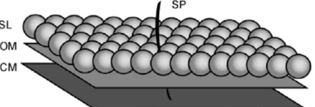
Fig. 1. Envelope structure of Synechococcus consisting of the cytoplasmic membrane (CM), the outer membrane (OM), and the crystalline surface layer (SL).

The SL is composed of SwmA arranged in a periodic rhomboidal pattern with 12-nm spacing between individual units [25,26]. The motile strain WH8113 could be covered with a forest of spicules (SP) [26] while strain WH8102 (also motile) lacks spicules [25].

typically associated with bacterial motility. Both sodium and calcium are required for motility [23]. A glycoprotein, swmA, forms a crystalline surface layer (‘‘S-layer’’) on motile strains. Both swmA and another protein, swmB (which is also localized near the cell surface), are necessary for motility [24]. While photosynthetic, as are all cyanobacteria, motile strains of Synechococcus do not show a phototactic or photophobic response to light, but do show a chemotactic response to certain nitrogenous compounds. For more biological details, see [14].

We suggest that Synechococcus could be using acoustic streaming (AS) for self-propulsion (Fig. 1). We emphasize that this employs an entirely different physical principle than the usual paradigm.Like the squirming model, small amplitude cyclical motions along the outer membrane are rectified into mean streaming flow. The difference lies in the underlying physics. In the AS model the membrane oscillations produce a surface acoustic wave. It is the wave–fluid interaction that produces the streaming flow. The inertial term of the Navier–Stokes equations that is ignored in previous models of microswimming is relevant, as is the fact that water has some degree of compressibility.

In a symmetric setting, a standing wave generates a mean rotational flow near the membrane which, for instance, can be used for enhancing nutrient uptake. In an asymmetric geometry, even a standing (hence reversible) wave could produce locomotion, in flagrant violation of the scallop theorem.

2. Essentials of acoustic streaming

2.1. A bit of history: acoustic streaming and the piezoelectric effect

Although there is just a note on the subject in his celebrated 1877 Theory of Sound [27], a few years later Lord Rayleigh provided a theoretical foundation for acoustic streaming, in an analysis of Kundt’s tubes [28]. Rayleigh also wrote an important paper on solid/fluid interactions [29]. After a long period of dormancy, Nyborg (and others) revived acoustic streaming in the 1950s, motivated by the emerging area of medical ultrasound (see [30] for a recent review article).

Also around 1880 properties of piezoelectric crystals where being studied by Pierre Curie and his older brother Jacques. Piezoelectric materials convert mechanical deformations into voltage differences, and vice versa, providing a wonderful form of energy transduction. The piezoelectric effect was regarded as a curiosity at that time. Nowadays, its applications range from door buzzers, microphones and electric guitar pick-ups, to auto-focus cameras, sensors in cars, aeronautical and space instrumentation, and is fast moving into nanotechnology.

2.2. Physics of acoustic streaming

Acoustic streaming is a subtle, nonlinear, second order effect. As we mentioned before, in traditional microswimming modeling (Appendix A), water is assumed to be incompressible. In contradistinction, acoustic streaming takes into account that the fluid has some degree of compressibility, as we discuss inAppendix B. Even for highly viscous flows part of the inertial term in the Navier–Stokes equation must be retained. In his 1978 review [31], Lighthill describes the theory of acoustic streaming in both low and high Reynolds number regimes. Later, Riley presented a somewhat broader view called

steady streaming [32]. The low Reynolds number situation, which is appropriate for our purposes, is called RNW streaming

after Rayleigh, Nyborg and Westervelt. See also the classic paper by Longuet-Higgins [33].

Acoustic streaming is the mean steady flow in a fluid induced by the oscillatory fluid motions of a sound wave. This phenomena was recognized by Faraday in 1831 who noticed that air currents above a vibrating plate flow towards the nodes where the displacement is zero and away from the antinodes where the displacement is maximum [34]. The steady flow is forced by a gradient in the mean momentum flux created by attenuation of the sound wave. The attenuation of the acoustic wave necessary for mean streaming can take place in the body of the fluid or next to solid boundaries.

It was shown by Lord Rayleigh that the mean rate of momentum flow across a unit area acts as a force per unit area [27] which is now referred to as the Reynolds stress. For an oscillating velocity field with components ui(i

=

1

,

2

,

3) in a fluid region with coordinates xi, the Reynolds stress tensor

τ

has components

τ

ij

=

ρ

uiuj. The bar represents the time average taken over many cycles. The component

τ

ijrepresents the mean flux of the xj-momentum per unit volume (

ρ

uj) in the

xidirection. The mean force acting on a fluid element is then given by the gradient of

τ

. The mean streaming velocity is found by solving the Navier–Stokes equations with an applied force given by the gradient of the Reynolds stress tensor. (SeeAppendix Bfor additional mathematical details.)

In [19], Lighthill emphasizes that a gradient in

τ

leads to streaming only if the acoustic wave is attenuated. Here attenuation is the fraction of acoustic energy lost per unit of propagation length. The attenuation necessary for streaming can occur in the body of the fluid or in a Stokes boundary layer surrounding a surface. Acoustic streaming due to attenuation in the body of the fluid can be observed when a quartz crystal is electrically excited, producing high frequency vibrations via the piezoelectric effect. This is commonly called a quartz wind (QW). In air, jets with speeds of up to 10 cm/s can be generated in front of the face of a quartz crystal. In Lighthill’s words, ‘‘not only can a jet generate sound, but also sound can generate a jet’’. Attenuation in the body of a fluid is proportional to the square of the frequency and it is for powerful high frequency (typically ultrasonic) sound sources that the QW effect causes significant streaming velocities.

The second form of AS occurs near boundaries. Here the attenuation of the sound wave is a result of strong shear stresses within the Stokes boundary layer. If U is an oscillating velocity field in a fluid, then this layer is the region surrounding the surface where the bulk flow vorticity is non-zero; the streaming flow is irrotational outside this layer. The effective thickness of the Stokes boundary layer is 5

(ν/ω)

1/2_where

_ν

_{is the kinematic viscosity and}

_ω

_{is the frequency of U (see} Fig. C.8). Boundary induced streaming can be generated either by a acoustic wave in the fluid or vibrations of the boundary itself; the streaming is a result of relative motion. As calculated by Rayleigh, the resulting velocity is second order in the wave amplitude and independent of the viscosity (even though the attenuation is a result of the viscosity). A traveling acoustic wave leads to a mean streaming velocity parallel to the boundary while a standing wave leads to streaming away from the antinodes and towards the nodes as observed by Faraday.

Summarizing: outside the Stokes layer flow is laminar and irrotational. Within the Stokes layer, the flow is turbulent and rotational. We can poetically imagine a chaotic ‘‘fluid atmosphere’’ surrounding the cell. Our calculations indicate that, surprisingly, the Stokes layer’s thickness is non-negligible for a singing cell.

2.3. Possible instances of acoustic streaming in cell biology

Acoustic streaming MEMS systems are nowadays a standard tool for bioassays: fluids can be easily pumped or mixed in the microscale.

Therefore, Nature must have taken advantage of acoustic streaming. However, as far as we know, the only situation for which AS has been explicitly proposed is in Lighthill’s cochlear model.

Three recent cell biology findings were eye-opening to us:

1. In [25,26], deep-freeze electron microscopy of the motile Synechococcus strains 8102 and 8113 revealed the presence of a crystalline outer ‘‘S-layer’’. In the latter, a forest of ‘‘spicules’’ was also observed, extending from the inner membrane, and projecting 150 nm into the surrounding fluid.4_{In the former, mutant cells lacking the outer S-layer, composed of}

swmA, do not swim (when accidentally attached to a slide, however, they still rotate).

2. Using atomic force microscopy (AFM), the outer membranes of Yeast cells have been observed to oscillate at between 0.8–1.6 kHz with typical amplitudes of

∼

3 nm [35]. The oscillations were shown to be driven by molecular motors.5The magnitude of the forces at the cell wall were measured to be

∼

10 nN suggesting that they are generated by many protein motors working cooperatively.

3. In [36], quantitative phase imaging (QFI) was used to detect nanoscale vibrations of the order of 200 nm in red blood cells.

We could also add diatoms to this list. These organisms come up after cyanobacteria in the tree of life. Diatoms are very popular among bioengineers, since they are basically of the same size, shape and material as microchips (and very cheap to produce — the ideal template). We speculate that they could use acoustic streaming to pump fluid along their raphe, a microchannel in their crystalline surface. For basic information, see [37] and the special issue on diatom nanotechnology [38]. 3. Lighthill’s cochlear model and its possible developments

Sir James Lighthill has suggested that acoustic streaming within the fluid filled cochlea may play a role in mammalian hearing [10]. In this model, acoustic streaming in the cochlea resulting from localized oscillations of the basilar membrane induces a flow sufficient to deflect the stereocilia of the inner hair cells. When the stereocilia are deflected an electric signal encoding the sound wave is sent to the brain.

3.1. Physiology: outer and inner ear structures

Sound waves collected by the auricle of the outer ear pass through the auditory canal striking the tympanic membrane (eardrum). The sound wave is transmitted through the middle ear via the ossicles consisting of three delicate bones: the hammer that is in contact with the tympanic membrane, the anvil, and the stirrup which is in contact with the oval window of the cochlea (Fig. 2).

4 There are some doubts about the existence of the spicules: they may have been artifacts of the preparation of the specimens for electron microscopy. They are not necessary to our model, but are helpful.

5 Since the 1970s, power source systems have been identified for intracellular transport (kinesin molecular motors), locomotion systems for bacteria (protonmotive rotary motors), and protozoa (dynein motors distributed along the axonemes).

Fig. 2. The basic layout of the human ear. Sound waves transmitted through the bone of the middle ear enter the cochlea through the oval window.

The membrane of the round window moves in the opposite direction of that of the oval window and is necessary because of the incompressibility of the cochlear fluids.

Fig. 3. Simplified diagram of an uncoiled cochlea. Characteristic places for high frequencies are near the base of the cochlea and characteristic places for low

frequencies are near the apex. Sound waves entering the cochlea induce a traveling wave along the basilar membrane. The wave speed slows dramatically at the characteristic place for the frequency. The spatial wavelength shortens and the amplitude increases to a peak then falls off precipitously.

Vibrations of the stirrup on the oval window cause a traveling wave within the fluids of the cochlea. In the cochlea, sounds are decomposed into their component frequencies, converted into an electrical signal and transmitted to the brain. The cochlea is shaped like the shell of a snail with 2 1

/

2 turns, and consists of three fluid filled sections: the scala vestibuli, the scala tympani and the scala media. The scala vestibuli and scala tympani are filled with a fluid called perilymph and are connected at the apex of the cochlea. The scala media is partitioned from the scala vestibuli by the Reissner’s membrane and from the scala tympani by the basilar membrane and is filled with a fluid called endolymph with a high concentration of positively charged potassium ions. Sitting atop the basilar membrane (within the scala media) is the organ of Corti which converts the mechanical sound wave into an electrical signal.

The key to the ability of the ear to decompose frequencies is the structure of the basilar membrane. Each position along its length is tuned to a particular frequency. Near the oval window it is narrow and stiff being tuned to high frequencies. Near the apex of the cochlear duct it is tuned to low frequencies being wide and compliant. The stiffness decreases by four orders of magnitude from the base to the apex. The basilar membrane is constructed of radial fibers allowing a particular place to oscillate nearly independently of nearby places.

The organ of Corti has two type of hair cell: outer hair cells (involved with the cochlear amplifier) and inner hair cells. The inner hair cells of the organ of Corti act as sensory receptors. Each hair cell has approximately 300 ‘‘hairs’’ called stereocilia. A hair cell normally carries a voltage potential across its outer membrane but if the stereocilia are deflected, positive ions of the endolymph are allowed to enter causing depolarization of the cell. This sets off a chain of events resulting in an electric signal being sent to the brain(Fig. 3).

A great deal of biological information has been obtained recently [39], motivating a boom of theoretical work, with very different approaches. In what follows we admittedly go very bare.

3.2. Lighthill’s model: acoustic streaming in the cochlea

Sound waves transmitted to the cochlea induce a traveling wave along the basilar membrane. As the traveling wave approaches the characteristic place for the particular frequency

ω

its phase speed c slows, its spatial wavelength

λ =

2

π

c

/ω

shrinks, and its amplitude V increases to a peak before precipitously dropping. The wave energy per unit length E reaches a maximum Emaxat this characteristic place.

In addition to this passive system for frequency discrimination, mammals have evolved a remarkable cochlear amplifier that both increases the amplitude at the characteristic place and localizes the peak [39]. Amplification, which is between 20 and 30 decibels, results from motility of the outer hair cells of the organ of Corti in response to a positive feedback control system. The precise workings of this active system of amplification are the subject of intense debate. The cochlear amplifier allows mammals hear nuances of speech and music over a wide dynamic range of intensity. Any streaming velocities of the endolymph would also enhanced by the amplification.

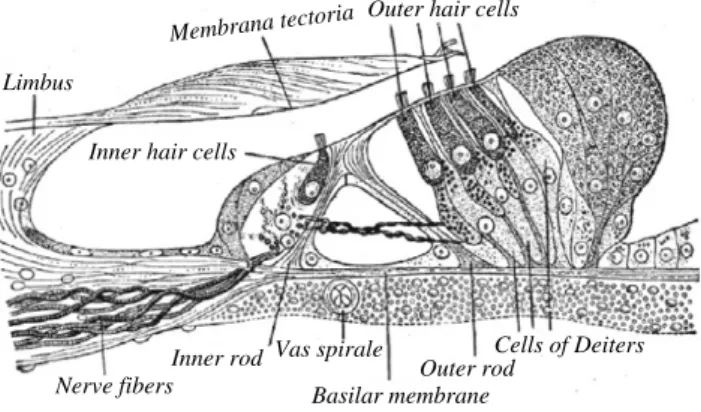
Limbus

Outer hair cells

Inner hair cells

Inner rod _{Outer rod}

Basilar membrane Vas spirale

Nerve fibers

Cells of Deiters Membrana tectoria

Fig. 4. The Organ of Corti (Gray’s anatomy classical figure). The inner hair cells are responsible for converting the mechanical action of a sound wave to

an electrical signal. The outer hair cells are involved in the mammalian cochlear amplifier.

While the hairs of the outer hair cells are deflected by direct contact with the tectorial membrane (seeFig. 4), inner hair cells are deflected by motions of the endolymph itself. This is where acoustic streaming could play a role. In his 1992 paper Acoustic streaming in the ear itself [10] Lighthill shows that significant acoustic streaming with velocity

1 4V

2_c−1

₋

3

4V

(

dV

/

dx

)ω

−1 ₍₁₎

occurs near the characteristic place. Here

(

V

(

x

),

0

,

0

)

is the velocity amplitude of the basilar membrane’s vibration. Recall that at the characteristic place, the phase speed c of the traveling wave rapidly diminishes to zero while the amplitude increases, greatly enhancing the local streaming velocity. Lighthill estimates that, near the characteristic place, the volume outflow per unit length along the basilar membrane is

0

.

015Emax

ρ

L

√

ων

(2)

where

ρ

is the density and

ν

is the kinematic viscosity of the endolymph (these are essentially those of pure water). L is the

e-folding distance of the stiffness of the basilar membrane (the distance over which the stiffness decreases by 1

/

e

=

37%

of its original value, approximately 6–7 mm for a human cochlea). If the cross sectional geometry of the scala media causes the streaming flow q to be channelled between the organ of Corti and the tectorial membrane, the stereocilia of the outer hair cells could be also deflected by the throughflow.

3.3. Open questions

Lighthill, who died in 1998 while swimming around the island of Sark (one of his favorite past times), did not publish his planned sequel. Several important open questions are:

•

Is the streaming flow q channelled through the space between the tectorial membrane and the inner hair cells?

•

If so, what is the resulting force exerted on the stereocilia?

•

How is streaming enhanced by the action of the outer hair cells?

The first question seems to have been answered positively, see [40]. Fluid mediated communication between inner and outer hair cells may occur also in the Corti tunnel, see [41].

We finish this section outlining one possibility for a positive feedback loop. We do not claim originality nor correctness, as the ‘‘grand picture’’ for the cochlear amplifier mechanism is in order.

1. External sound waves enter the oval window. Acoustic streaming along certain places of the basilar membranes set endolymph fluid into motion.

2. This motion induces deflections of the inner and outer hair cell’s stereocilia opening channels that trigger electric signals to the brain.

3. As the outer hair cells receive these signals, prestin6is activated, making the cells oscillate longitudinally.

4. These oscillations deflect the outer hair cells stereocilia. The channel flow (called q) is enhanced, again by acoustic streaming, or via the tectorial membrane motion. We get more endolymph fluid motion.

5. This enhanced endolymph fluid motion enters in loop with step 1.

4. Acoustic streaming in microswimming

We now turn to the main part of the paper. We begin with an estimate of the streaming velocity associated with the oscillatory motion of a yeast cell, using the parameters found by Pelling [35]. According to Rayleigh’s classical result, for a standing wave with velocity U

(

x

)

eiωt, the local streaming is given by (seeAppendix Afor a discussion of this formula)

UL

= −

3 4

ω

U

(

x

)

U ′

₍

x

).

(3) We take U

(

x

) =

0

.

003

(

1500

π)

sin

(

2

π

x

)

(4)

corresponding to a 1.5 kHz vibration with a 3 nm amplitude. We have (arbitrarily) taken the spatial wavelength to be one micron. The streaming velocity is approximately

−

0

.

1 sin

(

2x

) µ

m

/

s

.

(5)

We note that the streaming velocity is directed away from the antinodes and towards the nodes and is not propulsive. Nonetheless, the rotational streaming velocities in the fluid near the cell membrane should enhance cell chemistry through local mixing.

We now present two scenarios for locomotion involving acoustic streaming. The first one has, in fact, been used for propelling an experimental underwater vehicle,7but it is not efficient in the low Reynolds regime. The second scenario, on the other hand, is quite competitive, as we now report.

4.1. Quartz wind model

In this simplest model, attenuation of the acoustic beam in the bulk of the fluid generates a flow, pushing the organism through the fluid.8

Here is a ‘‘back of the envelope’’ computation: Stokes’ law F

=

6

πµ

a

v

gives the force required to push a sphere of radius a through a fluid with viscosity

µ

at speed

v

. Lighthill [19,43] argues that the force (F ) is related to the acoustic power (P) and the speed of sound in the fluid

(

c

)

by

F

=

P

/

c

.

(6)

The necessary acoustic power is then

P

=

6

πµ

a

v

c

.

(7)

Synechococcus has a radius of about 10−4cm and swims in sea water (viscosity 10−2g

/

cm s) at about 2

.

5

×

10−3cm

/

s. It would therefore require about 7

×

10−10W of acoustic power to drive Synechococcus at observed speeds. By comparison, the power needed to push the cell is 6

πµ

a

v

2_{or approximately 1}

_.

₁₈

_×

₁₀−17_{W. Lighthill [44] defines an efficiency}

_η

_{for a} swimming mechanism as the inverse ratio of the power required to push the cell to the power required by the mechanism:

η =

6

πµ

a

v

2

/

P

.

(8)

By this definition, the efficiency of the quartz wind mechanism is only about

1

.

7

×

10−6

.

(9)

The acoustic power necessary for an organism to swim using this mechanism might be unrealistically high. In the discussion we speculate on possible power output enhancement mechanisms.

4.2. Boundary induced streaming: surface acoustic waves

In this model a high frequency traveling SAW passes along the crystalline outer S-layer of the cell leading to boundary induced streaming. The vibration is (literally!) piezoelectrically transduced by molecular motors. Spicules, if present, help attenuation and/or to provide sound guidance. The progressive acoustic wave induces a steady slip-velocity at the outer edge of the Stokes boundary layer.

We found that Lighthill’s efficiency for boundary induced streaming approaches 1%, comparing favorably with the squirming and flagellar propulsion strategies. The amplitude of the SAW necessary to drive an organism the size of Synechococcus at observed speeds is on the order of 10−7_{cm, too small to be resolved using light microscopy.}

We estimate the velocity and efficiency for a spherical cell that swims using a traveling SAW. For simplicity, we consider a tangential SAW (though a normal SAW would also lead to self-propulsion). We compute the streaming velocity and the

7_{http://censam.mit.edu/news/posters/hover/1.pdf.}

8 We wonder of spicules could also help, by pushing and pulling the S-layer in the manner of the Brazilian samba instrument known as ‘‘cuica’’, consisting of a drum with a short bamboo reed penetrating its head.

power output (per unit area) for a swimming slab, then use these results to estimate the swimming velocity and power output for a spherical organism. This ‘‘tangent plane approximation’’ was proposed in [20] for estimates in the traditional microswimming approach. It provides a good estimate when the wavelength of the SAW is much smaller than the radius of the cell.

Consider a slab of infinite extent with coordinates

(

x

,

y

)

bounding an infinite region of water in the region z

≥

0. Suppose tangential progressive waves pass along the slab in the

+

x-direction with

xm

=

x

+

A sin

(

nx

−

ω

t

)

(10)

where xmis a material line on the slab.

The streaming velocity just outside the Stokes layer is then U

= −

A

ω

cos

(

nx

−

ω

t

)

. The streaming velocity at the edge of the Stokes layer is then

UL

= −

5

π

2

λ

ω

A

2 ₍₁₁₎

where

λ =

2

π/

n is the wavelength (seeAppendix Afor a derivation of this formula).

Now consider a spherical organism of radius r that swims by passing high frequency traveling compression waves along its outer membrane. Let

(θ, φ)

be spherical coordinates with

φ

the azimuthal coordinate measured from the front of the organism. Take the wave to be

φ

m

=

φ + ϵ

sin

(

n

φ − ω

t

)

(12)

where

φ

mrepresents a material point on the outer membrane. The amplitude of the velocity is A

=

ϵ

r

ω

and the wavelength is

λ =

2

π

r

/

n. We assume that

λ ≪

r so that the local streaming velocity is well approximated by(11). In this case, we take as a slip-velocity

U

=

5

4n

ωϵ

2_i

φ (13)

where i_φis the unit vector in the direction of the azimuthal spherical coordinate at the surface of the cell.

A convenient formula for the translational velocity associated with any boundary velocity field was derived using the Lorentz reciprocity theorem in [45,17], which, for a sphere is

A

(

U

) = −

1 4

π

r2

∫

∫

S

UdS (14)

where the integral is taken over the surface of the sphere. Evaluating this with velocity(13)we find that the spherical organism swims with velocity

5 16

π

nr

ωϵ

2 ₍₁₅₎

along the axis of symmetry. Note that the amplitude of the SAW is r

ϵ

and

ω =

2

π

f where f is measured in Hertz. Written in terms of wavelength and phase velocity of the traveling wave c

=

λν

this velocity can be written

(

5

π

3

/

4

)(ϵ/λ)

2c

.

(16)

This is 2.5 times the velocity predicted by the squirming mechanism all parameters being equal [16]. 4.3. Efficiency of the SAW mechanism

To estimate the effort required to execute the compression waves we compute the power P

=

∫

∫

S

v

i

σ

ijdSj (17)

averaged over a swimming stroke. Again we assume

λ ≪

a and approximate the average power using the average power per unit area for a waving sheet. For a sheet in the xy-plane with a fluid of viscosity

µ

filling the region z

≥

0, the average power per unit area necessary to deform according to

xm

=

x

+

A sin

(

kx

−

ω

t

)

(18)

is

2

πµω

2A2

/λ

(19)

where

λ =

2

π/

k, see [46]. For the sphere deforming according to(12)we have A

=

r

ϵ

and

λ =

2

π

r

/

k. Substituting these into(19)and multiplying by the area we arrive at

P

=

4

πµ

r3n

ω

2

ϵ

2

.

(20)

We note that this expression is in good agreement with the result obtained by evaluating(17)in spherical coordinates for large n; for instance, when n

=

10 the actual coefficient is 4.04.

5. Discussion

The quartz wind strategy is less efficient by many orders of magnitude and is probably not biologically feasible unless some mechanism for power enhancement is present. On the other hand, all things being equal, propulsion by surface acoustic waves predicts a swimming velocity 2.5 times that predicted by squirming. At any rate, a theoretical model for how cells can generate high frequency oscillations using coupled molecular motors has been developed by Jülicher [47], predicting that molecular motors working in unison can produce cellular oscillations with frequencies of 10 kHz and beyond.

If these molecular motors produce an helical wave, or the S-layer has a helical ribbon attached to it, the cell would rotate as it translates (‘‘drilling motion’’) as reported in the initial observations by Waterbury et al. [22].

For Synechococcus, the required frequency of the SAW is within the range observed in other biological systems. The amplitude required for observed speeds is on the order of 10−6_{cm, below the resolution limit of light microscopy. This} leads to the key questions. If acoustic streaming generated by surface acoustic waves is responsible for the locomotion of Synechococcus, how could we ‘‘listen to their songs’’? Are there alternative explanations?

5.1. Contending explanations

Acoustic streaming models presented here refine the previous model by Ehlers et al. [16] in which the traditional microswimming modeling is applied to an organism or robot capable of producing tangential compression–expansion waves of submicron amplitudes on its physical membrane. We argue that for vibrations in the nanometer scale AS gives the correct Physics.

As far as we know, so far the only published alternative explanation for Synechococcus locomotion was given by Samuel et al. [26]. Recall that Synechococcus has an external crystalline shell (S-layer). In their fast-freezing electronic microscopy study, Samuel and coworkers observed a forest of ‘‘spicules’’ (too small to be observed by optical microscopy). They hypothesized that these projections could perform rowing motions. However, in her Ph.D. dissertation McCarren reported that she found no spicules and suggested that these could be artifacts of preparation [11].

As this paper was being revised, we learned from Richard Montgomery about other contending models for Synechococcus swimming being considered by George Oster’s group, building upon models they and others developed for Myxobacteria gliding (see [48–50]). Recently, a new molecular motor involved in the gliding motility of Mycoplasma mobile was discovered, [51–53]. George Oster speculates that similar (but yet uncharacterized) motors could be involved in Synechococcus swimming.

For Myxobacteria, Oster and collaborators showed how these motors, distributed along the cell body could coordinate to produce the so-called A (‘‘adventurous’’) gliding [54,55]. In one of their models, the motors would drive a helical rotor structure inside the cell at about 6 revolutions per minute. As the internal structure reverses direction, the cell reverses its direction of motion about every 6 min.

For Synechococcus swimming, motor stators spanning the inner membrane would drive an ‘‘egg-beater’’ rotating structure inside the cytoplasm. In analogy to Spirochetes, where an internal flagellum hidden in the periplasmic space [56] makes the entire cell counter-rotate, the Synechococcus outer shell would counter-rotate relative to the inner membrane (but much faster since the viscosity of the cytoplasm in which the helix spins is 103_{times as viscous as water). In this} model, the S-layer has a passive role, but if it has an attached spherical helix ribbon (or carved grooves) the cell would move ‘‘drilling’’ through the water.9_{We speculate that the new type of molecular motor could function as ‘‘percussion beaters’’ in}

our acoustic streaming models, providing even a role for the purported spicules.

A collaboration (KE) with Oster’s group to explore these avenues is being considered. It would be important to estimate the efficiency of the latter mechanism in order to compare with our acoustic streaming model.

5.2. Possible experiments

It is a bit far-fetched, but perhaps the thylakoid membrane (an unique feature of cyanobacteria, where photosynthesis occurs), could work as the purported ‘‘egg-beater’’ internal rotating structure. It was recently found that the thylakoid membranes form a continuous structure, actually resembling (in the view of a mathematician) a closed Riemann surface (of high genus). The holes in the donut allow cytoplasmatic flow. Some relevant references are [57–59]. We believe that this surrogate of Oster’s proposal could be tested placing markers along the thylakoid structure to verify if it is indeed counter-rotating relative to the outer shell. This would also give a mechanical role for the not fully understood thylakoid centers, where the thylakoid membrane branches attach (ramification points in the mathematician’s view). We refer to the companion paper [14] for many other recent and exciting biological findings.

The ‘‘holy grail’’ would be to identify the molecular motor responsible for Synechococcus locomotion, the ultrastructural features of the locomotion machinery and, perhaps most importantly, understanding in a ‘‘cartoon’’ the mechanical process going on. Prestin, the outer hair cell molecular motor identified in 2000, functions like piezoelectric transducer. Will a

similar molecular motor be found for Synechococcus? (Gliding cyanobacteria contain a glycoprotein, oscillin, which has some homology to swmA, but both seem to have a passive role in locomotion.) Here we suggest some physical experiments based on recent developments in nanotechnology.

AS nanosensors: listening to the sound of cells. Can one ‘‘hear’’ the sound generated by a moving Synechococcus, via nanosen-sors attached to the crystalline shell? Cantilever/nanowire devices are already available that can measure piezoelectric dis-placement transduction whose frequency and amplitude approach the quantum regime.

Pelling, et al. measured periodic oscillations with amplitudes of 3 nm at frequencies of 0.8–1.6 kHz on the of the outer membrane of Yeast cells using the cantilever of an atomic force microscope [35]. Living Yeast cells that measure about 5

µ

m in diameter were trapped in the micro-pores of a filter for the experiment. Yeast cells were chosen for the experiment due to their stiff cell wall; the spring constant of the cantilever needs to be comparable to the spring constant of the cells wall. Could this experiment be adapted to ‘‘listen’’ a Synechococcus? For the state of the art on AS sensors at the microscopic realm we refer to a recent review paper [60]. Other recent microscopy techniques are environmental scanning electron microscopy10[61,62] and piezoresponse force microscopy [63].

Direct visualization/manipulation of the flow. We believe it possible to map the flow pattern of the fluid adjacent to a swim-ming cell using technologies such as total internal reflection velocimetry (TIRV, see the review [64]). By 2011 it is expected that particles of 25 nm will be able to be manipulated on chips, see International Technology Roadmap for Semiconductors http://www.itrs.net/.

The observed flow via TIRV could be matched with the characteristics of acoustic streaming induced flow. Detailed analysis of the fluid mechanics and careful experimentation would be required in the case of a progressive (propulsive) SAW. A very interesting and challenging mathematical problem is to model the chaotic flow pattern inside the ‘‘atmosphere’’ (the Stokes layer) surrounding the cell. Note that our estimates showed that it is non-negligible.11

We note that experiments on diatoms should be simpler to do. Fluorescent beads inside the raphe could be focused by a standing SAW. Certainly some of the techniques described in [60] could be applied to a diatom skeleton to probe its piezo/mechanical properties.

5.3. Physical effects related to AS

Quartz wind enhancement: uasers. Quartz wind is a very simple mechanism, but it is inefficient in the low Reynolds regime. One way to remedy this drawback is to imagine a power enhancement mechanism similar to a laser. Uasers [65] are coupled ultrasonic transducers producing stimulated emission via positive feedback with an internal power mechanism. Power output scales with the square of the number of oscillators, and one could try to find signs of phase locked excitations (a samba school ‘‘cuica’’ orchestra).

Streaming flow enhancement by submicrobubbles. Nyborg pointed out, many years ago, that an external ultrasound source resonating immersed bubbles adjacent to a cell could induce internal cellular processes. Conversely, acoustic waves produced by the cell could resonate submicrobubbles attracted to the crystalline layer, enhancing the streaming flows. Experiments with inorganic materials have confirmed this effect [4,66].

Cavitation energy. Lord Rayleigh studied the deleterious effects of cavitation on ship propellers. In medical ultrasound care must be taken to avoid tissue damage caused by cavitation, but it may also be used to perform microsurgeries or to insert biological materials into cells. One could speculate on a locomotion model based on direct extraction of energy stored in submicrobubbles, perhaps coupled to some ratchet type mechanism. Moreover, in the process of bubble collapse, several chemical reactions occur [67]. A curious coincidence is that chemical reactions involving nitrogenous compounds are commonly produced in bubble cavitation. This may be of interest since Synechococcus is attracted to nitrogen. Hydrophylic/hydrophobic transitions. Micro-engineered surfaces coated with nanonails, when charged, exhibit controlled hydrophylic–hydrophobic transitions [68]. One can speculate that an hydrophylic–hydrophobic wave could entrain pumping motions, mediated perhaps by some ratchet type asymmetry or bubble manipulation. This is another suggestive clue, since the spicules project 0

.

15

µ

m to the exterior of the crystalline shell. Devices with chemically induced hydrophylic–hydrophobic microtracks have been recently constructed [69,5].

5.4. Mathematical directions

A somewhat simpler but nonetheless intriguing viewpoint for acoustic streaming has been proposed in [70]. In order to estimate the streaming flow inside a spherical cavity, ‘‘vorticity boundary conditions’’ were applied directly to the incompressible Stokes equations. In our setting, one would consider the external flow.

In a similar vein, the ‘‘blinking stokeslets’’ proposed by Blake and coworkers [71] can be reinterpreted as true ‘‘physical’’ generators of the acoustic wave. This approach is appealing as it connects directly with the membrane force generators. 10 One advantage is that it does not require a vacuum and can be used on wet biological samples

11 Prof. Howard Berg (personal communications) tried to visualize the flow with particles under common microscopy, but there was ‘‘too much Brownian motion’’. Could that be in fact a signature of the chaotic near boundary flow? Marker patterns in flows generated by bi-flagellated algae cells have been just recently observed and can be seen inhttp://www.haverford.edu/physics/Gollub/SwimminMicroorganisms/and inarXiv:0910.1143v1.

On another tack, we call attention to recent theoretical and computational developments by Wixforth’s group, motivated by surface acoustic waves on microchips [72–75]. They derive the PDEs coupling the piezoelectric effect with the Navier–Stokes equations from ab-initio considerations. It would be interesting to apply these techniques to our setting when enough biological information becomes available.

6. Conclusions

In a recent review [76] MEMS devices physical processes are classified into three main types: A. Electrokinetic, B. Steady streaming, and C. Direct fluid structure interactions.

Type A mechanisms such as electrophoresis have been ruled out for Synechococcus [77]. Any motions of the cell’s outer membrane are small enough that they are undetectable by light microscopy whose resolution limit is about 200 nm. Compression–expansion tangential waves along the membrane (a subtle type of squirming), a type C mechanism, was proposed in the mid 1990s [16,17].

In this article we proposed instead a type B mechanism: free to move in a fluid a ‘‘singing’’ microorganism or robot would swim rather than pump. Acoustic streaming is not just one more way of moving. It has been known since the fundamental work by Nyborg [78] that local mixing near the boundary is enhanced by AS. Experimental literature confirmed that AS enhances local mixing [3], [79], and commercial microfluidic mixers are available nowadays.

In [80] the average mass transfer available to a spherical ‘‘squirming swimmer’’ (using tangential surface waves) is estimated. An important parameter here is the Péclet number, governing the ratio between advection to diffusion. It would be interesting to compare this with estimates of mass transfer and mixing coming from acoustic streaming. Perhaps some controlled laboratory experiment could be devised using chemo-attractants that would react near a Synechococcus.

With techniques such as AFM and QFI to detect cell vibrations and total internal reflection microscopy for microfluidic visualization, we believe the time is ripe to solve the mystery of Synechococcus motility (at least that part involving the cell–fluid interaction). The results of Pelling [35] indicate that cell oscillations with frequencies that lead to AS are feasible. Pelling has noted that the sound produced by yeast cells may be an indication of a pumping system that supplements passive diffusion. We suggest that sound itself is the pumping mechanism. Synechococcus would swim while singing.

Acknowledgements

This article is an outgrowth of a talk given at IMPA’s Workshop Mathematical Methods and Modeling of Biophysical Phenomena Angra dos Reis, Rio de Janeiro, 2009. We thank Howard Berg, Jay McCarren, Richard Montgomery, John Bush, Steve Childress, Moyses Nussenzweig, Sandra Azevedo, for information and questions raised in the preparation of the manuscript. KE acknowledges the support from mathematics and physics faculty at St. Mary’s College of Maryland and to CNPq and Faperj sponsored visits to Rio de Janeiro, where parts of this research were conducted. JK thanks Fundación Carolina and Centre de Recerca Matematica/UAB for a Lluis Santaló fellowship in the second semester of 2009, and to Faperj, CNPq, CAPES and Nehama G.A. for their support over the years.

Appendix A. Low Reynolds swimming: traditional view

In this appendix we review the kinematics of swimming at low Reynolds number. For an informal discussion see the classic paper of Purcell [15] and for more details [21,18,20].

For a swimming microorganism the appropriate equations of motion are the incompressible Stokes equations

µ

1v

= ∇

p

,

∇ ·

v

=

0 (A.1)

which are to be satisfied at each instant on the fluid domain exterior to the cell. Here v

=

(v

₁

, v

₂

, v

₃

)

is the Eulerian velocity field, p is the corresponding pressure, and

µ

is the viscosity. (Note that the viscosity

(µ)

is related to the kinematic viscosity

ν

by

µ = ρν

where

ρ

is the density of the fluid.) The boundary conditions are no-slip meaning that the fluid velocity immediately adjacent to the cell membrane matches the instantaneous velocity of the cell membrane. The fluid velocity is assumed to vanish at infinity.

LetΣrepresent the (located) outer membrane of the cell (or the edge of the Stokes boundary layer) and let V be a vector field onΣrepresenting an infinitesimal boundary deformation. The net force and torque exerted on the fluid is then

F

= −

∫

Σ

σ (

V

) ·

ndS

=

0 (A.2) T

= −

∫

Σ

(

x1

,

x2

,

x3

) × σ(

V

) ·

ndS

=

0 (A.3) where

σ

is the stress tensor. The basic principal of low Reynolds number swimming is that a free swimming microorganism does not exert net forces or torques on the surrounding fluid. Associated with V there is a corresponding rigid translation and rotation ofΣnecessary to cancel any net force or torque. This assignment is linear and defines a linear map

Fig. A.5. After a cyclic but non-reciprocal swimming stroke the swimmer returns to its original shape but is displaced by a Euclidean motion g = P exp  t+τ t AΣ(t)(Σ′(t))dt  .

Fig. A.6. Traveling compression waves (dark regions) along the outer membrane of a cell constitute a non-trivial loop in shape space and lead to a non-zero

translational velocity.

where TΣis the set of vector fields onΣand se

(

3

)

is the algebra of infinitesimal Euclidean motions of R3. The corrected force and torque free vector field is thus V

−

A_Σ

(

V

)

.

Useful formulas for the translational and rotational components of A for a sphere were derived using the Lorentz reciprocity theorem in [17]:

Atr

= −

1

4

π

r2

∫

∫

S

UdS and Arot

= −

3

8

π

r3

∫

∫

S

n

×

UdS (A.4)

where the integral is taken over the surface of the sphere.

IfΣ

(

t

)

, 0

≤

t

≤

τ

represents a cyclic swimming stroke withΣ

(τ) =

Σ

(

0

)

then the net rigid motion is given by the path ordered exponential

g

=

P exp

∫

τ 0 A_Σ(t)

(

Σ′

(

t

))

dt



∈

SE

(

3

)

(A.5)

whereΣ′

₍

_t

₎

_{is the vector field representing the infinitesimal boundary deformation at t and SE}

₍

₃

₎

_{is the group of Euclidean}

motions (Fig. A.5).

This integral can computed explicitly for large boundary deformations only in rare cases (see [20] for an example) but can be approximated to second order in the amplitude in many important cases. These approximations are useful since many Stokesian swimmers propel themselves using high frequency small amplitude boundary undulations (many ciliates, for example, are effectively modeled as squirming spheroids, see [44,71]).

In [16] (see also [17]) a mechanism involving progressive compression waves along the outer membrane was proposed for Synechococcus. If the axially symmetric compression waves have amplitude a and wavelength

λ

, and c is the wave speed, then the swimming velocity is (Fig. A.6)

Vsquirming

=



π

3 2





a

λ



2 c

.

(A.6)

Appendix B. Acoustic streaming

Acoustic streaming is the mean flow in a fluid generated by the attenuation of an acoustic wave. The basic theory was developed by Lord Rayleigh in the late 19th Century. Modern accounts, which we follow in this brief description of the theory, can be found in [78,31,32]. In this appendix we review the basic principles of acoustic streaming following Lighthill’s formulation. He emphasizes that streaming is the result of a gradient in the Reynold’s stress, which is the mean value of the acoustic momentum flux, caused by attenuation of the sound energy.

To describe the force driving the mean flow associated with an acoustic field we let

(

x1

,

x2

,

x3

)

be coordinates on R3 representing the fluid domain and u

=

(

u1

,

u2

,

u3

)

represent the oscillatory particle velocity. The momentum, per unit volume is then

ρ

u where

ρ

is the fluid density. The momentum vector at a point is carried by the flow of u so we can speak of momentum flux across a surface. The flux per unit area of the i-component of the momentum vector in the xj-direction is uj

(ρ

ui

)

. The Reynolds stress tensor is then

ρ

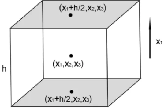
uiujwhere the bar indicates the mean taken over many cycles. The Reynolds stress, representing mean momentum flux, is a force per unit area directed in the xj-direction.

InFig. B.7, the x1-component of the per unit volume associated with the component

ρ

uiu1of the stress on the small fluid box with dimension h centered at (x1

,

x2

,

x3) is the difference between the forces on the shaded sides, or

1 h3

(−

h 2

_ρ

_u iuj

|

(x1+h/2,x2,x3)

+

h 2

_ρ

_u iuj

|

(x1−h/2,x2,x3)

).

(B.1)

Fig. B.7. Element of fluid acted upon by Reynolds stress.

Letting h

→

0, the force per unit volume for this component of the stress is

−

∂/∂

x1

(ρ

uiu1

)

; the total component force is found by summing over i. More generally, the force driving the mean streaming motion is F where

Fj

= −

−

i

∂/∂

xj

(ρ

uiuj

)

(B.2)

which is non-zero if there is some mechanism for attenuation of the sound wave. Without attenuation the gradient is zero and there is no mean forcing. We note that(B.2)is equivalent to

F

= −

ρ(

u

· ∇

u

+

u

∇ ·

u

)

(B.3)

used by Nyborg [78].

Two mechanisms for sound attenuation give rise to two primary forms of acoustic streaming: quartz wind and boundary induced streaming. With quartz wind the attenuation is a result of shear stresses in the body of the fluid. This effect can be observed in the laboratory when a quartz crystal is electrically excited producing strong ultrasonic beams off its faces into the surrounding air producing turbulent jets with velocities on the order of 10 cm

/

s. The quartz wind requires high acoustic power and high frequency for significant streaming velocities.

In boundary induced streaming the attenuation occurs in the layer of fluid (the Stokes layer) just outside a solid wall. Due to the strong shear stresses within this layer, attenuation is much greater and significant streaming occurs at relatively lower frequencies and powers. Boundary induced streaming is the principle behind the common science museum device known as a Kundt’s tube. A standing acoustic wave is established within a hollow tube containing fine dust. The dust accumulates at the antinodes of the standing wave, allowing the relationship between the frequency, wavelength, and sound speed to be established.

Appendix C. Progressive acoustic wave

We now show that a progressive acoustic wave transverse to a solid boundary leads to a steady streaming velocity in the direction of the wave, just outside the Stokes layer. The streaming is a result of the relative motion of the fluid and the boundary and streaming can result from either sound waves in the fluid or oscillations of the boundary. We use Lighthill’s formulation to compute the streaming velocity associated with a traveling acoustic wave directed in the

+

x-direction in a fluid in the region z

>

0 bounded by a solid wall at z

=

0. Let u and

v

be the x and y components of the fluid velocity. We assume the y component of the velocity is zero.

Suppose the amplitude of the traveling wave in the body of the fluid far from the wall is given by the real part12_of

U exp

(

i

(

nx

+

ω

t

)).

(C.1)

Momentum in the fluid diffuses with diffusivity

ν = µ/ρ

and the effect of the no-slip condition at the wall on the otherwise oscillating fluid diffuses according to e−z√iω/ν_{. Justification of this statement can be found in [31, section 2.7].} The x component of the fluid velocity is thus

u

=

U exp

(

i

(

nx

+

ω

t

))(

1

−

e−z

√

iω/ν

_).

_(C.2)

The Stokes layer is that region adjacent to the wall where the flow is rotational. InFig. C.8the real and imaginary parts of 1

−

exp

(−

z

√

i

ν/ω)

are plotted. For z

>

5

√

ν/ω

the effects of the boundary become insignificant and the flow is essentially irrotational. For this reason the Stokes layer thickness is taken to be, by convention,

Stokes layer

∼

5



ν/ω.

(C.3)

1 0 1 2 3 4 5 0.8 0.6 0.4 0.2

Fig. C.8. Estimate of the Stokes layer.

The z component of the velocity within the Stokes layer, required by the equation of continuity or incompressibility, is then

v =

inU



−

z

+

(

1

−

e−z √ iω/ν

₎



ν

i

ω



.

(C.4)

The force due to Reynolds stress(B.2)in the direction of x is

Fx

= −

∂(ρ

u2

)/∂

x

−

∂(ρ

u

v)/∂

z

.

(C.5)

The first term on the right side of this equation represents the rate of increase of x-momentum (per unit volume). In the present case of a traveling wave u2is independent of x and this term contributes no forcing.

Steady streaming with velocity uLat the edge of the boundary layer in the x-direction results from Fx

−

Fxinvwhere Fxinvis the inviscid part of Fxthat leads to no net streaming. Within the Stokes boundary layer the only significant force opposing

Fx

−

Fxinvis due to viscous stress. The steepest gradient of the viscous stress is in the z-direction so

µ

1u is dominated by the term

µ∂

2

₍

_u

_)∂

_z2_{and the mean streaming velocity at the edge of the boundary layer satisfies}

Fx

−

Fxinv

+

µ∂

2

₍

_u

_)∂

_z2

₌

₀

_,

_(C.6)

which can be integrated to obtain the streaming velocity just outside the boundary layer,

uL

= −

5 4n

ω

U

2

_.

_(C.7)

We remark that for a standing wave in a fluid, given by the real part of u

=

U

(

x

)

eiωt_{, one recovers the classical Rayleigh’s} law of streaming (see [31])

UL

= −

3

/(

4

ω)

U

(

x

)

U′

(

x

).

(C.8)

In this case both terms of(C.5)are non-zero with the first contributing

−

(

4

ω)

−1_U

₍

_x

₎

_U′

₍

_x

₎

_{and the second contributing}

−

(

2

ω)

−1U

(

x

)

U′

(

x

)

. References

[1] R.M. Moroney, R.M. White, R.T. Howe, Microtransport induced by ultrasonic Lamb waves, Appl. Phys. Lett. 59 (7) (1991) 774–776.

[2] T. Frommelt, M. Kostur, M. Wenzel-Schfer, P. Talkner, P. Hanggi, A. Wixforth, Microfluidic mixing via acoustically driven chaotic advection, Phys. Rev. Lett. 100 (3) (2008) 034502.

[3] B.R. Lutz, J. Chen, D.T. Schwartz, Microfluidics without microfabrication, Proc. Natl. Acad. Sci. 100 (8) (2003) 4395–4398.

[4] P. Marmottant, S. Hilgenfeldt, A bubble-driven microfluidic transport element for bioengineering, Proc. Natl. Acad. Sci. 101 (26) (2004) 9523–9527. [5] A. Wixforth, C. Strobl, C. Gauer, A. Toegl, J. Scriba, Z.v. Guttenberg, Acoustic manipulation of small droplets, Anal. Bioanal. Chem. 379 (2004) 982–991. [6] F. Caicci, P. Burighel, L. Manni, Hair cells in an ascidian (Tunicata) and their evolution in chordates, Hear. Res. 231 (1-2) (2007) 63–72.

[7] Y. Li, Z. Liu, P. Shi, J. Zhang, The hearing gene Prestin unites echolocating bats and whales, Curr. Biol. 20 (2) (2010) R55–R56.

[8] R.D. Rabbitt, H.E. Ayliffe, D. Christensen, K. Pamarthy, C. Durney, S. Clifford, W.E. Brownell, Evidence of piezoelectric resonance in isolated outer hair cells, Biophys J. 88 (3) (2005) 2257–2265.

[9] R. Feynman, There’s plenty of room at the bottom, Eng. Sci. 23 (5) (1960) 22–36.http://www.its.caltech.edu/~feynman/plenty.html. [10] J. Lighthill, Acoustic streaming in the ear itself, J. Fluid Mech. 239 (1992) 551–606.

[11] J. McCarren, Microscopic, genetic, and biochemical characterization of non-flagellar swimming motility in marine cyanobacteria, Ph.D. Thesis. Scripps Institution of Oceanography, Univ. of California, San Diego. download fromhttp://openwetware.org/wiki/Jay_McCarren, 2005.

[12] B. Brahamsha, Non-flagellar swimming in marine Synechococcus, J. Mol. Microbiol. Biotechnol. 1 (1999) 59–62. [13] K.F. Jarrell, M.J. McBride, The surprisingly diverse ways that prokaryotes move, Nat. Rev. Microbiol. 6 (6) (2008) 466–476.

[14] J. Koiller, K.M. Ehlers, F. Chalub, Acoustic streaming, the small invention of cyanobacteria? Arbor (CSIC), The Mathematics of Darwin special volume (in press).

[15] E.M. Purcell, Life at low Reynolds number, American J. Phys. 45 (1977) 3–11.

[16] K.M. Ehlers, A.D.T. Samuel, H.C. Berg, R. Montgomery, Do cyanobacteria swim using traveling surface waves?, Proc. Natl. Acad. Sci. USA 93 (1996) 8340–8343.