ACOUSTIC TOMOGRAPHY CONCEPT
S.M. JESUS AND C. SOARES
SiPLAB-FCT, University of Algarve, Campus de Gambelas, PT-8000 Faro, Portugal E-mail: \sjesus,csoaresi@ualg.pt
J. ONOFRE
Instituto Hidrogr´afico, Rua das Trinas 49, PT-1000 Lisboa, Portugal E-mail: mesquita.onofre@hidrografico.pt
E. COELHO
SACLANT Undersea Research Centre, Viale San Bartolomeo 400, 19138 La Spezia, Italy E-mail: coelho@saclantc.nato.int
P. PICCO
ENEA, Marine Environment Research Centre P.O. Box 224, 19100 La Spezia, Italy. E-mail: picco@estosf.santateresa.enea.it
Acoustic focalization is a well known concept that aims at estimating source location through the adjustment of multiple environmental parameters. This paper uses the same concept for inverting water column sound speed in a blind fashion, where both source location and source emitted waveform are not known at the receiver - that is Blind Ocean Acoustic Tomography (BOAT). The results obtained with BOAT, using ship noise data received on a vertical line array in a shallow water area off the coast of Portugal, show that it is indeed possible to obtain reliable joint estimates of source location and water column sound speed. During that process, it was shown that source range and depth, and Bartlett power, where good indicators of the degree of focus of the model being used.
1 Introduction
A consistent idea behind ocean acoustic tomography is that source and receiver relative positions, as well as source emitted signal characteristics, should be known to a high degree of precision. Deviations from this assumption generally have a direct impact in the inversion result. From a different perspective, Collins et al.>dH, suggested that source localization could be greatly facilitated by including additional (known) parameters into the search process in order to allow a better fit of the replica model - that is a technique known as acoustic focalization. The same concept has been readily used for generic parameter estimation in>1H, for geoacoustic inversion in >n, ;H and for source localization in [5–7].
A rather different concept has been proposed by Jesus et al.>MH, that attempts toes-timate channel propagation physical characteristics together with source properties. By
433
N.G. Pace and F.B. Jensen (eds.), Impact of Littoral Environmental Variability on Acoustic Predictions and Sonar Performance, 433-440.
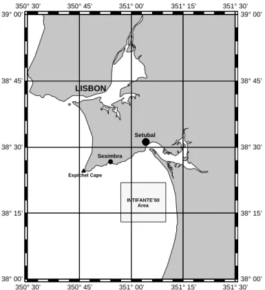
source properties, it is meant that the source position as well as the source emitted wave-form are unknown - this is Blind Ocean Acoustic Tomography (BOAT). Technically, BOAT has little difference from acoustic focalization, apart from the fact that the search space is enlarged to include truelly unkwown geometric, geoacoustic and water column parameters and that source characteristics are also unknown. There are great risks asso-ciated with such a global inversion procedure, one of which is that the final result may represent an “equivalent acoustic model” that may be far different from the true envi-ronment being sought. This is mainly due to the dramatic increase of the search space dimension and consequently an increase of the number of local maxima of the acoustic based objetive function. It was shown in [8], using active source data, that it is indeed possible to use source location parameters and the Bartlett power as indicators of the de-gree of “focus” of the environmental model, thus providing reliable water column sound speed estimates, when compared with independent recorded data. This paper pushes even further the concept of unknown source waveform by using acoustic ship noise, instead of deterministic high power source signals, to invert the environmental characteristics of a mildly range-dependent 3.3 km long track over a time interval of 1.5 h. In that regard it extends the preliminary results shown in [9] in the same data set, where a single time slot (2 s duration) at 1 km range and over a range-independent track was successfully inverted. 350° 30’ 350° 30’ 350° 45’ 350° 45’ 351° 00’ 351° 00’ 351° 15’ 351° 15’ 351° 30’ 351° 30’ 38° 00’ 38° 00’ 38° 15’ 38° 15’ 38° 30’ 38° 30’ 38° 45’ 38° 45’ 39° 00’ 39° 00’ INTIFANTE’00 Area LISBON Sesimbra Setubal Espichel Cape
2 The INTIFANTE’00 sea trial and the baseline model
The INTIFANTE’00 sea trial took place during October 2000, near the town of Set´ubal, approximately 50 km south from Lisbon, in Portugal (see Fig. 1). An overall description of the sea trial can be found in [10], whereas in this paper the interest will be focused only on Event 6, during which the signals received at the 16-hydrophone vertical line array (VLA) consisted on the noise radiated by the research vessel NRP D. Carlos I, cruising over a mildly range-dependent area up to 3.3 km range from the VLA. The NRP D. Carlos I is a 68 m overall length hydrographic ship with a gross displacement of 2800 tons. Her propulsion is obtained from a double helical diesel-electric engine with a total shaft power of 800 HP, attaining a maximum speed of 11 kn. It should be noted that NRP D. Carlos I was originally built for acoustic surveying so she is supposed to be a rather quiet ship. During Event 6, NRP D. Carlos I performed a triple bow shaped pattern at approximate ranges of 1.2, 2.2 and 3.3 km from the VLA as shown in Fig. 2. A detailed
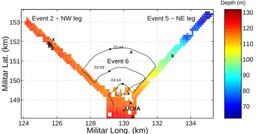
Depth (m) 70 80 90 100 110 120 130 124 126 128 130 132 134 149 150 151 152 153 x Event 5 − NE leg x x x ULVA Militar Long. (km) 02:14 02:44 03:14 Event 6 02:59 x x x x x x x Event 2 − NW leg Militar Lat. (km)
Figure 2. INTIFANTE’00 sea trial Event 6 and site bathymetry. XBT casts locations are marked with X and ULVA denotes the VLA location.
bathymetry of the area was not available, but approximate bathymetric profiles were made along both the NW and the NE tracks, as shown on Fig. 2. Therefore acoustic propagation between the ship and the VLA is assumed to be slightly downslope range-dependent to the NE, and progressively becoming range-independent, at 120 m water depth, to the NW. The maximum range-dependence is obtained for the 3.5 km range bow, with a maximum water depth difference of 20 m at the NE track. A number of XBT casts were made during the sea trial at various times and locations as marked by the X signs on Fig. 2.
Ship’s speed and heading, as obtained from GPS, is shown in Fig. 3, plots (a) and (b) respectively. It can be seen that mean ship speed was about 9 kn with several abrupt drops to 7 kn during the ship sharp turns along the triple bow trajectory.
291.090 291.1 291.11 291.12 291.13 291.14 291.15 291.16 2 4 6 8 10 12 14 Ship speed (kn) (a) 291.090 291.1 291.11 291.12 291.13 291.14 291.15 291.16 100 200 300 400 Bearing (deg) Julian date (b)
Figure 3. Event 6: GPS measured ship speed (a) and ship heading (b).
2.1 The Baseline Model
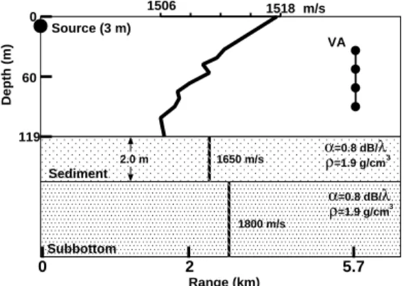
An important step towards a successful data inversion relies on the choice of a suitable environmental model. There was no extensive oceanographic or geoacoustic survey con-cerning the area of Event 6, and therefore, as in previous work [8], the same generic assumptions based on archival data were adopted, giving rise to the baseline model pic-tured in Fig. 4. Geoacoustic characteristics were empirically drawn from geological tables where the bottom was catalogued as “fine sand layer”. A two Empirical Orthog-onal Function (EOF) based model was used to represent the water column sound speed evolution through time and space, which coefficients are estimated together with the other
0 60 119 Depth (m) Range (km) Source (3 m) Sediment Subbottom 0 2 5.7 1506 1518 m/s 2.0 m 1650 m/s α =0.8 dB/λ ρ=1.9 g/cm3 α=0.8 dB/λ ρ=1.9 g/cm3 1800 m/s VA
Table 1. Focalization parameters and search intervals: EOF1 (α1), EOF2 (α2), source range (sr), source depth (sd), receiver depth (rd), VLA tilt (θ).
Symbol Unit Search int./Steps
α1 m/s -20 20 64 α2 m/s -20 20 64 sr km 0.5 3.5 64 sd m 1 10 32 rd m 85 95 32 θ rad -0.03 0.03 32
parameters. The EOF’s are deduced from XBT data taken at locations throughtout the experimental site, thus incorporating space and time variability into the EOF expansion (see X signs in Fig. 2). The searched parameters and their respective search intervals are listed in Table 1.
2.2 Ship Radiated Noise
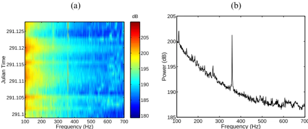
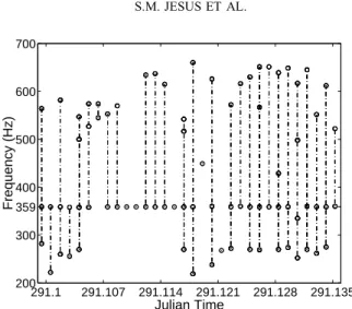
Acoustic signals were received on a moored vertical line array (VLA) with 16 hy-drophones, with its shallow and deep hydrophones positioned at nominal depths of 32 and 92 m, respectively. Array depth and tilt were recorded during the experiment. Figure 5 shows the signals received on hydrophone 8 (60 m depth), on panel (a) a time-frequency plot, and in panel (b) a mean power spectrum over the whole event. There are clearly a few characteristic frequencies emerging from the background noise between 250 and 260 and a strong single tone at 359 Hz. There is also a coloured noise spectra in the band 500 to 700 with however, a much lower power. As a preliminary analysis, a power spectrum estimator was run on a 8 s sliding time window throughout all the event duration and the maximum power frequency bins were automatically extracted. Figure 6 shows the selected frequency bins that were then used in the inversion procedure.
(a) (b) dB 180 185 190 195 200 205 Frequency (Hz) Julian Time 100 200 300 400 500 600 700 291.1 291.105 291.11 291.115 291.12 291.125 100 200 300 400 500 600 700 185 190 195 200 205 Frequency (Hz) Power (dB)
Figure 5. NRP D. Carlos I ship radiated noise received on hydrophone 8: time-frequency plot (a) and mean power spectrum (b).
291.1 291.107 291.114 291.121 291.128 291.135 200 300 359 400 500 600 700 Julian Time Frequency (Hz)
Figure 6. INTIFANTE’00 sea trial, event 6: selected frequency bins for inversion. 3 Inversion results
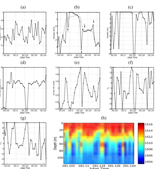
The inversion methodology was based on a three step procedure: i) preliminary search of the outstanding frequencies in a given time slot, ii) parameter focalization, based on an incoherent broadband Bartlett processor, a C-SNAP forward acoustic model and a GA based optimization and iii) inversion result validation based on model fitness and coherent source range and depth estimates through time. The inversion results are shown in Fig. 7, from (a) to (g) are individual parameter estimates while plot (h) shows the water column sound speed reconstruction based on the EOF linear combination based on parameter estimates (f) and (g).
At first glance the results are poor: Bartlett power is low, always below 0.8; source range and depth, which are leading parameters, show highly incoherent values; and finally the reconstructed sound speed is too variable for such a small time interval (less than 1 h 30 min). Looking more in detail, and comparing plot (a) of Fig. 3 with plot of Fig. 7 the following conclusions can be drawn:
1. For time≤ 291.101 no results can be obtained since the ship is at low speed, Bartlett power is low and parameter estimates are messy.
2. For 291.101≤ time ≤ 291.107, ship speed increases steeply to 9 kn, while heading away from the VLA. Range variation is about 4.6 m/s which, may cause a violation of the stationary assumption during the averaging time. Estimates are also messy during this period.
3. At time = 291.108, the ship makes a sharp turn (slowing down to 7 kn) and initiates the first bow at an approximate range of 3.2 km and at constant speed of 9 kn. At this point the estimation peaks up for a time period between 291.109 to 291.130, i.e. approximately 30 min with a unique exception at 291.119 where there is an estimation loss. That estimation loss curiously corresponds to another sharp turn when the ship heads towards the array between the 3.2 km and the 2.2 km bow. With that exception it can be noticed that range estimates generally coincide to the GPS measurements. There is a slight range error at the begining of the 3.3 km bow
(a) (b) (c) 291.102 291.11 291.118 291.126 291.134 0 0.2 0.4 0.6 0.8 1 Julian Time Bartlett Power 291.102 291.11 291.118 291.126 291.134 0.5 1 1.5 2 2.5 3 3.5 Julian Time Range (km) 291.102 291.11 291.118 291.126 291.134 1 2 3 4 5 6 7 8 9 10 Julian Time Depth (m) (d) (e) (f) 291.102 291.11 291.118 291.126 291.134 85 90 95 Julian Time Sensordepth (m) 291.102 291.11 291.118 291.126 291.134 −0.03 −0.02 −0.01 0 0.01 0.02 0.03 Julian Time
Array tilt (rad)
291.102 291.11 291.118 291.126 291.134 −20 −15 −10 −5 0 5 10 15 20 Julian Time α1 (g) (h) 291.102 291.11 291.118 291.126 291.134 −20 −15 −10 −5 0 5 10 15 20 Julian Time α2 1504 1506 1508 1510 1512 1514 1516 291.102 291.11 291.118 291.126 291.134 0 20 40 60 80 100 Julian Time Depth (m)
Figure 7. Focalization results for Event 6: Bartlett power (a), source range and GPS measured range (dashline) - arrows indicate sharp ship turns (b), source depth (c), receiver depth (d), VLA tilt (e), EOF coefficient 1 (f), EOF coefficient 2 (g) and reconstructed sound speed (h).
(t=291.11) possibly due to range-dependency mismatch which is the strongest at this point (20 m depth difference between source and array position). Sensor depth and array tilt show credible values with an interesting behaviour of the later that varies from -0.03 to +0.03 almost linearly and possibly due to a change of the source view angle due to the 45 degree turn along the bow shaped track.
4. At time 291.131 there is another sharp turn towards the array with a speed drop and another estimation loss.
5. For the remaining few minutes the parameter estimation resumes during the closest range bow at 1.2 km from the VLA.
As a final comment, it can be added that the reconstructed sound speed suffers from the consecutive losses of estimation that fully coincide with the estimation losses verified in the other curves and are directly related to ship maneuvering and speed drops.
4 Conclusion
Ocean tomography with sources of opportunity has been a longely sought dream for acoustic oceanographers. This paper presents a preliminary result obtained in a shallow water area off the continental coast of Portugal during the INTIFANTE’00 sea trial, that proves the feasibility of the BOAT concept using ship radiated noise as input signal for tomographic inversion. Although the duration of the acoustic data was manifestly too short for a complete oceanographic validation, it was clearly seen that the estimates could be validated by the conjugation of the Bartlett power and obtaining coherent source range and depth values. Using this three parameters it becomes clear when the environment is “in focus” and when it is “out of focus”. The computational effort was reasonabe due to an efficient carry on of model information from one time sample to the next in order to allow a simplified search.
Acknowledgements
This work was supported by FCT, Portugal, under projects INTIMATE (2/2.1/MAR/1698/95) and ATOMS (PDCTM/P/MAR/15296/1999). The authors are also in debt to the crew of NRP D. Carlos I of IH, that made the sea trial successful.
References
1. Collins, M.D. and Kuperman, W.A., Focalization: Environmental focusing and source local-ization, J. Acoust. Soc. Am. 90(3), 1410–1422 (1991).
2. Gerstoft, P. and Gingras, D., Parameter estimation using multi-frequency range-dependent acoustic data in shallow water, J. Acoust. Soc. Am. 99(5), 2839–2850 (1996).
3. Gerstoft, P., Inversion of seismoacoustic data using genetic algorithms and a posteriori prob-ability distributions, J. Acoust. Soc. Am. 95(2), 770–782 (1994).
4. Hermand, J.-P. and Gerstoft, P., Inversion of broad-band multitone acoustic data from the YELLOW SHARK summer experiments, IEEE J. Oceanic Eng. 21(4), 324–364 (1996). 5. Soares, C., Waldhorst, A. and Jesus S., Matched field processing: Environmental focusing and source tracking with application to the North Elba data set. In Proc. MTS/IEEE
Oceans’99, Seattle, Washington, USA (1999), pp. 1598–1602.
6. Soares, C.J., Siderius, M. and Jesus, S.M., Matched-field source localization in the Strait of Sicily, J. Acoust. Soc. Am. (in press 2002).
7. Soares, C., Siderius, M. and Jesus, S., High frequency source localization in the Strait of Sicily. In Proc. MTS/IEEE Oceans 2001, Honolulu, Hawaii, USA (2001).
8. Jesus, S.M., Coares, C., Onofre, J. and Picco P., Blind ocean acoustic tomography: Exper-imental results on the INTIFANTE’00 data set. In Proc. 6th European Conference on
Underwater Acoustics, Gdansk, Poland (June 2002).
9. De Marinis, E., Gasparini, O., Picco, P., Jesus, S., Crise, A. and Salon, S., Passive ocean acoustic tomography: theory and experiment. In Proc. 6th European Conference on
Un-derwater Acoustics, Gdansk, Poland (June 2002).
10. Jesus, S.M, Coelho, E., Onofre, J., Picco, P., Soares, C. and Lopes, C., The INTIFANTE’00 sea trial: preliminary source localization and ocean tomography data analysis. In Proc.