Civil and criminal identification with Bayesian networks

(1)

CIVIL AND CRIMINAL IDENTIFICATION

WITH BAYESIAN NETWORKS

ANDRADE Marina, (PT), FERREIRA Manuel Alberto M., (PT)

Abstract. The use of DNA evidence in problems of civil and criminal identification is becoming greater and greater. Being necessary to evaluate the weight of that evidence one of the most powerful tools to help in it is the Bayesian networks. This is exemplified with the presentation of a civil identification problem and of a criminal identification problem in this work.

Key words: Bayesian networks, DNA database profiles, civil and criminal identification problems.

Mathematics Subject Classification: 62C10.

1 Introduction

In this work it is intended to exemplify how to apply Bayesian networks in civil and criminal identification problems. The first objective is to give a methodology, with the appropriate tools, to use in a correct way a DNA profiles database in the problem of civil identification when there is a partial match between the genetic characteristic of an individual whose body was found, one volunteer who claimed a family member disappearance and one sample belonging to the DNA database.

In section 2 the civil identification case to be studied is presented and discussed. The Bayesian network, that allows the efficient probabilities computation, determinant to evaluate the hypothesis in comparison, is presented. In section 3, real examples clarifying the application are exhibited. And in section 4 a brief discussion is outlined related with this objective.

The second objective is to illustrate the use of biological information in crime scene identification problems, example of a criminal identification problem. In section 5 a crime scene, the correspondent evidence, E, and the hypotheses to be considered are presented. In section 6 the Bayesian network built expressly to perform the calculations is shown. And in section 7 the numerical results will be seen. Finally in section 8 a brief discussion, related with this second objective is presented.

(2)

Aplimat – Journal of Applied Mathematics

174 volume 5 (2012), number 3

General conclusions and references are presented at the end of the paper.

2 The Civil Identification Problem

Frequent examples of civil identification problems are the case of a body identification, jointly with information of a missing person belonging to a known family, or the identification of more than one body resultant of a disaster or an attempt. And even immigration cases in which it is important to establish family relations.

The establishment and use of DNA database files for a great number of European countries was an incentive to study the mentioned problems and the use of these database files for identification, (Corte-Real, 2004), (Martin, 2004) and (Andrade and Ferreira, 2009a, 2010). In this context it may be useful when unidentified corpses appear and may be identified by comparison of their DNA profiles with family volunteer's profiles.

The Portuguese law nº 5/2008 establishes the principles for creating and maintaining a database of DNA profiles for identification purposes, and regulates the collection, processing and conservation of samples of human cells, their analysis and collection of DNA profiles, the methodology for comparison of DNA profiles taken from the samples, and the processing and storage of information in a computer file1.

So the database is, in general terms, composed of a file containing information of samples from convicted offenders with 3 years of imprisonment or more - ; a file containing the information of samples of volunteers - ; a file containing information on the “problem samples” or “reference samples” from corpses, or parts of corpses, or things in places where the authorities collect samples - .

It matters to study civil identification problems, mainly if there is a partial match between the genetic characteristic of an individual whose body was found and one volunteer who claimed a family member disappearance and one sample in the database file .

2.1 The Case of Partial Match with the Volunteer and one

When there is an individual claiming for a disappeared person who gives his/her genetic characteristic, , to be compared with the genetic characteristic of a body found, the first action to do is to check if there is a match between the genetic characteristic of the individual whose body was found, , and any sample of the DNA file, - sample, which is named “problem samples”. If there is a partial match between the genetic profile of the individual whose body was found and one sample in the file , the evidence now is , – , .

Then it follows the establishment of the hypotheses of interest: the identification hypothesis versus the non identification hypothesis :

: It is possible to reach an identification of the individual whose body was found. vs

1_{The implementation of this process is not going very well. In the moment the number of samples in database is not} significant.

(3)

volume 5 (2012), number 3 175

: It is not possible to reach an identification of the individual whose body was found.

After checking the possibility of a partial match between the profile of the individual whose body was found, , the sample in the file , - sample, and the volunteer, , two different comparisons are made in order to obtain a measure either of the possible genetic relation between the individual whose body was found with the - sample (bf_match_gs?), or of the possible genetic relation between the individual whose body was found and the volunteer (bf_match_vol?). The possible answers are: yes or no.

So the resulting states are:

 A (yes, no) - defines the possibility of genetic relationship between the individual whose body was found and the - sample but not the volunteer;

 B (no, yes) - defines the possibility of genetic relationship between the individual whose body was found and the volunteer but not the - sample;

 C (yes, yes) - defines the possibility of genetic relationship between the individual whose body was found and both the volunteer and the - sample;

 D (no, no) - defines the possibility of genetic relationship between the individual whose body was found neither with the volunteer nor with the - sample;

A, B define the identification hypothesis, , and C, D define the non identification hypothesis,

. B is a particular case: the simple problem studied in (Andrade and Ferreira, 2009a). Each of

the four possible states probabilities provides a measure for each event, and the four are pairwise incompatible.

Following the probabilities computation it is important to compare state D versus A, B, C; i.e., to evaluate the event “the individual whose body was found is not genetically related either with the - sample or the volunteer”. This comparison intends to evaluate the situation “the genetic information of the individual whose body was found is not compatible with the other genetic information available” and “the genetic information of the individual whose body was found is compatible with at least one of the remaining genetic information”.

If D is accepted the process ends. And the body genetic information joins the file in the database. If D is discarded then it is necessary to perform a comparison between A, B and C events. If C is accepted the process ends and police intelligence investigations must be done. If C is discarded, finally A and B must be compared. If A is accepted the individual whose body was found is related with the - sample. If B is accepted the conclusion is that the individual whose body was found is a volunteer relative.

3 The Bayesian Network for the Civil Identification Problem

The comparisons described above are performed through the respective probabilities events ratios: the likelihood ratios, (Ferreira and Andrade, 2009). The hypothesis with the greatest probability is the accepted one. Thus the probabilities associated to the states A, B, C and D must be computed. In

(4)

176 volume 5 (2012), number 3

order to do so a lot of intermediary conditional probabilities computation, that are impossible to do with algebraic manipulations, must be done.

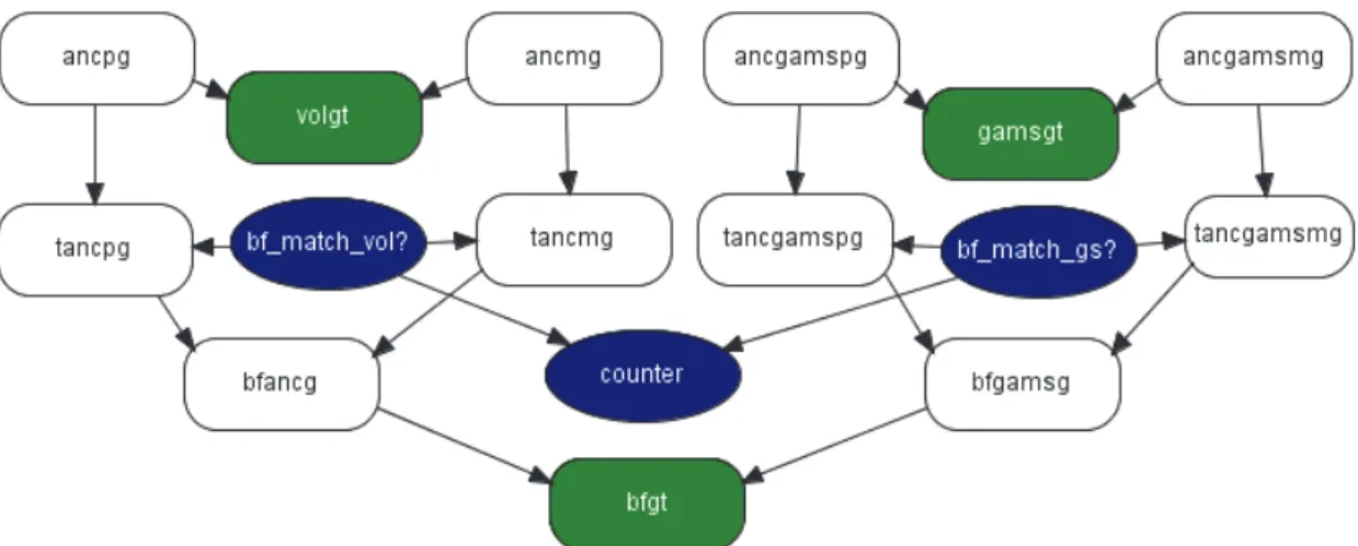
To overcome this situation those probabilities will be computed using the Bayesian network, see (Andrade and Ferreira, 2009) and (Andrade et al., 2010), in the Figure 12.

Figure 1: Network for civil identification with one volunteer and one

The nodes ancpg, ancmg, ancgampg and ancgammg are of class founder: a network with only one node which states are the alleles in the problem where the respective frequencies in the population are specified, and represent the volunteer's ancient paternal and maternal inheritance.

The nodes volgt, gamsgt and bfgt are of class genotype: the volunteer, the - sample and the body found genotypes.

Nodes tancmg, tancpg, tancgamspg and tancgamsmg specify whether the correspondent allele is or is not the same as the volunteer and the same as the - sample.

If bf_match_vol? is true then the volunteer's allele will be identical with the body found allele, otherwise the allele is randomly chosen in the population and if bf_match_gs? is true then the - sample's allele will be identical with the body found allele, otherwise the allele is randomly chosen in the population.

The nodes bfancg and bfgamsg define the Mendel inheritance in which the allele of the individual whose body was found is chosen at random from the ancient's paternal and maternal gene.

Node counter counts the number of true states of the preceding nodes, accounting the results for the A, B, C, D possible events.

3.1 Examples

To exemplify the described methodology, in Table 1 the allele frequencies, real ones, for some genetic markers and, for each marker, possible evidence profiles for the body found , the - sample and the volunteer are presented.

(5)

Aplimat – Journal of Applied Mathematics volume 5 (2012), number 3 177 Marker Allele Frequencies , – , D21S11 . _{29,30 , 28,30 , 29,31.2} 0.1647 0.2136 0.2437 0.1138 F13A1 _{6,7 , 7,8 , 5,6} 0.1985 0.2890 0.3377 0.0112 TH01 . _{7,9 , 9,9.3 , 6,7} 0.2044 0.1696 0.1984 0.2748 TPOX _{8,11 , 8,10 , 9,11} 0.5053 0.0974 0.0647 0.2893 VWA31 _{16,17 , 15,17 , 16,18} 0.1216 0.2300 0.2649 0.1859

Table 1: Allele frequencies and genetic profiles.

In Table 2 the state probabilities, the node counter states, see Figure 1, are presented.

States D21S11 F13A1 TH01 TPOX VWA31

A 0.5322 0.3296 0.4987 0.2661 0.4548 B 0.1296 0.2226 0.1978 0.2688 0.2251 C D 0.2274 0.1108 0.1904 0.2574 0.1692 0.1343 0.1539 0.3112 0.2092 0.1109

Table 2: State probabilities.

And in Table 3 the decisions, consequence of the procedures proposed in section 2.1, are presented for each example evidence profile.

Evidence Profiles Decision 29,30 , 28,30 , 29,31.2 Police intelligence investigations must be done 6,7 , 7,8 , 5,6 The individual whose body was found is a volunteer relative 7,9 , 9,9.3 , 6,7 Police intelligence investigations must be done 8,11 , 8,10 , 9,11 The individual whose body was found is a volunteer relative 16,17 , 15,17 , 16,18 Police intelligence investigations must be done Table 3: Decisions for each evidence profile.

4 First Discussion

Using the Bayesian network built expressly for civil identification problem, in which there is a partial match between an individual whose body was found, a volunteer who claimed a relative disappearance supplying his/her own genetic information and a DNA database file sample existent, it is possible to perform the sequence of three hypothesis tests described above. Thus it is possible

(6)

178 volume 5 (2012), number 3

to decide first if an identification is possible or not; second if an effective identification is possible or not; third to make the identification. So with a procedure technically simple, it is possible to make an adequate and correct use of a DNA database.

As the examples illustrate, the procedure leads almost surely to a decision: whether it is to close the case identifying the individual, or concluding that it is not possible any identification, or to go on with the police investigations.

5 Crime Scene Investigation

A crime has been committed. Two persons, V1 and V2, were murdered. One mixture trace was found. S1 and S2 are potential suspects. S1 and S2 DNA profiles were measured and considered to be compatible with the mixture trace.

Being possible that a fight occurred during the assault, producing some material, it is acceptable that the individuals who perpetrated the crime could have left some of their material in the trace. To analyse the crime scene, in this section, it will be presented the evidence, E, and the hypotheses to be considered.

To summarize the evidence it is presented in Table 4 the DNA profiles of the victims’ and the suspect’s, V1, V2, S1, S2, and the trace found at the crime scene, E.

V1 V2 S1 S2 E

TH01 9,9.3 9,9.3 7,8 6,9 6,7,8,9,9.3

F13A1 5,7 5,6 3.2,5 6,7 3.2,5,6,7

FGA 22,26 22,23 24,24 19,24 19,22,23, 24,26

Table 4: Two victim’s and two suspect’s DNA profiles and evidence. In Table 5 the allele frequencies, for each marker found in the trace, are presented.

p6 p7 p8 p9 p9.3 TH01 0.2044 0.1696 0.1386 0.1984 0.2748 p3.2 p5 p6 p7 F13A1 0.0806 0.1985 0.2890 0.3377 p19 p22 p23 p24 p26 FGA 0.0684 0.1740 0.1606 0.1325 0.0321

Table 5: Allele frequencies.

The allele frequencies in Table 5 are the Portuguese population frequencies collected in the database “The Distribution of Human DNA-PCR Polymorphisms”, since the mentioned case is supposed to have occurred in Portugal.

The crime trace can contain DNA from up to four unknown contributors, in addition to the victims and/or the suspects.

(7)

volume 5 (2012), number 3 179

If the DNA of Si with i = 1, 2 is presented in the trace this will place him/her at the crime scene and

consequently as one of the possible perpetrators.

The court has to determine if each suspect is or is not guilty. The hypotheses to be evaluated are: H1: S1 is a contributor to the trace but S2 is not, given the evidence.

H2: S2 is a contributor to the trace but S1 is not, given the evidence. H3: S1 and S2 are both contributors to the trace, given the evidence. H4: Neither S1 nor S2 are contributors to the trace, given the evidence.

The respective events probabilities are called p10, p02, p12, p00, where 0 mentions the absence of the respective, in order, individual DNA in the trace. So:

If p00 > p10 + p02 + p12 the two suspects are acquitted. If not it must be seen if p12 > p10 + p02 case at which the two suspects are both placed at the crime scene. If not p10 must be compared with p02. If p10 > p02 the evidence favours the presence of S1 at the crime scene and the acquaintance of S2. The contrary happens when p02 > p10.

6 Marker Bayesian Network

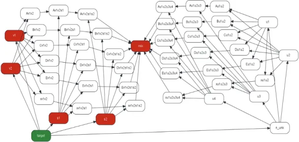
The probabilities referred above are very hard to compute algebraically, demanding a great use of Bayes’ Law because of the number of the dependencies to be considered. So they will be computed using the Bayesian network of Figure 2.

Figure 2: Marker network

Nodes vi, i = 1, 2, sj, j = 1, 2 and uk,k = 1, 2, 3, 4, in Figure 2 are themselves Bayesian networks that

represent the genetic structure and inheritance of each individual - the victims, the suspects and the unknowns, respectively - and have all the same structure. The vi, i = 1, 2 and sj, j = 1, 2 are

represented in red colour meaning that the respective profiles are known and constitute data of the problem. The nodes in white, below the node mix, that represents the mixture and is also in red colour because it is comprised by known data (E), represent the relations in which the nodes in red may contribute to the mixture. The nodes in white, above the node mix, except the uk,k = 1, 2, 3, 4

(8)

180 volume 5 (2012), number 3

which the uk,k = 1, 2, 3, 4 may contribute to the mixture. Node target, in green colour, collects the

states and the respective probabilities.

As it is mandatory to consider the possible contribution of till four unknown individuals to the mixture, the number of admissible states jumps to 80, numbered from 0 - no one in the mixture - to 79 - the two victims, the two suspects and the four unknowns are all in the mixture. Of course these two states are unrealistic and there are other ones also unrealistic because are incompatible with the minimum number of contributors to the mixture, according to the evidence inserted. These unrealistic states are discarded by the network but have to be considered conceptually in its building.

Among the realistic states only a few ones are interesting to the problem: the corresponding to the hypotheses events defined above.

7 Numerical Results

For marker TH01, alleles 6, 7, 8, 9, 9.3 are considered, Table 4, and so they are represented in the Figure 1 Bayesian network by A, B, C, D, E, respectively. When considering marker F13A1, the alleles are 3.2, 5, 6, 7, corresponding to A, B, C, D. E is considered with 0 frequency. In marker FGA the alleles are 19, 22, 23, 24, 26 corresponding to A, B, C, D, E. In any case x accumulates the remaining frequencies of the non considered alleles for each marker.

The results obtained using Table 4 data together with Table 5 frequencies are in Table 6, where the values in line rescale are constituted by the ratios of the products of the values in the respective column3 by the total sum of the four products. The values in this line are the used ones in the tests described in section 5. p00 p12 p10 p02 TH01 0.0830 0.5029 0.2773 0.1367 F13A1 0.0986 0.4544 0.3279 0.1187 FGA 0.0378 0.4398 0.0820 0.4398 Rescale 0.0027 0.8709 0.0646 0.0618 Table 6: Results.

Following the procedure outlined in section 5 the conclusion is that both suspects are placed at the crime scene – note the great value of p12 = 0.8709. For TH01 and F13A1, alone, the conclusion is the same. But for FGA this does not happens. Note that, p12 = p02. This is justified by the fact that in marker FGA there are two rare alleles, p19 = 0.0684 and p26 = 0.0321, that are in consequence “good identifiers”. Each one is present in V1 and S2. Besides S1 is homozygote for this marker and this genotype may be hidden by S2’s genotype. In consequence it is natural that p12 and p02 are of the same magnitude.

To compute the interesting probabilities there must be considered the following states probabilities:

3_{It is possible to multiply the respective probabilities, for each marker, because it is assumed independence between} and across marker, i.e., linkage and Hardy-Weinberg Equilibrium [8].

(9)

Aplimat – Journal of Applied Mathematics volume 5 (2012), number 3 181 - p00: 1, 2, 3, 16, 17, 18, 19, 32, 33, 34, 35, 48, 49, 50, 51, 64, 65, 66 and 67, - p12: 12, 13, 14, 15, 28, 29, 30, 31, 44, 45, 46, 47, 60, 61, 62, 63, 76, 77, 78 and 79, - p10: 8, 9, 10, 11, 24, 25, 26, 27, 40, 41, 42, 43, 56, 57, 58, 59, 72, 73, 74 and 75, - p02: 4, 5, 6, 7, 20, 21, 22, 23, 36, 37, 38, 39, 52, 53, 54, 55, 68, 69, 70 and 71 from the output given by Hugin after the inserted evidence.

8 Second Discussion

Criminal identification problems are examples of situations, in which forensic approach, the DNA profiles study is usual. But the interpretation and evaluation of DNA evidences is not an easy task, see for instance, (Andrade and Ferreira, 2011) and (Lauritzen, 2003). Also the fact that in general they are posed in probabilistic terms leads to some confusion to the judges when they have to issue a decision. In this situation the Bayesian approach is maybe the most clear to explain the significance of the evidence, see (Ferreira and Andrade, 2009). And for it the use of Bayesian networks to compute the interesting probabilities is a natural option, as it was exemplified in this paper.

It is important to define which probabilities, among the possible ones to compute, interest to the problem. And in consequence to define, for each case, which hypotheses tests to implement. Of course they are Bayesian tests.

Note finally, as this example shows, that this methodology may conclude for the absolution of a suspect but not for the conviction. It only can place the suspect in the crime scene. Further work of the police must be made to conclude by the conviction or absolution.

9 General Conclusions

The use of networks transporting probabilities began with the geneticist Sewall Wright in the beginning of the 20th century (1921). (Dawid et al., 2002) describes this new approach to problems of the kind of the one described above. The construction and use of Bayesian networks to analyse problems in forensic identification inference, was initially done there, followed by (Evett et al., 2002), (Mortera, 2003) and (Mortera et al., 2003).

The civil identification problem presented obviously may occur in situations of catastrophes or accidents at which it is possible to have unidentified victims. The use of DNA evidence is quite recent in helping to solve this situations. It was shown in this work how the use of Bayesian networks is useful to evaluate that kind of evidence.

The analysis of a crime scene analogous to the considered in this work, but with two victims’ and one perpetrator and two mixture traces was presented in (Andrade and Ferreira, 2009, 2011b, 2011c). A problem dealing with a crime scene analogous to the one considered in this work may be seen at (Andrade and Ferreira, 2011a). Also was shown in this work how useful are the Bayesian networks in the evaluation of DNA evidence in problems of criminal identification.

(10)

182 volume 5 (2012), number 3

Acknowledgement

This work was financially supported by FCT through the Strategic Project PEst-OE/EGE/UI0315/2011.

References

ANDRADE, M.: A Estatística Bayesiana na Identificação Forense: Análise e avaliação de vestígios de DNA com redes Bayesianas. Phd Thesis, ISCTE, 2007.

ANDRADE, M.: A Note on Foundations of Probability. Journal of Mathematics and Technology, vol. 1 (1), pp 96-98, 2010.

ANDRADE, M. and FERREIRA, M. A. M.: Bayesian networks in forensic identification problems. Aplimat - Journal of Applied Mathematics, vol. 2 (3), pp. 13-30, 2009.

ANDRADE, M. and FERREIRA, M. A. M.: Civil identification problems with DNA databases using Bayesian networks. International Journal of Security-CSC Journals, vol 3 (4), pp 65-74, 2009a.

ANDRADE, M. and FERREIRA, M. A. M.: Civil identification problems with Bayesian networks using official DNA databases. Aplimat-Journal of Applied Mathematics, vol. 3 (3), pp 155-162, 2010.

ANDRADE, M. and FERREIRA, M. A. M.: Some considerations about forensic DNA evidences. International Journal of Academic Research, vol. 3, (1, Part I), pp 7-10, 2011.

ANDRADE, M. and FERREIRA, M. A. M.: Evidence evaluation in DNA mixture traces possibly resulting from two victims and two suspects. Portuguese Journal of Quantitative Methods, vol 2 (1), pp 99-103, 2011a

ANDRADE, M. and FERREIRA, M. A. M.: Crime scene investigation with probabilistic expert systems. International Journal of Academic Research, vol. 3 (3, Part I), pp 7-15, 2011b.

ANDRADE, M. and FERREIRA, M. A. M.: Crime scene investigation with two victims and a perpetrator. 4 th IISMES Conference, Dalian, P. R. China. 2011c. Forthcoming.

ANDRADE, M., FERREIRA, M. A. M., ABRANTES, D., PONTES, M. L. and PINHEIRO, M. F.: Object-oriented Bayesian Networks in the evaluation of paternities in less usual environments. Journal of Mathematics and Technology, vol. 1 (1), pp 161-164, 2010.

Corte-REAL, F.: Forensic DNA databases. Forensic Science International. 146s:s143-s144, 2004. DAWID, A. P., MORTERA, J., PASCALI, V. L. and BOXEL, D. W.: Probabilistic expert systems for forensic inference from genetic markers. Scandinavian Journal of Statistics vol. 29, pp 577-595, 2002.

EVETT, I. W., GILL, P. D., JACKSON, G., WHITAKER, J. and CHAMPOD, C.: Interpreting small quantities of DNA: the hierarchy of propositions and the use of Bayesain networks. Journal of Forensic Science, vol. 47, pp 520-539, 2002.

FERREIRA, M. A. M. and ANDRADE, M.: A note on Dawnie Wolfe Steadman, Bradley J. Adams, and Lyle W. Konigsberg, Statistical Basis for Positive Identification in Forensic Anthropology. American Journal of Physical Anthropology 131: 15-26 (2006). International Journal of Academic Research, vol. 1 (2), pp 23-26, 2009.

LAURITZEN, S. L.: Bayesian networks for forensic identification Problems. Tutorial 19th Conference on Uncertainty in Artificial Intelligence, Mexico, 2003.

MARTIN, P.: National DNA databases - practice and practability. A forum for discussion. In International Congress Series 1261, pp 1-8, 2004.

(11)

volume 5 (2012), number 3 183

MORTERA, J.: Analysis of DNA mixtures using probabilistic expert systems. In: P. J. Green, N. L. Hjort and S. Richardson (Eds.), Highly Structured Stochastic Systems. Oxford University Press, 2003.

MORTERA, J., DAWID, A. P. and LAURITZEN, S. L.: Probabilistic expert systems for DNA mixture profiling. Theoretical Population Biology, vol. 63, pp 191-205, 2003.

Current address

Marina Andrade, Professor Auxiliar

ISCTE – Lisbon University Institute UNIDE - IUL

Av. Das forças armadas 1649-026 Lisboa

Telefone: + 351 21 790 34 05 Fax: + 351 21 790 39 41

e-mail: [email protected]

Manuel Alberto M. Ferreira, Professor Catedrático

ISCTE – Lisbon University Institute UNIDE - IUL

Av. Das forças armadas 1649-026 Lisboa

TELEFONE: + 351 21 790 37 03 FAX: + 351 21 790 39 41

(12)