Estimating common sectoral cycles

JOURNALOF

Monetmv

___.._L__.. ____ -- _ -_- .-.- . _ _ AbWlrCl

Wc invcstipatc in this paper the degree of shorl-run and long-run comovcmcnt in I! S. szitoral output data by e:;timuting scctoral :r:n& and cycles. A thcorLtical model hascd on Long and Plosser ( 1983) i:, usrd to derive 3 reduced form for sectoral outputs from tirst principles. Cointclpr;ltion and common-cycle lcsts arc performed; sectoral output data seem to share ii rclativcly high nurntw of common trends und 3 relatively low nurthcr of common cycles. A special trcncl-cycle &composition of the data set is performed. and the results indicate P bury similar cyc1ic.d behavior :wrws scct,)rs and iery difletcnt beh:lvior for trends. In ;I var\;tncc dc~~m~pc~t~w .tn;d! \I*;. prominent w:ctors wch ;I* hl,wdactur- ing ;III~ Wholcdc Hclilll Tr;dc callihlt rclallvLlg imijortilnt tr;lnsrlory shr)ckb.

I. Introduction

C’ontcmporary business c)cIc WscilrCh li)Cllscs upon movements in iIggW&lle 1Nl~plJ~. (‘ompi~rkms Of sllllpk \IiJliStkiJl chilractcristics liIbCkd ‘SlyliZCd hCtS’

with clahoratc rigorous theoretical prcdi.*tions arc cailcd ‘calibration’ and form the central paradigm in this research programme initiated by Kydl:*r:J el..: Prescott (1982). In particular, the persistence of aggregate shocks is a central feature of such comparisons and one of the important developments was the discovery of theoretical models which could mimic this observed persistence.

This focus is, however. quite difl’crcnt from cithcr the data-intcnsivc analysis of the early NBER rcscarchcrs. as documented in Burns and Mitchell (1946), or the macroeconometrlc anal~scs of the sixties perhaps best cxcmplihcd by the Brookings MO&~, as described in Duescnberry cl 31. (1965). In these studies. statistical analysis ofcomovcmcnts bctwccn sectors and products rcceivcs care- ful attention, but theoretical modeihng plays a secondal.< role. Cycles are characterized by coordinate movements across sectors as well as persistence of shocks. The ability to identify cycles is greatly strengthened by the use of the additional information fclund in sectoral disaggrcgation.

Although the theoretical litciature on business cycles has advanced consider- ably in the last fifteen years. e.g.. Long and Plosser (1983), the empirical literature has not kept pact with it. One of the shortcomings is the lack of studies using sectorally disaggregated data. Notable exceptions are Long and Plosser (1987) and Pesaran et al. (1993). However, even these studies did not analyze the cicgrec of short- and long-run comovement present in the data. There is a good reason for such incomplclencss though. since only recently have the appropriate statistical tools been available to allow comovement comparisons.

The present paper dxdmincs jointly the degree of short- and long-run comovc- mcnt prcscnt m U.S. output scrics by using a newly do*d!:)oped multivariatc method called COI)II~IO~I tn*ntls cortl (YJIIII~IO)I c~~~~/e.s. The llrcthodology is described in Vahld aIld l!ng’: (19C!). following Engle and Kozicki (1933). It works under the assumption that the data contain unit-roots, therefore stochastic trends, c.g.. Stock and Watson (1988). Searching for common trends amounts to performing cointegration tests, which can be 1:lterpreted as long-run comovcmcnt tests. Thus, we build on the cointegration literature motivatf*d b) the work ofC;rangcr (19133. 1986) and En& and Grangcr (19x7). C’yclcs arc modcllcd ;I:, transitory but pcrsistcllt proccsscs which may bc ccmmon to several sectors. Such cycles reveal all synchronized persistence in output series, describing their shorl-run comovcmcnt in a way similar to the c;~rly NBER litcraturc.

WC focus our attcntlon on scctoral per-capita <iNI’ scrips ,rt the sin,+-,);pit SIC’ kvcl in or&r 10 have broad covcragc of priv;ttc cconcjmic activity. WC start with iIn cxtsnsion of the ihcorc\icaI mociel of Long and Plosser (1983) which accounts for the stylized facts of these data: they have unit roots and arc cointeprated, e.g.. DL;rla:!f (19,49) itnd P~saraIl et al. (I 993). and their tluctuations

display pcrsistcncc* and comovcmcnt. c,g.. 1.uc.1~ (1977. See. 21. Aficr a special trend-cycle dccompositi~~n is performed. WC mc’asure the rclativc importance of transitory and pcrmancnt shocks to the variation of sector4 c~utputs. This is a ccnlral issue in much of the empirical work, o.g.. N&on and Plosser (1982). Watson (1986). Campbell and Mankiw (1087). Long and Ploszr :1987), Blanchard and Quah (1988). Kinget al. (1991). Durlauf( 1993). and Pesaran et al.

(1993).

Section 2 reviews the concept of cointegration am! %:nmmon features applied to business cycles Section 3 presents a macroeco.’ ,j;nic n\*~del able to genera&c a multivariate system for sectoral outputs displaying the: st /Ii;1 J ‘*ICIS outlined

illll)Vl!. Section 4 prcscnts system cslimatcs. coinlcpration ti.~C; ccqrnon-cycle test results. trend-cycle decomposition results, and the re.<~:Its of’ : variance decomposition of permanent and transitory shocks to tI;c <!.rt:r. Scctia.rl S con<,ludcs.

2. Common trends and common cycles

To motivate the following discussion on common trends and common cycles a brief summary of the main ideas behind cointegration and common features is useful. Suppose sectoral output data to be well described as integrated [I( I)] proccsscb which follow a Vector Autoregression (VAR) of order k:

.\I, -= A,)*,. , t- AZTJ, 2 + .‘. t A,), & -t I:,. (2.1) where ~9, is an N x I vector containing the vari;tblcs of intcrcst. the A,‘s arc N x N matrices. and I:, is i1 N x I vccto. of white noise disturbances. Eq. (2. I)can be written compactly as A(L)); = I:,, where A(L) .= c,!.. A+!,’ is J matrix poly- nomial in the lag operator 1. with A,, = I. Its Error Correction (EC) form is

A)*,-- -A(l)r; , + A::ny, , t /I:nJ*, 2 t ‘.. t n; ,/lJ, k,, t C,.

(2.2)

whcrc A,? = --(/I,, , t .‘. t AA). di = I. 2. , k - I. The rank of A(I) is called the cointegr>ting rank ilnd labclacd r. Rewriting A( I) = ;fr’, whcrc ; and 2 arc N x r matrices. ErrpIe illId GriingLr (19X7) show that the columns of r arc the cointcgrating vcc~or.<. wf~cn stability concjition~ ;trc satislicd. TIE lnatrix ;a is

usually labeled the adjtislmcnt fr~ctor for ,l~,, given previous discquilibria r’~*, I. Vuhitl and En& (lYY3) dclinc 3 scrios IO h:lvc ;I cycle if its Grst diffcrcnccs

(growih rates for &~a in logs) tlihpliiys p&stcncc. This is an cxamplc of what

Englc and Kozicki (1993) calI LL ‘fca:urc’. A fcaturc is culled ‘common if there is a linear combination of 111~ growth rates which has no cycle. Thus. a business cycle which is a component of the output in each sector will bc common if it,\ amplitude is dilTercnt but its phase is the same across sectors.

A series is defined as pcrsistcnt ii it cirn he forecast based upon the past of all the scrics in the analysis. Thus. a rilndotn walk has no cycle. but a second-order or h&hcr autoregression with a unit root does. F!vcn stationary processes will have a cycle. More importantly. a business cycle which is generated by a non- linear or asymmetric process will generally be classified as a cycle. given Weld’s decomposition theorem.

It is clear from (2.2) that all serial correlation of A,; is captured by (LIJ, -. , . . , A.v. -Ir + , , r’y, _, ). since I:, is white noise. Let us denote r’i as a cofea- lure vector, i.e.. the linear cl-Jmbination that eliminates the serial correlation of /I.,;. This then implies that

r’JA(I) - 0 and Gj.4: = 0, Vi,j. (2.3)

Note that cointegration :>either prevents nor implies common serial correla- tion. If there is no cointegration. A(l) = 0. There may still be common serial correlation if iiJA: = 0, Vi. If there is cointcgration. A( I) is reduced rank. which of course does not guarantee that (2.3) holds.

If the data have common serial correlation, then +IJ, = j;;,:,, Vj. There are two important implications from this result. first, if we integrate r’JdP:*,, we find that 5J.r; IS a random walk, thus wits serially uncorrelated ir.iovations. There- fore, the vector that removes the serial correlation of the /Jyr < also removes the cyclical component of the J,‘S if the trend is defined as a random walk. Second. r’j must be hncarly independent from ‘he cointegrating space, i.e., the space s?annrd hy iIll linearly i&pendont cointegrating vectors. This is it consequence of t!~ fact that 3i;~‘, is I( i I. while the linear combinations in the cointegrating space must generats only I(U) variates. This last rcstilt is a very important theoretical link between the cointcgrnting space and the cofeature space. It follows from it that if there are r linearly indepen3ent cointegrating vectors. there can be at most N -- r linearly indepcndcnt cofcaturc ve??rs Notice that there is no guarantee that this upper bound will be achieved. When it i>, however. a special trend-cycle decomposition of the ~3,‘s is possible as discussed below.

To hnk our previous discussion with common trends and common cycles WC next examine the Wold rcpresentalion of II?,. Since .;‘, is I( I I, its lirst diflcrencc has a Weld representation as follows:

A,\., = C’(L)r:,. where C(L) = I + C‘,L’ + CLL’ + ... (2.4)

Now decompose C(L) atr C(I) + (1 -- L)C*(f,), whcrc (‘F :: \, ., - c’~. Vi, and in particular Cz =. I - (‘(I J. Thus:

/ly, = C(l);:, -t (I - L)C*(L)I:,. (2.5)

Notice that alI serial correlation of YIJ*, is captured by (1 - L)C*(L)r:,, since C(l))., is a multivarinte white noise. Integrating 12.5) yields the multivariate

Bevcridgc Nelson representation of ~3, discussed in Stock und Watson (i9810:’

j’r = C(I) i I:, ( $ (‘*(I,),:,. _(2.6)

I 2 0

If there are r linearly independent cointegrating relationships, 0 I r < N, the long-run behavior of the N variables is governed by N - r common trends. Analogously, if the cofeature rank is s. 0 I s < N. the N variables will have their cyclical behavior governed by N - s common cycles.

From our previous discussion on the VAR rcprcscnt;ttion, cointcgrating and cofcaturc vectors must satisfy

x;C(l) = 0. Vi. and 3i;C*(L) = 0. vj. (2.7)

If r. s # 0. WC can decompose C’(I) and (‘+(I,) rcspcctivcly ;IS (S/t’ and J/i(L). where /I and (5 are full column rmik N x (N .- r) matricc:;. $ is it full column rank V x(N - s) factor loading matrix. and i(L) is a full rank (N - s) x N matrix polynomial. Thus. we can rewrite (2.6) as

?‘: - 6T, + I&,, (3.X)

where T( = {rx,:,, C, i is a (N -- t-j x I vector ofcommon trends and c’, - i(L)r:, is a (N - s) x I vector of common cycles. Notice that (2.X) allows for the prcscncc of both common trends and common cycles. It is also a natural extension of the common trend rcprcsl.:niation discussed by Stock and Watson (I’M), whcrc only the reduced rank matrix C( I ) is decomposed as (S/I’.

Although !?.H) allows both the prcscncc of common trends and common cycles in J’,, it dots not rule out the crtistcncc of idiosyncratic components in c;!hcr trends or cycles. A s~nlplc cxclmplc is given here for the case of common cycl;~ but an analogous cx.~r.;~lc applies for the cast of common trends as well. Eupposc that i(L) and I/I .iI;

Then: i I 0 0 c’*i!.b -- 0 I I ,>(I 1 I j I 0 0 0 I I i,O I I (2.9)

\

1

-I.

(3.

IO)

C’lcarly. Ihc firsI variithlc 11~ i’, hiis iiii idiosyncraIic cycle. iilth~~t~~th the Ihrcc variables In I*, share only IWO cycles rsproscntcd by i(l.)r:,. If idiosyncratic is Iiikcn 10 mciin :idGi .IVC iiIdividu;il bchirvior lor spccilic s&s. Ihcn Ihcrc is slill the possibility of ro*oncihnp idiosyncr;rIic hhavior and common cycles. IC (‘, is white noise, we car still get idmsyncralic behavior with enough restrictions in the elements of J/. In this case cycles are still prcscnt, since the first dill’erence ol C, is serially correlated. Moreover. if $ is reduced rank we get both idiosyncratic behavior and corn-non cycles.

Vahid and Enplc (1993) discuss a special cast on Ihc dimensions of the cointsgraling and cofeaIurc ranks. which allows for a computation.illy simple tl.cnd-cyclcdccorrpositIt,n of the data. Suppose the cointcgratmg rank r and the

cofeature rank s aA up IO Ihc number 01 varir;hIcs in IIIC data WI. IX., N -: r + s.

Rcc,til Eq. (2.5):

.I', = ('( I) I< I:, , t ("(f.)l:, _{(2. I I )}

I 0

When N = r + s. WC can exploit Ihc rcduccd rank condition of C’( 1) and of C+(L) as follows: first collect all linearly independent cointegratinp vectors in a N * r malrix z and all lmcarly independent cofeature vectors in a N x s matrix

i WC know that cvcry element of the cointcgrating space elimmates the stochastic trends and every elcmcnt of the cofeature space climinatcs the cycles. Thus:

Z’J, z r’(‘*f Llr:, _(2.1’)

and

$‘,I, - i’(‘(l) 2: I., ,.

I ,I

NoIicc that (2.12) contains no stochastic trends. only stationary cycles. and that (2.13) contains no cycles. only stochastic trends. Suppose we now stack 5’ and z’

(2.14) I )c’liric now. 1 .I zt A ~ “,’

11

,.

Y’

T

Premultiply (2.14) by A ’ to &t;lin Vahid and EnpIe’s trend-cycle dccomposi- [ion:

(2.15) whcrc j$’ is rhc radon* v’*llk Ircnd componcnl and ~0; is lhc s~rlilfly corl . arcd zero-mean I(0) CyClicill cl:lnponcnl. Nolicc Ihit WC can c;lrry out I Ill.\ let ~\~III)o- silion wilhoul rcsorll:lp lo .rry knowfcdpc (%I’ (‘(I.). t:rom 12 1~) TV hilvc: .,f - i x’.I*, and ~5: = r I’!;. which shows L,u trcld ;Ind cyclical colllooncnls c;ln bc c~lalad as simple linear combir. “ens of the tlala.

Ir is lrseful to contrast the trend-cycle decomposilion discussctl above wiU1 ot’y:q available for I( 1) data. King cl al. (f99l). following Bfanchlrrd and Quah (1989). USC a similar decomposition. but do nor allow for rhc possibility of common cycles, i.c.. C*(L) is full rank. Here. the rank of I’*(L) is 10 bc dctcrmincd by the &ILL The potcnticl gains in procecdinp this way arc related 10 efliciency in the cslimation of trends and cycles. lsslcr ad V:rhid (1003) discuss this issue, lindinp [hilt a nontrivial cllicicncy loss may result from ignoring rhc cxis(cncc of common cycles. Thus, the \rcnd-cycle clccomposlGon tfiscusscd hzc may bc rcgardcd PS ;I ntitural cxlcnsion cd chat in King et A.. whcrc the assumption of no common cycles is relaxed. Morcovcr, sincc trends and cycles in King c! .d.‘s &composition arc ,jusr-idc~,llili‘~d, testing for common cycles in the VECM GIII illso bc v~cwcd ils an or.cl~itlc~,rtjfic.lrrion restriction ICS~ TOI IheIr docomposi~ion, with poAhlc c*flicicncy pilitls whcrcLc r Iflcsc restrictions arc

rejcclcd.

Thcrc iirc two imp,orl,rnl facls aboul lhc trend-cycle Jccomposillon in (2.15): tirst, it i.\ unique, i.c.. performing fincar transformations in the coinqrating space or cofeature space in i.s/dtrtic~~ will no1 change lrcnds and cycles. Second. the clcmcnts of !: arc juhl linear comhinatlons of +.‘Ic Error (‘~~rrcctlon terms. I Icrc. t:rror C’orrcc~lol; IC~~IS CiIIl bc vicwcd ;I< :,I ;P q’~~c~rrr~ctr.~. which ~nlphil- sizes their imporlancc in Inacrocconon~clrics. NO~ICC that ;m i~nillogl~\~s rofc of /red

!/c’Ilc’~r4ffV.5 CiII1 bc ilS;C~lbCd l0 ltlC cofcalurc v:clor IilltXr cornbmullon~ ilS WCII.

WC IWW lurn to cstimalion of’ Ihc coinlcgralinp itnd coicaturc S~UCCS. ‘l‘hc

testing proccdurc flils two steps: firs! we estimate Ihc cain~cgrnting rank and conditional on the results we chtirnalc the cl)feitIurc rank. I-‘or both steps. WC use

reduced rank rcgrcssion mctho&: l-or coinlcgralion. wi use Jl,hansen’s (1%X) rcchniquc, with criticill values titkcn from OslorwillJ-l,clllItll: I(P)?). WC trcilt the

linear trend and intercept terms in the VAR as in Johansen (1992). Th;se arc important since the asymptotic distribution of cointcgrating tests depend on possible restrictions on their coefficients. i-‘or common features. WC use canoni- cal correlation analysis.

Given the restrictions on the VAR found from the cointegr‘tting tests, one can form a Vector EC Model (VECM) with the number of EC terms equal to the cointegrating rank. This VECM will itself have cross-equations restrictions if the varinblcs have common serial correlation. Wc look for linear combinations of the ny,‘s which are uncorre!;jted with crnj* hoear combination of the variables in the RHS of (2.2). Such orthogonality tests are computed as canonical correla- tions between A,,’ G (A!*,,. ‘d.r2,. . . . . n,,%,) and K,’ = (Al.,‘. , . . . . . AJ;-~+ I. (r’?;- ,)‘I’.

Each statistically zero canonical correlation represents a linear cnmbi,lation of the 4.1.;~ uncorrelated with all linear combinations of the H’,‘s. since it is uncorrtldied with the one which provides maximal correlsticn between A!, and K,. The cofeature rank. s. is the number of statistically zero canonical correla- tions, where s I N - r and the number of common cycles is N - s. Clearly. the number of common cycles is the number of nonzero canonical correlations. The N x s full rank matrix 5. which stacks all the 5,‘s associated with the zero canonical correiaiions, is a basis for the cofcaturc rank: see Anderson (1984) for an introduction to canonical correlations.

To test the number of canonical correlations. standard distribution theory can be applied as in Ahn and Reinscl (1988) and Tiao and Tsay (1985). The distribution theory is predicated upon stationarity of the data. II the cointegra- tion mode) is correctly specltied. then the data will all be stationary; see Vahid and Engle (1993) for a discussior..

3. A real business cycles model for sectoral output

Long and Plosser (1983) is 3ne of the few models attempting to de.ive persistence and comovement of sectoral output from optimizing behavior. This RBC model explains these features based solely on idiosyncratic technolcgy shccks. As noted by Mankiw (1989). RBC models are an extreme version of dynamic Walrasian Equilibrium models in which money plays no active role. Trying to explain persistence and comovement using such extreme models can iead to incomplete or mis’leading explanations of how macroeconomic fluctu- ations come about. Nevertheless. RBC models are still useful, in that they are internally consistent theoretical models. with rational optimizing agents. which deliver some intuition oi how macroeconomic variables interact.

Long and Plosser set up a dynamic programming problem solved in a Robinson Crusoe type of economy. where an intinitely lived agent maxi- mizes discounted expected utility subject to sectoral technological constraints.

The production function for hector i. i = 1. 2, . . . N, is given by Y;, + , = A,, + , Lf,’ r-1;’ , x;;,. where Y,, is the produced quantity of commodity I’ at time t (Y, is a vector containing all sectoral production). Xij, is the quantity of good j used in producing good i. Li, are labor units used, and the i,,‘s are sectoral productivity shocks. The vector i,. which ctacks those productivity shocks, is assumed to be a time hcmogeneous Markov process. Corl~rant &turns to Scale in all sectors is also assumed, i.e., hi + x,“-, uij = 1, vi.

Using the optimal input decision rules for the Cobb Douglas production function, Long and Plo5scr manage to derive the dynamic behavior of (log) sectoral output. The reduced form of the system is summarized by the following expression:

log Y, = K + A 102 Y, - , + log i,. (3.1) where K is a function of the preference parameters of the problem and A = (ail). The matrix A plays an important role in the dylrdmics of sectoral outputs. Recall 1:lat the a;j‘s are input elasticities in production. Thus. U;j 2 0. ‘v”i,j. if labor is used in positive amounts froin the constant returns to scale assumption on the production functions. x,“=- , “ii < 1 holds Vi. In this case. from (3.1). unit roots for the log( Y )‘s cS.::not be achieved unless some of the log i‘s have unit roots themselves.’ Consider now the following process for log i,:

log i, = @ log i, _ , + q,. (3.2)

where q, is white noise. Assume further that all elements 01’logi, are I( I). Notice that Long and Plosser set 4~ = I.%. i.e.. they assume each individual productivity process to be a random walk. To discuss common trends and cotrlmon cycles in this theoretical model it is useful to derive the VECM representation of (3.1) obtained combining it with (3.21:

A log Y, = (I - @)K -(I - ‘&)(I - A) logy, ; + @‘AA log Y,- , + 4,.

(3.3) We now state a very important result of the model (3.3):

Proposition 1. Given rhr modrl in Long and Plosser (1983) and assuming Ihut

[!og i, ) ji~llo~~ (3.2). rtith all eiemenrs qf [ log i ,) being I(I), l~lubor i; used in

all producrion processes. rhen rhere is coinkyyation among sectorul OUQWS if

and on!), if’ there is twinkgralion among producririv shocks. i.e.. if and on!!* t,f

11 - @) is reduced runk. Morrowr. rhe 1 wo coinreqrutiny ranks coincide.

‘If one element of log.(i)‘s has I unit root. the corresponding sectoral output will also have a untt root. However. this ii not the onl) \raj to achieve I(1 I wztoral outputs. kme elements of logf Y) may hate a umt root not a\ J ~:or-ywnce of Its correspondtry element of lop(i) being I(I) but bccawe It IS a linear comhinauon of lapgcd I(1 1 uzctor.4 outputs through the matrix A.

Proof: See Appendix.

Proposition I delivers an intuitive result. since the logf Y )‘s are integrated as a consequence of the elements of log(i) being integrated. The interesting feature of this result is that it rules out production processes as a source of cointegration for the log(Y)%. because (/ .- A) is necessarily full rank. Here cointqration for sectoral outputs must be a consequcncc of the structure of the productivity process embodied in (I - a).

For the Long and Plosscr case. where do = IN. we get (I - @)(I - A) = 0. Thus, their model implies no coiutegration among productivity shocks or sectoral outputs. In light of the evidence in Durlauf (1989) -. that sectoral outputs are cointcgrqtcd this< may be too restrictive an assumption. Thus, we continue under the assumption that fi # I,. and that (I - @) is reduced tanh. in this case, all the log(Y )‘s are I(I) and there ts cointegration among sectoral outputs, wnich must sha-c common trends.

The conditions for the :xis;;nce of common cvcles are the existence of linear combin,nions z’j # 0.j = 1 . . . . s. such that

<;(I - @)(I -A) = 0 (3.4)

and

?;@A = 0. (3.5)

For the Long and Plosser ccsc. @ = Iv. ! 3.4) holds for any linear combination 5;. Moreover, (3.5) collapses to ?;A = 0. which will hold for some 5; as long as

A is reduced rank. This condition can be interpreted as a requirement for colincarity of input mixes across sectors. More generally. we have:

Prooj: To seek a contradiction. assume common cycles do exist and that A is full rank. Since from Proposition 3.1 (I - A) IS also full rank, the conditions for sectoral outputs having common cycles are simply

iip - 9) = 0 (3.4’)

and

qP - 0. (3.5’)

Clearly (3.4’) and (3.5’) are contradictory. since the first implies ii@ = 5; # 0 if common cycles do exist. Thus the result follows.

While Proposition I stresses the importance of the productivity process for sectoral outputs to share common trends (cointegration). Proposition 2 stresses the importance of the production function for sectoral outputs to have common

cycles. Here. as in the case analyrcd by Long and Plosser. havIne A reduced rank is a necessary condition for common cycles. To the contrary of that case. however, this is not sufficient to guarantee it.

To get some economic intuitio m from the conditions for common cycles. transform (3.4’) to get i;@ = ii;. Using this result in (3.5’). together with (3.4’). yields a different version of the common cycles conditions:

i;fl - 9) = 0

i)A = 0. (3.7)

Proposition 3. Conditions (3.6) md f3.1) hur.c> a nontrir.ial wiltion [fund only. if

r?nk(f - @IA) < N. whew (I - @iA) represents the .V x 2.V stack d twtrix.

Proc$ If conditions (3.6) and (3.7) arc achieved. we can then write:

i)il - @ 1 A) = (010).

This can be true only if the left null space of (I - @IA) is nonempty. thus. rank(/ - @IA) < N. Now, if rank(f - @IA) = N. (I - @IA) has a right inverse and necessarily

ij

We provide here one simple example that delivers common cycles, but several others can be imagined as well. Assume that we have only three produced goods but that two of these are final goods which are nowhere used as inputs. Then. A has two columns of zeroes and is rank I. Suppose further that the first two productivity shocks are random walks and that the third is a linear combination of the past of the first two. Then. I - @ is rank I. Since rank(1 - @IA) 5 rank(l - @) + rank(A) = 2. the rank condition in Prop- osition 3 is achieved. and the three sectors will share common cycles. Notice that sectoral cycles are generated from the serial correlation present in the ‘input good’ proces.. ‘4 which is transmitted to other sectors via the production function.

The goal of this section was to dxdmine under what conditions the theoretical model could deliver common trctlds and common cycles. It xems that cointe- grated sectoral outputs can be obtained from cointcgraled productivity shocks. i.e.. seem to be related to the impulse mechanism. Common serial correlation. on the other hand. seems to be possible as long as (I - 9) and A have a common left null space. i.e. it depends on the propagation mechanism through the restric- tions on 4. The next step is to cxaminc whether or not the data show signs of common trcno‘. and common cycles.

4. Empirical evidence

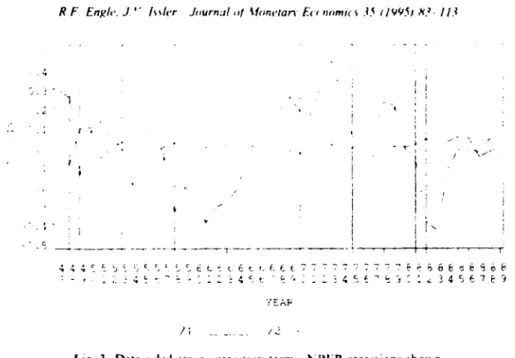
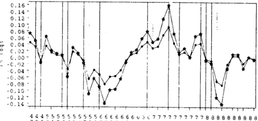
The multivariate procedures described in Secticn 2 were applied to sectoral per-capita real GNP. Per-capita data are used since the theoretical model discussed in the previous section is that of a representative agent Data consist of yearly (lop) sectoral real GNP divided by total population. and IS available from 1947 to 1989.3 Sectors arc a subdivision of private GNP as follows: Agriculture, Forestry & Fisheries A. Construction Con. Mining Min. Wholesale and Retail Trade. W. Manufacturing M. Transportation dnd Public Utihties T. Finance. Insurance & Real Estate I.. and Servkes 3.’ A plot of the data set appears in Fig. I. Most series show the familiar upward trend of macroeconomic variables. it seems however that they are trending at different rates, e.g.. Agricul- ture and Transportation. Fig. 2 shows sectoral GNP growth rates. In an amazing contrast with Fig. I. it seems that growth rates across sectors have

‘All dala wcrc cxtractcd from C’III~XN .md are cnprc\uzd K -vv tam IV82 pricey

‘1 ncrc have been cntlclsms of these particular dara WI as well as a response to them b) the Bureau of Economic Analps (BEA): see Survey of Currznt Business I 1988.1991 I an:! rh- references therein. Almost all of the criticism relates to the Manufacturing and Serv&s figure:. :rnd caused a mcthod- ological change by the BEA in 1977. Using a dummy for the pnsl-1977 p-nod WC found no evidence ofstructural change for these I\LO sectors Nc\errhelfi\. there were SIG illcant changes In the growth ralcs for Conslructlon. Wholc\alc and Retall Trade. and FI!I,A;CL We b&eve these statistical tindings arc not related lo rhc mcthodoi,$cal change of IV77 and may JUSr reflect some unknown form of model misspc~ificalion capured In OUI d- c~~os~~rs test. NotIce that rhic exact same data set was used m Durlauft 19891 and Pesaran et al. (i993l and no unusual behavior of the series is reported there.

a very similar shape and are well synchronized. They mostly drop during NBER recessionsS and increase in periods of prosperity.

Durlauf (1989) tested the order of integration of sectoral per-capita GNP and concluded that these data are well approximated by an It 1) process.” If sectoral outputs contain stochastic trends. the next interesting question is to examine whether or not some of these are common across sectors.

Before applying Johansen’s methodology we must examine what type of deterministiccomponents are present in the VAR. This is a crucial step. since the asymptotic distribution of the test statistic depends on possible restrictions on these components. Thus. we first tested whether the VAR contains a dzterminis- tic linear trend. allowing it to have a constant term. We used the Likelihood Ratio (LR) test obtained from the concentrated likelihood function. The LR statistic for this test is 4X.35. which rejects the null that the VAR (and the EC) does not contain a linear trend at usual significance levels.- The next step was to test if the linear trend is present only inside the EC term (null) against the hypothesis that it is present also outside in the EC model (alternative). This test

Table I

(‘olntcgratlnp rcwl~\ Johan\cn’\ I 1’)Xk) mc~hc~I

12-t ‘76 -l7 ‘1 73 2 174.5” -‘X.X** I .I: nicN 7 rc~intcgratin~ vectnrs 1 .!I mot1 6 wmtegratmg vcctnrb 3 at mc’st 5 cointrgrating vectors 3 at most 4 comtegratmp wctors 3 di most 3 somtegralinp. vectors 3 at mo31 2 comtcprating vectors 3 d! most I comtepratinp vectors 32: most0 cointcgrating vectors

corresponds to testing If*(r) versus H(r) in Johtinsen‘s (1992) notation and H2’(r) versus Hz(r) in Osrerwald-Lcnum’s (1992) notation. The test statistic is 20.32. which rcjccts the restricted model at the i”n significance level. As a consequence, when testing for coimegratton. we consider the data as being

approximately well described by B VAR with an unrestricted constant and a linear time trend. Thcreforc. the critical values of the asymptotic distrii,utions for the trace and i,,, statistics correspond to Table 2 in Osterwald-Lenum.

Table I presents Joh,msen’s trace statistic test for the system containing sectoral ourputs. Given the resulrs. we may conclude that :here are either two or three cointegrating \ectors. To avoid the risk of tinding too much cointegration. typical of large systems. and since the third cointegration vector is only margi- nally significant. we opted for using only two cointegrating vectors in our

“In thts cast. the Vcctw \lA rcprewntatwn of the s!stcm has d ItneAr time trend dnd also a quadratic time trend A\ J comequence. the EC term\ are trend-staticnary. See Johansen tl993.

analysis.’ The estimates of these two cointegration vectors, using the modified VAR representation, are trend-stationary. as expected. In order to extract their deterministic components we run them on a constant and a linear trend. The detrended cointegrating vectors (Z;, = rljq,, i = I, 2) ate plotted in Fig. 3. They both appear to be well-behaved long-run relationships.

Finding a small number of cointegrating vectors rules out the possibility that sectoral o&put data have one common stochastic ::end. Indeed. since the rank of the cointegrating space is 2. the eight sectors will share six idiosyncratic common trends. This finding is consistent with the evidence found in Durlauf (1989). which notes that OIW should not expect to find very different sectors sharing common stochastic trends if these arise from technology shocks. As he notes, a technological improvement in Agriculture does not imply improvement in Manufacturing. due to limited spill-over effects across these sectors.

Table 2 presents the estimates of!he VECM conditioning on two lags of the endogenous variables. This ccrresponds to a VAR of order 3. Tahich. with yearly data. should be enough to capture the dynamics of the system. The VECM estimates are satisfactory. and all residuals passed autocorrelation and normal- ity tests, a desirable feature since Johansen’s test assumes independent Gaussian errors. Table 3 displays system significance levels for each regressor. Inclusion of up to two lags of the endogenous variables seems justified. Notice also the high

c. += 5 s, - .+ =c -c, -- 2s --r. - i i i L -t -=

t Pr > t Rcprcww 17.26 0 0000 LXI 0. I 34x 2 55 00427 5 51 anMY 2 JO 0.054 I 0 x4 0.5813

explanatory powe-l of the time trend in the system. corroborating the evidence of

the LR test previously conducted.

Results of the canonical correlation analysis are presented in Table 4.“’ As

noted belorc. the cofeature rank will be equal to the number of statistically zero

canonical correlations. At the 59/o level. we conclude that the rank of the

cofeature space is 6. This tmplies that eight sectors will share only two idiosyn- cratic serially correlated cycles. Thus. we shouid observe a very similar cyclical

uchavior for different sectors. This result is not surprising. given the similar

pattern of sectoral GNP growth presented in Fig. 2. This feature of the data set exemplifies the basic thrust behind Burns and Mitchell’s (1946) research and is

cited as a styliLed fact in Lucas (1977) and emphasized in Long and Plosser

( 1983. 1987).

Table 5 shows the bases for the cointegrating and cofeature spaces. The basis

for the cointcgrating space is spanned by the two estimated cointegrating

vectors and that for the cofeature space by the six estimated cofeature vectors.

Since these bases form a nonsingular matrix. i.e., N = r + s. we can use these

estimates to construct trends and cycles as discussed above.

Trend and cycle estimates are presented in Figs. 4 through IO and Table

6 presents a summary statistic of the data and these estimates. Since we want to

“‘The F-test used in this table p:widc~ better small sample results than the usual ;/‘ upproximation (see Rao. IY73).

I‘ablc 4

Canonical correlation anaiys. common cycle+ le41 -.. Squared canonical correlations (~tf\ Pr > F 0.9674 0.ooo1 0.8949 0.0113 0.7464 0.419x 0.5855 0.7237 0.5130 0.78$2 0.4367 0.808X 0.3876 0.7922 0.2775 0.7847 ___._ -_- _.__ __---.. ..--. _ ____ --_--._ -.---. __- Null hyporhcw

C’urrcnl and all smaller (,I,) arc zero Current and all smaller (rr,) arc zero Current and all smaller (jr,) arc zero Current and all smatler tp,) arc zcr) Current and all smaller p,) are zero Current and all roller r JJ. ) are zero Current and all smaller (!I,) are zero Current and all smaller ()o,) arc zero

Table 5

Bases for the cofeature and comtcgrating spaces _

Weights

.__ _---- .__,__.. - _... .__ . . .- . . . . . .._ _ Bases 1% A, log Win, log Con, log .V, log 7, log H’, log f, lo&! s

___- --- ----..--_.- -__ -.- __ _____ --..-.. _-...- ..__ ___

Cofeal. I 1.00 - 4.40 - 0.48 2.28 2.93 - 9.03 13.39 - 3.57

Cofeal. 2 0.10 1.00 C.85 - I.86 - 0.63 - 0.49 I.51 3 89

Cofeal. 3 2.40 - 4.09 I.00 9.c7 - 8.55 - 5.00 6.63 14.72

Cokal. 4 - 001 - 0.40 0.47 I.00 - I.51 - I.10 - 3.35 - 0.21

Cnfeal. 5 2.01 - I.14 - 0.13 - 0.79 1.00 I .Ol 4.99 - 1.36

C&at. 6 - 1.03 - 1.1: I.53 - 1.46 0.26 1.00 0.51 234

Coint. I - 0.19 - 0.24 - 0.60 0.58 - I.91 0.86 I.00 075

Coint. 2 0.58 0.h: 0.16 - 0.23 1.75 2.3Y 2.02 IO0

_ _- . _. ..- -_._-._

focus our attention on sectoral cycles, we present only a few sectoral outputs and their respective trends (Figs. 4 through 6). Not surprisingly, since the eight sectors share six idiosyncratic trends. they display a very distinct behavior across sectors. Moreover, many of them seem to be more volatile than sectoral outputs themselves.”

The cyclical components of sectoral output series arc plotted in Figs. 7 through 10. which also include NLER recessions. In these plots. sectors are grouped according to the similarity of their cycles. Five oyt of eight sectoral

“Whenever the covawrnce between trend .tnd qcle IS negattve and big enough m absolute value. mdividual sectoral GNP’s wdl be smoother than then respcctivc trends. This is the case for all sectors but Wholesale~Retail Trade.

Fig. 4. Percaplta constructmn GNP and its trend. NBER recewon\ \hov.n. 8.3 8.2 8.1 8.0 Y 7.3 z7.8 c 7.7 7.5 7.5 7.4 , .3 7.2

cycles conform to NBER recessions and are therefore labe Ld pro-cyclical. They are: Mining. Construction. Manufacturing. Wholesale Retail Trade. and Finance. Three sectors do not conform with NBER rcwessions. with upward movements during those. and are labelled counter-c!,clical. They are: Agricul- ture, Transportation. and Services.

7 4 ‘1 ! .t .? .; 2 7.9 6.3 434555555555566666666667777777777776888888888 ‘39C12~4567Rj01234567890123456789~123456789 YEhi? CUP- -- TREND-- - -

Fig. 6. Per-capita wholevale retail trade GNP and IIS trend. Nl3F.R recessions shown

4445”555555556b6ot 6b66677777777778888888888

-I & ‘( ;, :??55C”~4r,‘3j4567a9~1234 567890!23456789

YEAR

Conslrucl.on- l . .

Fig. 7. Sclecrcd cycles of scctoral per-*xpita GNPs. ;VBER recessions shown.

Examining the cycles of pro-cyclical sectors reveals that these have similar shapes and durations but very different amphtudcs. The sector with the cycle of highest amplitude is Construction. This is not surprising: since Cons!ruction includes housing construction, our evidence is in line with the stylized facts in Lucas (1977). who po ..s out that consumer durable output has relative high

i445555'55555666666EG66-777777i~7~6~890000~

iEVG:234567e3i123456'83~i~3 _{4567e3G123456749}

YEAF

Mlnrng--*** Mdnulaclcricg- t**

Fig. 8. Selected cycles of sectoral per-capita GNPs. NRER recessions shown.

0.16 0.14 0.12 0.10 0.06 0.06 ; c.04 ” c.02 L. 00 L -c.n2 mc.04 -0.36 -0.08 -0.15 -0.12 -0.14 444'555555555i6~6666 7 e j ,‘.? : 2!45c7b9:1;!4567 u~;77777777770a0088800a a3C;234567890:23456769 YEAR

Hkolesdle .Itvtd:l *.'rade- 9.. I‘lrldrlCt: --* l *

Fig. 9. Selected cjclc~ of sectoral per-captta GKPPI, NBER tecesstons shown.

amplitude. Construction is folloxcd by Mining and Manufacturing, with am plitudes roughly half its size. Finally. the lowest amplitudes are found for Wholesale/Retail Trade and Finance, with amplitudes roughly a fifth of that of Construction.

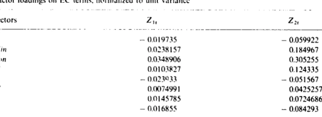
Table 7

Factor loadings on EC terms. normal~zcd to unit variance

Sectors

A -- O.OI 9735 - 0.059922

.\I ill 0.0238157 0. I84967

;-w 0.0348906 0.305255 Al 0.0103827 0. I 24335 T - n.nm33 - 0.05 1567 It 0.0074Y91 0.0425257 F 0.0145785 0.0724686 S - 0.016855 - 0.084293 ..-..- -..-_---. -.. ..-.-.. .-- ._ . . .._ .._. .

All the counter-cyclical sectors have very similar cycles in shape and duration.

They also share a very small cycle amplitude. Moreover. it seems that the shape

of these counter-cyclical cycles is merely an upside down version of the pro-

cyclical ones. These findings reinforce the idea that per-capita sectoral outputs have a common cycle, if not in the statistical sense at least in the economic sense.

Table 7 shows sectoral cycles’ factor loadings of the two EC terms. To make

factor loadings comparable. we normalize the variance of the two EC terms to

unity. For all sectors, the factor loadings of Z2, are much higher than that of Z,,,

suggesting that the variation in sectoral cycles is explained mainly by the

4245555555555666c6666667~7777 78888ti6~~ee

789;i234567~301234~6787c 123456785~123456789

YEAR

Agrlcullcre- l 0. ‘fransporlatlon- l * * Serwces- l A l

Fig. Ii. Sclectcd scctoral per-upita Gh’Ps. ‘4BER ~cL,ss~ons d.own.

cycles it would be surprising to find otherwise. Thus. it seems that although

statistically sectoral cycles are generated by two idiosyncratic components,

economically they are only a result of the variation of Zzr. Thus, we found

a particular rotation of the cointegrating space basis in which only one cointe-

grating vector explains most cyclical pattern of the data set.

To investigate further the findings of counter-cyclical sectors, a plot of the

(log) level series for these sectors is presented in Fig. 1 I. During recessions,

the

behavior of Agriculture is definitely odd: while its series is almost flat, it

increased in four out of seven recessions.

Likewise. Services display little down-

ward sensitivity in recession periods, which is most striking until the 1969-70

recession. Until then per-capita Services output not only increased during

recessions

but even showed no decrease

in its growth rate vis-a-vis neighboring

periods. After 1970. this feature is reversed. Transportation is the only counter-

cyclical series which does not display any unusual behavior for recession

periods. In that sense. observing it to display counter-cyclical behavior is

surprising.

There is some empirical support for our findings of counter-cyclical sectors:

using PSID data. Lougani and Rogerson (1989) found that the influx of workers

into Services increases during recessions and that the outflow of workers from

Services increases during booms. These findings are consistent with countcr-

cyclical behavior for Services, though they do not necessarily imply it. For

Agriculture, Romer (1991). using factor analysis, found evidence that several

agricultm-al goods have short run counter-cyclical behavior (see p. 27). Even

Table 8

Varlancc decomposition of sectoral output innovations. two orthogonallza;ion procedures used

% of the varmnce of sectoral output innovation attributed IO transrlory shocks at horizon (h) Sectors A ,\li,l Con XI T Li’ F s h= I yr 27.4 (0: I 91.9 (10.5) 93.6 (4.9) 99.8 (55.3) 24.9 (19.5) 82.5 (65.8) 91.8 (8.8) 50.5 (7.0) h = 2 yr\. 24.6 II.31 x9.n (I I.‘) X6.3 (1.9) 99.5 (46.9) 18.5 (20X) x9.1 !SY.2) X3.1 (7.1) 41.5 (64 _.-.- _ - h =: 3 yrs. h = 4 yrs. h= x 25.0 (0.5) no 5 (8.9) 12.6 (0.0) 95.9 (40.0) 15.3 (22.5) x7.3 (52.6) 73.1 (4.9) 37. I (4.3) 0 0 0 0 21.0 (1.3) 65.0 (3.7) 55.6 (0.9) 88.6 (32.4) 12.4 (23.0) 71.5 (46.4) 60.0 (I.01 32.3 (3.91 0 0 0 0 --~-.

(a) Obtaminp trend and cycle innovations: one-step-ahead innovations for trends were obtained by first-difTercncing !h::m. For cyc!cs. they arc residuals ofcycle projections on a lagged conditioning =et containing four lag of the EC terms. If-step-ahead trend innovations were obtained by cumulatmg one-step-ahecds. For cycles. they were obtamed by shifting backwards the conditioning MI. (b) Trend and cycle innovations were found to display (signif;iant) negative correlation for all sectors but Wholesalu;Xetail Trade. for which this correlation US statistically zero. Transitory and permanent shocks were obtained by orthogonalizing trend and cycle innovations. These orthogonal shocks were then labelled permanent and transitory shocks to sectoral outputs.

(c) The orthogonalization method used above was: Denote $,’ = (r&,, q!!,)’ as a stack of period I mnovations in sector I and horizon h. whcrc t&, is the innovation in the !rend and $,, is the innovation in the cycle Ttc top number )n Table 7 presents the results of decomposing the variance

off:=(l, l)q$ the total period I innovation in sector i. horizon h. by using a lower trrangular

matrix 0:. such that 0” VAR($,)fI~ is diagonal for all i. in the followirg w;ly: VAR (1:) = VAR[‘I, I) (OF,-’ Dfqf,]. The matrix 0: used was

D” = I 0

- & &, I 1 . a-here VAR(qR) =

The number in parenthcscs performs the same exercise wnh ,I:,’ = ,&,. r&f’ and

Df=

I

h ,k where VAR(rff,) = - fJ,pl OK‘

though her evidence is more compelling for the inter-war era. it holds for the

post-war era as well. Evidence of low Loherence for agricultural output is also

mentioned in Lucas (1977) as a stylized fact of business cycles (see Section 2).

We next investigate the relative importance of transitory and permanent

shocks for the variation ot’ sectoral output data. The results are presented in

Table 8. To construct those numbers, trend and cycle innovations were ortho-

gonalized since they are negatively correlated in most cases. In Table 8, each cell

contains two numbers: the top number represents the relative importance of

transitory shocks when trend shocks come first in the orthogonalizatior, proce-

dure, and the number between parentheses represents the same measure when

cycle innovations are put first. There is of course no consensus on how to

orthogonalize shocks in performing variance decompositions. Nevertheless, in

this specific issue, most authors prefer to put trend innovations first, e.g.. King

et al. (1991), since in theoretical RBC models, productivity (trend) shocks cause

simultaneously trend and cyclical activity.

For given sectors, the results in Table 8 shows that the relative importance of

permanent and transitory shocks may vary depending on the orthogonalitation

procedure. Despite this, some sectors displayed remarkable robustness in rela-

tion to the or!hogonalization procedure employed. For example, the results for

Wholesale/Retail Trade show unequivocally the importance of transitory

shocks, explaming at least 45% of output variation up to the four-year horizon.

Manufacturing is another example where, a? least at short horizons, the bulk of

total variance is explained by transitory shocks. Sectors in which permanent

shocks are unequivocally important are: Agriculture, Transportztion. and Ser-

vices. Notice that these are the counter-cyclical sectors. The remaining sectors.

Construction, Mining, and Finance, have results !hat seem to depend heavily on

the ordering of innovations used, and thus constitute open issues. The picture

that emerges from this analysis is that there is no clear evidence that either

permanent or transitory shocks play a prominent role across all sectors. How-

ever, for essential sectors like Manufacturing and Wholesale/Retail Trade,

transitory innovations are unequivocally important.

Our evidence from the variance decomposition analysis is very different from

that presented in King et al. (1991). In their RBC model, permanent shocks

explained the bulk of the variance of total output innovation. There are two

poisiblc explanations for the difference in results: first, we are using dis-

aggregated data, and second, we are using common-cycle restrictions in per-

forming the trend-cycle decomposition.

As a final investigation, we ‘add up’ sectoral outputs to get some idea of

‘agg:egate’ cycles. Becausc we used data in logs, aggregating :og GNP across

sectors will not give us (log) Private Per-Capita GNP, but in some sense it is still

a measure of agg:egate GNP behavior The sum of sectoral cycles is presented in

Fig. 12. As expected, it conforms to NBER recession periods. Hence, although

some sectors had counter-cyclical behavior, our aggregate

cychcal measure does

l-‘ip 12. <:yclc of privarc pcr-upita G!vP. ‘adding up’, NHER recessions shown.

not show any signs of it. This result is probably caused by the low amplitude of

the cycles for the counter-cyclical sectors.

5. Conclusions and further research

The basic goal of this paper was to re-examine business cycles using a stan-

dard theoretical model and a new econometric technique which allows simul-

taneous discussion of short- and long-run comovement of multivariate data sets.

The results indicate that Sec:ora! Per-Capita GNPs shares a relatively large

number of idiosyncratic common trends hut a reiatively small number of

idiosyncratic common cycles. Thus. irends have a very distinct behavior, where-

as cycles seem almost identical in shape, duration, and timing. Furthermore, at

least in the economic sense, sectoral cycles seem to be generated by a common

component. in this case, the second EC term. The fact that cycles are so similar

for different sectors is remarkable evidence. confirming the basic thrust of Burns

and Mitchell (1946).

The evidence on the importance of permanent versus transitory shocks is

ambiguous. For sectors like Agriculture, Transportation, and Services it seems

that permanent shocks are the most important. However, for Manufacturing

and Wholesale/Retail Trade, it seems that the opposite holds. Under the

theoretical model discussed, sectoral cyclical fluctuations are closely related to

the propagation mechanism at work. On the other hand, trend fluctuations are

closely related to productivity shocks, i.e.. they are a consequence of the impulse

mechanism at work. Although impulses may be very different. causing trends to

differ across sectors, cycles may still be very similar. since the input/output

relationship may work to that end.

Even though the theoretical RBC literature has gone far in modelling together

economic growth and fluctuations under optimizing models, little empirical

evidence has accumulated supporting these models. This paper is a step in this

direction, showing that using production data alone one can describe economic

fluctuations fairly well. Nevertheless, several issues remain open in the business

cycle literature. Of these. the most critical for economic policy is the role of

money: since we showed here that transitory shocks are an important source of

noise for prominent sectors (Manufacturing and Wholesale/Retail Trade), one

possible extens,on of this work is to investigate the relationship between money

and transitory shocks. Although the objectives seem well defined, implementing

this analysis may be difficult due to methodological issues. For this reason, we

decline to pursue it here. Another important issue is the possible link between

long-run shocks and technology. With that regard. our extended model offers an empirical test for Real Business Cycles, since it suggests that the cointegrating

rank of productivity shocks and scctoral outputs should coincide. Although the

objectives are clear once more. how to correctly estimate productivity shocks is

still a controversial matter.

Appendix: Proof of Proposition 1

There is cointegration among the log( Y )‘s if and only if (I - @)(I - A) is

reduced rank. e.g., Engle and Granger (1987). Recall the constant returns to scale

assumption on production functions:

C U,j+hi=l* Vi. and Uij20.

j= 1

If labor is used in all production processes. bi > 0, Vi. thus:

Vi. and Q,, 2 0.

Therefore, A = (Uij) is a nonnegative matrix. Consider now (I -A). Its eigen-

values are 1 - j::, 1 --- 2:. . . . . I - j.1’. where /.‘f. ;:. . . . . j.$ arc the eigenvalues of A. Clearly, if (I - A) is full rank. (I - @)(I -A ) is full rank if and only if (I - @) is full rank. To ),r3-<; L *hc former. it suthces tc show that

Since it implies that all eigenvalues of (I - rl) are nonzero. Eq. (A. 1) follows from

a theorem relating matrix norms and spectral radius. see Lancaster (1969,

t’;,morem 6.13. p. 201). Define

to be the row norm of the matrix A. Then. II A II p 2 max 1 ;.A I.

i

Since 0 I cf;= , 1 Uij 1 < 1. ~/i.ilAil,<l.Thus.max,IiA(<l,and(I-A)isfull

rank. Therefore, (I - A )(I - @) is reduced rank if and only if (I - @) is reduced

rank. Moreover, rank(l - @)(I - A) = rank(l - @). and the result follows.

References

Ahn. S.K. and G.C. Reinsel. 1988. Nested reduced-rank autoregression model for multiple time series. Journal of the American Statistical Association 83, 849. 856.

Anderson, T.W., 1984, An introduction to multivariate statistical analysis (Wiley, New York. NY). Beveridge, S. and C.R. Nelson, 1961. A new approach to decomposition of economic time series into permanent and transitory components with particular attention to measurement of the ‘business cycle’. Journal of Monetary Economics 7. 15 1 .174.

Blanchard, O.J. and D. Quah. 1989. The dynamic effects of aggregate supply and demand dis- turbances. American Economic Review 79. 655 673.

Burns, A.F. and W.C. Mitchell, 1946. Measuring business cycles (National Bureau of Fconomic Research. New York, NY).

Campbell, J.Y. and N.G. Manktw, 1987. Permanent and transitory components in macroeconomic fluctuations, American Economic Review 77. I I 1 117.

Cochrane. J.H., 1988, How big is the random walk in GNP?. Journal of Political Economy 96. 893-920.

Cochrane. J.H.. 1991, Univariate vs. multivariate forecasts of GNP and stock returns: Evidence and implications for the persistence of shocks, detrending methods. and tests of the permanent income hypothesis, Paper presented on the NBER Meeting on Economic Fl.:ztuations. Feb.

Deusenberry. J.S., G. Fromm, L.R. Klein. and E. Kuh, 1965, eds.. The Brookings quarterly econometrics model of the United States (Rand McNally, Chicago, IL).

Durlauf. S.N., 1989. Output persistence, economic structure. and the choice of stabilization policy, Brookings Papers in Economic Activity 2, 69 136.

Durlauf, S.N.. 1993, Time series properties of aggregate output ductuations. Journdl of Econo- metrics 56. 39-56.

Engle, RF. and C.W.J. Granger, 1987, Cointegration and error correction: Representation. estima- tion and testing, Econometrica 55, 251.-276.

Engle, R.F. and S. Kozicki, 1993, Testing for common features, Journal of Business and Economic Statistics 1 I. 369- 395, with discussions.

Evans, G., 1989, Output and unemployment dynamics in the United States, Journal of Applied Econometrics 4. 213 237,

Granger, C.W.J.. 1983, Co-integrated variables and error correcting models. Discussion paper 88-13a (University of California -- San Diego. La Jolla. CA).

Granger, C.W J., 1986. Devclopmcnt\ in the 31udy of cointegrated variables. Oxford Bulletin of Economics and Statistics 48. 2 I3 228.

Issler, J.V. and F. Vahid. 1993. Common cyr ‘es i!l macroeconomic aggregates. Working paper (Graduate School of Economics EPGE, Gctulio Vargas Foundation, 2iq de Janeiro).

Johansen. S.. 1988, Statistical analysis ofcointegrating vectors. Journal of E,.,nomic Dynamicg and Control 12. 231 254.

Johansen, S.. 1992, The role of the constant and hnear terms irl coir :egratitin analysis ornonstation- ary variables, Unpublished manuscript (University of Copenhagen, Copnhagen).

King, R.G.. C.1. Plosser snd S. Rebelo, 1988, Production, growth and business cycles. II. New directions. Journ,! $lf Monetary Economics 21. ?0%341.

King. R.G.. Cl.. P!osser. J.H Stock. and M.W. Watson, 1991, Stochastic trends and economic fluctuations. American Economic Review 81. 819 -840

Kydland, F. and E. Prescott. 1982, Time to build and aggregate fluctuations, Econometrica 50. 134s - I37O.

Lancaster. P., 1969. The theory ol matrices (Academic Press, New York, NY).

Long, J.R. and C.I. Plosser, 1983. Real business cycles, Journal of Political Emnomy 91. 39. 69. Long, J.B. and C.I. Plosser, 1987. Sectoral vs. aggregate shocks in the business cycles. American

Economic Review 77, 333-336.

Lougani. P. and R. Rogerson, 1989. Cyclical fluctuations and sectornl reallocation: Evidence from PSID. Journal of Monetary Economics 23. 259.-273.

Lucas. R.E.. Jr., 1977, Understanding business cycles. Carnegie Rochester Conl:,CIICe Series on Public Policy 5, 7 - 29.

Mankiw. N.G.. 1989. Real business cycles: A new Keynesian perspective. .taurnal of Economic Perspectives 3, 79-90.

Nelson, C.R. and C.I. Plosser. 1982, Trends and random walks in rr lcroeconomic time series. Journal of Monetary Economics 10. 139- 162.

Osterwald-Lenum, M 1992. A note with quantiles of the asymptotic distribution of the maximum likelihood c&tegration rank test statistics, Oxford Bulletin of Economics and StatistiLs 54, JOI- 472.

Pesaran, M.H., R.G. Pierse, alld K.C. Lee, 1993. Persistence, cointegration and aggregation: A disaggregated analysis of output fluctuations in the U.S. economy. Journal of Econometrics 56. 57 -88.

Prescott, EC.. 1986. Theory ahead of business<ycle measurement, Carnepc Rochester Conference Series on Public Policy 25, I I -44.

Rao, C.R., 1973. Linear statistical inference (Wiley. New York. NY).

Romer. CD., 1991. The cyclical behavior of Individual production wries, Quarterly journal of Economics 106. l--31.

Stock, J.H. and M.W. Watson. 1988. Testing for common trends. Journal ofthe American Statistical Association X3. 1097 1107.

Survey of Current Business. July 1988 (Bureau of Econom!c Analysis, Department of Commerce. Washington. DC) 132- 133.

Survey of Current Business. Jan. 1991 iBureau of Economtc Analysis, Department of Commerce. Washington. DC) 23 37.

Tiao, G.C. and R.S. Tsay. 1985. A canonical correlation approach to modelling multivarIate time series. Proceedings of the Business and Economics Statistics Section. American Statlctlcal Associ. ation. I IZ- I20.

Vahid, F. and R.F. Engle. 1993, Common trends and common cycles. Journal of Applied Econo- metrics 8. 341 360.

Watson. M.W., 1986. Univariate dctrending methods with stochastic trends. Journal of Monetary Economics IX. 49. 75.