Analysis of pick-up and delivery and dial-a-ride
problems dynamiza"on methods and benchmark
instances
Renan Artur Lopes Eccel1, Rodrigo Castelan Carlson2
1Federal University of Santa Catarina, [email protected] 2Federal University of Santa Catarina, [email protected]
Recebido:
5 de julho de 2020
Aceito para publicação:
15 de outubro de 2020 Publicado: 16 de novembro de 2020 Editor de área: Renato Lima ABSTRACT
The available benchmarks for the dynamic versions of the Pickup and Delivery Problem with Time Windows (PDPTW) and the Dial-A-Ride Problem (DARP) do not share the same characteris"cs and may not cover all the range of characteris"cs of real situa"ons. We analyze sets of instances of the dynamic PDPTW (DPDPTW) and the dynamic DARP (DDARP) currently available for use, and the methods used to generate them from sta"c instances. We apply each dynamiza"on method to each of the sta"c instances that were originally used by these methods. The resul"ng dynamic instances are analyzed with the measures of degree of dynamism and urgency, as well as with the number of sta"c re-quests and the correla"on between lower limits of the pickup "me window and the requests arrival "mes. The results show that the obtained dynamic instances present low variability in the degree of dynamism and urgency, irrespec"ve of the method or sta"c instance used for dynamiza"on.
RESUMO
As instâncias de benchmark disponíveis para as versões dinâmicas do problema de co-leta e entrega com janelas de tempo (PDPTW - Pickup and Delivery Problem with Time Windows) e do problema dial-a-ride (DARP - Dial-A-Ride Problem) não compar"lham as mesmas caracterís"cas e não necessariamente cobrem todas as caracterís"cas de situ-ações reais. Analisa-se conjuntos de instâncias de PDPTW e DARP dinâmicos (DPDPTW e DDARP) atualmente disponíveis para uso e os métodos usados para gerá-los a par"r de instâncias está"cas. Cada método de dinamização é aplicado a cada instância está"ca originalmente usada por eles. As instâncias dinâmicas resultantes são analisadas com as medidas de grau de dinamismo e urgência, bem como pelo número de pedidos está"cos e a correlação entre os limites inferiores das janelas de tempo de coleta e os instantes de chegada dos pedidos. Os resultados mostram que os conjuntos estudados apresen-tam baixa variabilidade de grau de dinamismo e urgência independentemente do mé-todo ou da instância está"ca usados para a dinamização.
Keywords: Dynamiza"on. Benchmark instances. DDARP. DPDPTW. Palavras-chaves: Dinamização. Instâncias de benchmark. DDARP. DPDPTW. DOI:10.14295/transportes.v28i4.2412
1. INTRODUCTION
Dynamic vehicle routing problems have been the subject of research for nearly three decades (Psaraftis et al., 2015). Derived from classic vehicle routing problems (VRP), such as the dial-a-ride problem (DARP) and the pickup and delivery problem with time windows (PDPTW), the dynamic problems seek to model cases in which one or more parameters of the problem are not fully known a priori and may vary during the period of operation.
Among the dynamic vehicular routing problems, the dynamic dial-a-ride problem (DDARP) (Psaraftis, 1988) and the dynamic pickup and delivery problem with time windows (DPDPTW) (Dumas et al., 1991) are of great interest for the development of new urban transport technol-ogies. These are the problems that need to be solved when a dynamic ride-sharing service is
needed (Agatz et al., 2012; Alonso-González et al., 2018), or when timely parcel delivery is re-quired (Pankratz, 2005). Currently, some companies provide such services (UberPool, Via, UBus, UberEats, Rappi, etc.). However, with the expected technological advances in the area of connected vehicles, automated driving and the diversi6ication of public transport introduced mainly by mobility as a service (MaaS) systems, algorithms for solving DDARPs and DPDPTWs in less time and providing a better result are increasingly necessary (Fulton et al., 2017).
The idea of using computational experiments in this context is to be able to generate results on the ef6iciency and computational time required by different algorithms and methods that are available for the solution of these problems in order to compare their performance. In order to obtain results that can be compared between articles without the need of rerunning the com-putational experiments already performed by other authors, it is necessary that the same sce-narios are used. Moreover, a series of characteristics should be present in these scesce-narios to re6lect real applications (Uchoa et al., 2017). In the area of static VRP it is common to have ex-tensively used sets of canonical scenarios that facilitate the comparison between algorithms (Mendoza et al., 2014, Uchoa et al., 2017). These are called sets of benchmark instances. How-ever, the benchmark instances for dynamic vehicle routing problems (Pillac et al., 2013; Maciejewski et al., 2017) do not share the same characteristics and may not cover the full range of characteristics from real situations.
The purpose of this article is evaluating benchmark instances of DDARPs and DPDPTWs that are accessible and available for use and the dynamization methods used for obtaining these dynamic instances from static instances. The focus is on how requests are distributed through-out the systems’ period of operation. Thus, two measures proposed by Van Lon et al. (2016), urgency and degree of dynamism, that help in identifying the temporal characteristics of the instances, are used. The dynamization methods are brie6ly described. Then, each method is ap-plied to different sets of static instances and the degree of dynamism and urgency of the result-ing dynamic instances are evaluated. Given that a good set of dynamic instances must cover most of the degree of dynamism and urgency spectrum, our aim is to evaluate the dispersion of these metrics for some datasets. The number of static requests and the correlation between lower limits of the pickup time window and the requests arrival times are also analyzed. It is shown that dynamic instances analyzed present low variability in their measures of degree of dynamism and urgency.
It is expected that the provided results will ease the process of searching and selecting sets of dynamic instances for use in computational experiments and in testing new algorithms. Al-ternatively, the results may assist in the selection of a method for generating dynamic instances that are more appropriate to the research goal.
The de6initions of the problems of interest are presented in Section 2. In Section 3, the sets of dynamic benchmark instances and dynamization methods are described. Section 4 intro-duces the measures of degree of dynamism and urgency, followed by an assessment of the dy-namization methods and the dynamic instances obtained from static instances. Finally, Section 5 provides the concluding remarks.
2. FORMAL DEFINITION OF DYNAMIC PROBLEMS
This section presents the formal de6initions of the DARP, the PDPTW, the DDARP and the DPDPTW based on Cordeau and Laporte (2003). To this end, 6irst the de6inition of the static DARP is presented, based on which the other three problems are then de6ined.
2.1. DARP
The DARP consists of a set of passenger requests for transport between different pickup and delivery locations that must be met by a 6leet of vehicles capable of carrying more than one passenger at a time. The goal is to 6ind a set of routes for the vehicles in the 6leet that minimizes the time and/or cost to ful6ill all requests.
Each request has a pickup location and an associated time window that identi6ies the upper- and lower-time limits in which the user wishes to be picked up for the trip. Similarly, the transport request also has a passenger destination and a time window for delivery. Despite of having de6ined a time window for the desired start and end of his trip, the passenger also ex-pects his journey to take no more time than what he considers acceptable.
The DARP can be de6ined by a complete directed graph ( , ), where are the nodes and
are the arcs of the graph, with = ∪ ∪ , , = , … , , = , … , ,
and the number of requests. The subsets and contain, respectively, the pickup and deliv-ery nodes of the requests, while the nodes and represent the origin and destination of the vehicles. All vehicles in the 6leet must start their routes at node and end them at node
. To each request ∈ 1, … , a pickup node ∈ and a delivery node ∈ are
associated. To each arc , ∈ is associated a cost ( , ) and a travel time ( , ).
Each vehicle ∈ , with the set of available vehicles, has a capacity ! and a maximum total route time "!. To each node ∈ there is an associated load # and a non-negative service
time $ , with $ = $ = 0 and # = −# .
The pickup time window is de6ined by '( , ) *, with ( and ) denoting the lower and upper limit for the start of pickup at node , respectively. Analogously, the delivery time window is given by '( , ) * for delivery at node . The maximum travel time of a request, , , is determined by the amount of time the passenger considers acceptable for his journey.
Finally, a time interval, called planning horizon, is de6ined as '0, -*. The time that corre-sponds to instant zero represents the beginning of the operation, when all vehicles are in the initial node ( ) and all users are waiting to be picked up at their respective origins. The time instant - denotes the end of the operation, when all the vehicles have completed their routes and are at the 6inal node ( ), having taken all users from their respective origins to their destinations. The time windows of every node must be contained in the time interval '0, -*.
2.2. PDPTW
As in the DARP, the PDPTW has a set of transport requests with different origins and destina-tions and associated time windows. It also has a 6leet of vehicles with the capacity to handle more than one request at a time. However, the requests in a PDPTW refer to the transport of goods instead of passengers. For that reason, the only difference between the de6inition of the DARP and the PDPTW arises (Parragh et al., 2008). In the de6inition of the DARP presented in Subsection 2.1, the parameter , represents the maximum travel time of a request, which limits the total time that a passenger wishes to remain in the vehicle. However, for the PDPTW this restriction is not necessary since the cargo does not suffer any discomfort with the delay in travel time. Therefore, the same de6inition presented previously for the DARP can also be used for PDPTW, however, for the latter, the parameter , = ∞, ∀ ∈ .
2.3. DDARP and DPDPTW
In the de6initions of the DARP and the PDPTW, presented in Subsections 2.1 and 2.2, respec-tively, requests are fully known before solving the problem and stay immutable through the so-lution application. Therefore, they are static problems (Psaraftis, 1988). Differently, dynamic problems receive data in real time during operation. In this case, requests are sent by users at any time between the start and end of the planning horizon, requiring new computation of so-lutions.
In dynamic problems each request has an arrival time 0 , ∀ ∈ , which represents the exact moment the transportation system receives the request’s data. This new data can then be used to recalculate vehicle routes. Because of this, all request arrival times must be less or equal than the lower limit of the pickup time window (( ).
The DARP and the PDPTW de6initions previously described are therefore modi6ied with the addition of this set of parameters, i.e., the requests arrival times, and the corresponding con-straint. This results in a succinct de6inition of their respective dynamic problems: the DDARP and the DPDPTW.
3. SETS OF BENCHMARK INSTANCES AND DYNAMIZATION METHODS
This section presents the sets of dynamic benchmark instances of the DDARP and the DPDPTW and the dynamization methods used to derive them from static benchmark instances. Berbeglia
et al. (2012), Pureza e Laporte (2008), Pankratz (2005) and Fabri and Recht (2006) apply each
a different method to convert static instances into dynamic ones. These sets were chosen be-cause the related data is freely available for access on the internet (Pankratz e Krupczyk, 2009). The static characteristics of the instances are not presented in this article; for detailed infor-mation, the reader is referred to the corresponding articles cited in each of the following sub-sections. Tables summarizing the static instances are provided by Eccel (2019).
Two other sets of dynamic instances are freely available. One set was created arti6icially in order to replicate the behavior of an urban environment, with peak hours and a concentrated demand in the city center (Gendreau et al., 2006). The other set is based on real data, collected from one medium and one large sized courier companies operating in Vancouver, Canada (Mi-trovic-Minic and Laporte, 2004). Since these two sets do not involve dynamization, they are not analyzed in this paper. The reader is referred to Eccel and Carlson (2019) for an analysis of urgency and degree of dynamism of these two sets.
3.1. DDARP instance sets and method proposed by Berbeglia et al. (2012)
Berbeglia et al. (2012) used two different sets of instances for their computational experiments, each derived from different sets of static instances. In the 6irst set they used the static instances proposed by Ropke et al. (2007) as a basis. In the second, the static instances presented by Cordeau and Laporte (2003) were used. In both cases, they chose to use instances whose num-ber of requests was forty or more.
Both sets were dynamized using the following technique. A pair of parameters (1, 2) was de6ined. Parameter 1 ∈ '0,1* de6ines the percentage of requests known at the beginning of the time horizon. If 1 = 0 the problem is completely dynamic. If 1 = 1 the problem is completely static and all requests are known in advance. The parameter 2 represents a time interval
for the system to react to dynamic requests. That is, the interval between the arrival of a request and its pickup is always greater than 2.
Given a request , the value 0345675 is an arrival time upper limit which enforces the possibility to serve the request in time. Thus:
0345675= min;) , ) −
( , )− $ <. (1)
Therefore, the request arrival time can be de6ined as:
0 = 0345675− 2 (2)
Berbeglia et al. (2012) use the parameters 1 = 0.25 and 2 = 60 min for the dynamization of the set of instances presented by Ropke et al. (2007). For the set of instances from Cordeau and Laporte (2003), the conversion into a set of dynamic instances used the parameters 1 = 0.25 and 2 = A(60; 240), with A(0; D) representing a random variable with uniform distribution in the interval '0, D*. In addition, Berbeglia et al. (2012) uses the Euclidean distance as a value for the travel time between two points, thus ( , ) can be computed using the distance between
and .
In this paper, when the dynamization method by Berbeglia et al. (2012) is applied, we make 1 = 0, since our interest is to obtain completely dynamic cases. Note, however that choosing 1 = 0 does not mean that static request will not exist, but just that this type of request is not enforced. The same values of 2 are used.
3.2. DPDPTW instance sets and method proposed by Pureza and Laporte (2008)
The DPDPTW instances proposed by Pureza and Laporte (2008) were generated by dynamizing the static instances with 100, 200 and 400 nodes (50, 100 and 200 requests) proposed by Li and Lim (2003). Pureza and Laporte (2008) de6ine the request arrival time as:
0 = min;( , max;A(1; 5), ) − ( , )− 2<<, (3)
with ( , ) the average travel time of a vehicle that wants to pick up the request . For each of the PDPTW instances, four DPDPTW instances were generated with different reaction time values (2) equal to 0, 100, 200 and 300.
3.3. DPDPTW instance sets and method proposed by Pankratz (2005)
Pankratz (2005) created two sets with a total of 5600 DPDPTW instances. These instances are based on the 100-node PDPTW instances proposed by Li and Lim (2003). Pankratz (2005) dy-namized the instances by calculating the last arrival time for each request ∈ by:
0345675∶= min;) , ) −
( , )− $ < − ( , ). (4)
Subsequently, each request is assigned an arrival time calculated by:
0 = H ∙ 0345675, (5)
with H ∈ '0.1,1.0*, in steps of 0.1. Like 2, the parameter H also represents a reaction time to dynamic requests, however, instead of being a value of time it is a percentage. For each of the 6ifty-six PDPTW instances, ten DPDPTW instances were generated, one for each of the possible values of H, resulting in a total of 560 dynamic instances.
3.4. DPDPTW instance sets and method proposed by Fabri and Recht (2006)
The instances proposed by Fabri and Recht (2006) were based on all PDPTW instances of Li and Lim (2003). To make the instances dynamic, they draw the request arrival time from:
Compared to the previous three dynamization methods, this method does not show an ex-plicit parameter for the reaction time to dynamic requests. This is imex-plicitly modelled using the uniform distribution for the de6inition of the request arrival time.
4. ANALYSES OF BENCHMARK INSTANCES AND DYNAMIZATION METHODS
In this section, we introduce the metrics of urgency and degree of dynamism proposed by Van Lon et al. (2016). These metrics are then used for analyzing the dynamization methods de-scribed in Section 3. We applied the four dynamization methods by Berbeglia et al. (2012), Fabri and Recht (2006), Pankratz (2005), and Pureza and Laporte (2008) to all the static instances in Ropke et al. (2007), Cordeau and Laporte (2003), Li and Lim (2003). This resulted in twelve generated dynamic datasets (sets of dynamic instances) to be evaluated with respect to urgency and degree of dynamism. Because some methods, nevertheless, create static requests, their number is computed. As seen in the previous section, the lower limit of the pickup time widow plays an important role in some methods, therefore their correlation with the requests’ arrival times is also analyzed.
4.1. Degree of dynamism
For Van Lon et al. (2016), the degree of dynamism measures the continuity with which transport requests are received by the system. In other words, it relates to the distribution of request arrival times within the planning horizon. Therefore, the more distributed the request arrival times are, the higher the value of the degree of dynamism is. The degree of dynamism ranges from zero to one, with zero being a scenario in which all requests take place at the same time and one a scenario in which requests are equally spaced within the planning horizon.
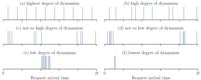
Figure 1 shows six different hypothetical instances, each one with a different degree of dy-namism. In the 6igure, each graph depicts a scenario with a total of ten dynamic requests. In Figure 1(a), all arrival times are equally spaced and evenly allocated at the planning horizon. This scenario is considered to have a high degree of dynamism (equal or close to 1). From Figure 1(b) to Figure 1(f) the intervals between arrival times of request are gradually decreased cre-ating clusters of requests that, eventually, become a single cluster. In Figure 1(f) all the request arrival times are roughly equal, thus the corresponding scenario has low degree of dynamism (equal or close to zero) (Van Lon et al., 2016).
In order to calculate the dynamism of an instance Van Lon et al. (2016) de6ine a list (∆) of interarrival times:
∆= K , K , KL, … , K M , = ;0 − 0 | O = + 1 ∀ ∈ <, (7)
with K the interarrival time between the requests and + 1 and |∆| = − 1 the list size. Note that the interarrival times in ∆ correspond to intervals for which the transportation system is unchanged in terms of solution. Furthermore, the list is organized in chronological order.
Van Lon et al. (2016) also de6ine a perfect interarrival time, Q, that represents the scenario of 100 percent degree of dynamism:
Q = R. (8)
This enables the computation of interarrival times deviation, S , with respect to the perfect interarrival time: S = T Q − K , if = 1 and K < Q Q − K + XMYZ X ∙ SM , if > 1 and K < Q 0, otherwise. (9) Then, the total scenario deviation is de6ined as:
c = d S
|e| f
.
However, the total scenario deviation should be normalized by its maximum possible value (c̅), which is de6ined by:
c = d Sh |e| f . with: Sh = Q − i XM YX Z∙ SM , if > 1 and K < Q 0, otherwise. (12)
Van Lon et al. (2016) de6ine the degree of dynamism as:
j = 1 −kk (13)
where the division of c by c̅ represents the normalized total scenario deviation of interarrivals despite the perfect case. The value of this division is contained in the interval '0, 1* and has high values for low degrees of dynamism. To render the measure more intuitive, Van Lon et al. (2016) subtracted this value from 1.
4.2. Urgency
The urgency (l ) represents the reaction time available to the transport system so that it can ful6ill the request and is given by (Van Lon et al., 2016):
l = ) − 0 . (14)
Figure 2 shows two requests with distinct values of urgency. The case in Figure 2(a) repre-sents a scenario with high urgency whereas the case in Figure 2(b) reprerepre-sents a scenario with low urgency. Note the longer l for the latter.
Since the urgency value represents the available reaction time of one request, low values of l are related to high urgency requests. The mean and standard deviation of the urgency of all requests gives a measure of urgency for a given instance.
(10)
Figure 2. Hypothetical requests with distinct values of urgency (Van Lon et al., 2016)
4.3. DistribuAon of the degree of dynamism and urgency
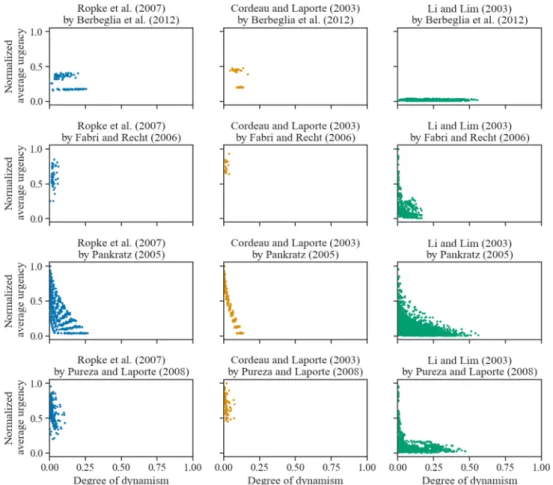
Each graph in Figure 3 represents the result of a different generated dynamic dataset. Each point in the graph corresponds to the normalized average urgency (vertical axis) and dynamism (horizontal axis) values of one dynamic instance of a set. The average urgency normalization was done in such a way that the value zero represents an average urgency equal to zero and the value one represents the highest average urgency found within all the generated dynamic datasets.
Figure 3. Scatter plots of normalized average urgency and dynamism for all instances of each generated dynamic dataset
The accumulation of points in Figure 3 shows the lack of diversity in the generated dynamic datasets. None of the generated dynamic datasets evenly cover the dynamism and urgency spec-trum. Most of them have low degree of dynamism, while the slightly larger degrees of dynamism obtained from the static datasets of Li and Lim (2003) may be related to the characteristics of the instances.
Clearly, Pankratz (2005) obtained a better distribution of values in the whole range of ur-gency. The values of urgency seem to be more related to the method used, although again the static dataset from Li and Lim (2003) seems to result in dynamic instances covering almost the whole range of urgency values, except when the method by Berbeglia et al. (2012) is used. As matter of fact, in all three dynamic datasets created using the method by Berbeglia et al. (2012) the urgency values accumulated in one or two clusters. This is a re6lex of using only a small set of values for β. In the case of the static datasets by Ropke et al. (2007) and Cordeau and Laporte (2003) it is easy to distinguish between the instances that are generated using a 6ixed value of
β (the lower cluster) and the ones that are generated using a uniform distribution (the upper
cluster).
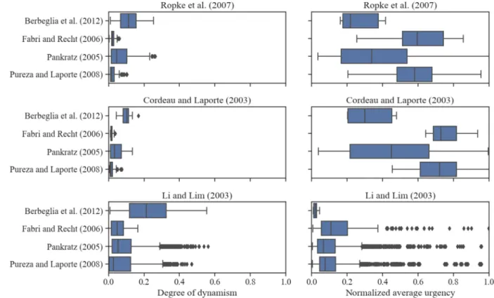
Figure 4 shows the same values of degree of dynamism (left) and urgency (right) shown in Figure 3, however in the form of a box plot. The left side of each box represents the 6irst quartile , i.e., to its left lie the 25% instances with lowest degree of dynamism (or urgency). The right side of the box represents the third quartile L, i.e., to its left lie the 75% instances with lowest degree of dynamism (or urgency). Therefore, the boxes cover, for each case, the degree of dyna-mism (or urgency) of 50% of the instances. The median of the degree of dynadyna-mism (or urgency) of each dynamic dataset is marked by a vertical line within the box and the lower (,,) and upper (m,) limits are delimited by the vertical line segments outside the boxes, whose values can be calculated by:
,, = − 1.5 ⋅ o p, (15)
m, = L+ 1.5 ⋅ o p, (16)
with the interquartile range given by:
o p = L− . (17)
The diamonds indicate outliers, i.e., values not contained in the interval ',,, m,*.
All generated dynamic datasets have medians of the degree of dynamism of at around 0.2 or less and a high concentration of instances with degree of dynamism of less than 0.3. It is worth noting that the greater the dynamism, higher is the number of optimization calls. Therefore, dynamic datasets with a concentration of low degree of dynamism can bene6it algorithms that return good results at the cost of a long computation time.
Another point to be highlighted is the scarcity of instances with dynamism between 0.45 and 0.6. Van Lon et al. (2016) claim that this range of dynamism values occurs in scenarios gener-ated by homogeneous Poisson distributions. Bearing in mind that the arrival of travel requests in real world DARP systems happens in a way that resembles a homogeneous Poisson distribu-tion (Schilde et al., 2011), the lack of instances with these dynamism values hinders the analysis of realistic scenarios.
The normalized average urgency boxplot in Figure 4 shows a diversity of distributions. Li and Lim (2003), despite having a good coverage of urgency spectrum, show an accumulation of low urgency values, which over evaluate algorithms that value short-term results.
4.4. CorrelaAon between lower limits of pickup Ame windows and requests arrival Ames
By the description of dynamism brie6ly presented in Section 4.1, one can note that the interar-rival times between requests are the main factors determining the degree of dynamism of an instance. Therefore, a dynamic dataset will have instances whose degrees of dynamism are dif-ferent from each other, if the arrival times distribution is difdif-ferent between instances (Van Lon
et al., 2016).
However, in Section 3, most of the dynamization methods do not allow the diversi6ication of time intervals between instances. The only exception being Pankratz (2005) (Section 3.3), who varies the value of 2 ensuring that one static instance will generate a couple of dynamic in-stances with different reaction times. Nevertheless, Pankratz (2005) still failed to achieve a very wide range of dynamism (Figures 3 and 4).
Among the dynamization methods presented in Section 3, it is common to use pickup time window limits to obtain arrival times, which makes the time windows distribution affect di-rectly the arrival times distribution. Therefore, if the distribution of time window limits has an accumulation of values, there is a possibility that this accumulation will be passed on to the arrival times distribution.
Figures 5 and 6 show the histogram and cumulative frequency of lower and upper limits of pickup time windows for the sets of static instances used in this work, all normalized by their respective planning horizon.
Figure 5. Histogram of the lower limits of the pickup time windows for each set of static instances. Values normalized
Figure 6. Histogram of the upper limits of the pickup time windows for each set of static instances. Values normalized
by the planning horizon.
All the histograms in Figure 5 show an aggregation at the beginning of the planning horizon. The accumulated frequency shows that all static instances have more than 75% of their lower limit of pickup time windows before the middle of the planning horizon.
In Figure 6 it is shown that 50% of the requests by Ropke et al. (2007) and Cordeau and Laporte (2003) have their upper limit delivery time windows at the end of the planning horizon, and also have a range (between 0.4 and 0.9) where there is no occurrence. Since some dynami-zation methods use the upper limit of delivery time window to establish the request arrival time, this “dead zone” can dif6icult the creation of requests with arrival time around this zone.
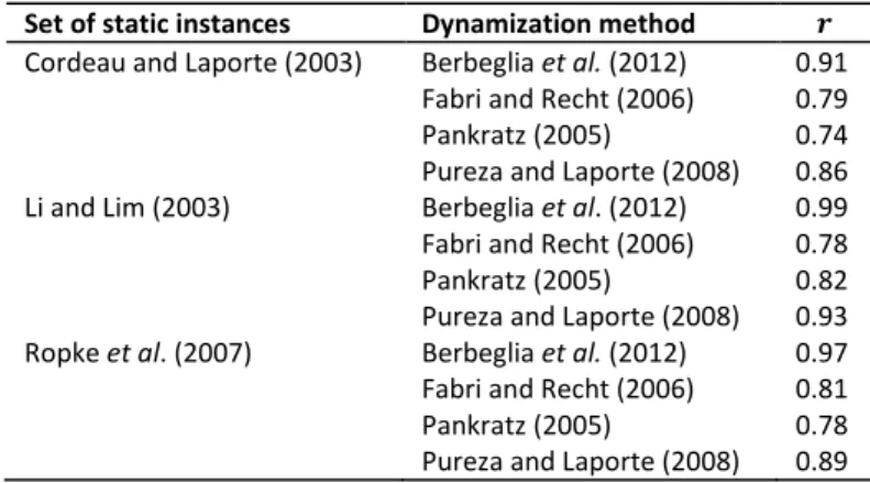
Table 1 shows correlation values between arrival times and pickup time windows lower lim-its. The highest correlations are perceived for the dynamization methods proposed by Berbeglia
et al. (2012) and Pureza and Laporte (2008). The two other methods have a slightly lower
cor-relation, which can be explained by the use of random variables taken from an uniform distri-bution in the dynamization method by Fabri and Recht (2006) and by the reaction time param-eter variation applied by Pankratz (2005).
Table 1 – Correlation values between the normalized arrival times and the normalized lower limits of the pickup time
windows
Set of static instances Dynamization method q
Cordeau and Laporte (2003) Berbeglia et al. (2012) Fabri and Recht (2006) Pankratz (2005)
Pureza and Laporte (2008) 0.91 0.79 0.74 0.86 Li and Lim (2003) Berbeglia et al. (2012)
Fabri and Recht (2006) Pankratz (2005)
Pureza and Laporte (2008) 0.99 0.78 0.82 0.93 Ropke et al. (2007) Berbeglia et al. (2012)
Fabri and Recht (2006) Pankratz (2005)
Pureza and Laporte (2008) 0.97 0.81 0.78 0.89
4.5. Presence of staAc requests
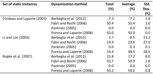
The analysis of arrival times shows that the Fabri and Recht (2006) and the Pureza and Laporte (2008) dynamization methods generate many requests with arrival time equal to zero, which, by de6inition, are considered static requests. Table 2 shows the percentage of requests with ar-rival time equal to zero for all the generated dynamic instances.
Table 2 – Percentage of requests with arrival time equal to zero
Set of static instances Dynamization method Total (%) Average (%) Std. Dev. (%)
Cordeau and Laporte (2003) Berbeglia et al. (2012) Fabri and Recht (2006) Pankratz (2005)
Pureza and Laporte (2008)
7.3 50.4 0.0 50.0 7.2 50.4 0.0 50.0 1.8 1.0 0.0 0.0 Li and Lim (2003) Berbeglia et al. (2012)
Fabri and Recht (2006) Pankratz (2005)
Pureza and Laporte (2008)
3.7 19.9 0.0 19.4 8.5 23.6 0.3 48.5 11.2 27.6 0.1 20.5 Ropke et al. (2007) Berbeglia et al. (2012)
Fabri and Recht (2006) Pankratz (2005)
Pureza and Laporte (2008)
15.8 50.7 0.0 50.2 17.2 50.9 0.0 50.2 8.0 1.8 0.0 0.8
The percentage of static requests is an important feature of instances. They represent an in-itial condition of the system. Therefore, it is a good practice to have a ranging value of static requests percentages in benchmark datasets for testing different initial conditions.
Table 2 shows that most of the generated dynamic datasets fail to cover a good range of static instances percentage. The only two exception being Li and Lim (2003) by Fabri and Recht (2006) and by Pureza and Laporte (2008). The method proposed by Pankratz (2005) does not generate any static instance. However, in his work some additional parameters are used to ad-dress this condition, if needed. It is believed that this side effect is also caused because of the use of pickup and delivery time windows limits combined with the use of static instances that have an accumulated distribution of these values, especially at the beginning of the planning horizon. Therefore, when using dynamization methods, care must be taken that they do not generate too many static requests, which can hinder the analysis of algorithms made to deal with dynamic requests.
5. CONCLUDING REMARKS
This article succinctly presented sets of benchmark instances for the DDARP and DPDPTW and the methods used for generating them from static instances. We performed the analysis using degree of dynamism and urgency metrics proposed by Van Lon et al. (2016) for a series of com-binations of static benchmark datasets and dynamization methods presented. The number of static requests and the correlation between lower limits of the pickup time window and the requests arrival times were also analyzed. It was observed that all the dynamization methods generate dynamic benchmarks with little variability in relation to the degree of dynamism and urgency values for the used static sets. This is mainly caused by the fact that the dynamization methods work with a low variability of parameters and too much dependency on the pickup time window limits. This is an unwanted feature for dynamization methods.
Benchmark instances and dynamization methods with a wide variety of characteristics help to test different aspects of algorithms and can favor the development of more 6lexible methods, which can be used in real situations with less risk of failure (Uchoa et al., 2017).
It is hoped that this paper serves as a basis for other researchers in the 6ield of dynamic ve-hicle routing who are interested in studying the behavior of solution algorithms for DDARP and DDPDTW through computational experiments. It should be noted that all the data from the sets
of benchmark instances that are characterized and analyzed in this paper are freely available for consultation and use, as well as all the source code used for their analysis (Eccel, 2020).
For future work, we suggest an analysis of the spatial factors of the instances, especially the distribution of the pickup and delivery locations. The investigation of new methods for convert-ing static instances into dynamic instances is recommended if more variability of the degree of dynamism and urgency is required.
ACKNOWLEDGEMENTS
The authors acknowledge the support from CAPES and CNPq.
REFERENCES
Agatz, N.; A. Erera; M. Savelsbergh and X. Wang (2012) Optimization for Dynamic Ride-Sharing: A Review. European Journal of Operational Research, v. 223, n. 2, p. 295–303. DOI: 10.1016/j.ejor.2012.05.028
Alonso-González, M. J.; T. Liu; O. Cats; N. Van Oort and S. Hoogendoorn (2018) The Potential of Demand-Responsive Transport as a Complement to Public Transport: An Assessment Framework and an Empirical Evaluation. Transportation Research Record, v. 2672, n. 8, p. 879–889. DOI: 10.1177/0361198118790842
Berbeglia, G.; J.-F. Cordeau and G. Laporte (2012) A Hybrid Tabu Search and Constraint Programming Algorithm for the Dynamic Dial-a-Ride Problem. INFORMS Journal on Computing, v. 24, n. 3, p. 343–355. DOI: 10.1287/ijoc.1110.0454
Cordeau, J.-F. and G. Laporte (2003) A Tabu Search Heuristic for the Static Multi-Vehicle Dial-a-Ride Problem. Transportation Research Part B: Methodological, v. 37, n. 6, p. 579–594. DOI: 10.1016/S0191-2615(02)00045-0
Dumas, Y.; J. Desrosiers and F. Soumis (1991) The Pickup and Delivery Problem with Time Windows. European Journal of Ope-rational Research, v. 54, n. 1, p. 7–22. DOI: 10.1016/0377-2217(91)90319-Q
Eccel, R. A. L. (2019) Problemas Dinâmicos de Coleta e Entrega com Janelas de Tempo: Análise de Instâncias de Benchmark. Dis-sertação (mestrado). Programa de Pós-graduação em Engenharia de Automação e Sistemas, Universidade Federal de Santa Catarina. Florianópolis. Available at: <http://tede.ufsc.br/teses/PEAS0339-D.pdf> (accessed on 19/10/2020).
Eccel, R. A. L. (2020) renan-eccel/instances-DDARP-DPDPTW: v1.2. Available at: <https://zenodo.org/record/4107192> (ac-cessed on 19/10/2020). DOI: 10.5281/zenodo.4107192
Eccel, R. A. L. and R. C. Carlson (2019) Problemas Dinâmicos de Coleta e Entrega com Janelas de Tempo: Análise das Instâncias de Benchmark. 33º Congresso da Associação Nacional de Pesquisa e Ensino em Transportes, ANPET, Balneário Camboriú. Available at: < http://www.anpet.org.br/anais/documentos/2019/Log%C3%ADstica/Log%C3%ADstica%20Ur-
bana%20e%20Planejamento%20e%20Opera%C3%A7%C3%A3o%20de%20Sistemas%20Log%C3%AD-sticos/6_603_AC.pdf> (accessed on 19/10/2020).
Fabri, A. and P. Recht (2006) On Dynamic Pickup and Delivery Vehicle Routing with Several Time Windows and Waiting Times. Transportation Research Part B: Methodological, v. 40, n. 4, p. 335–350. DOI: 10.1016/j.trb.2005.04.002
Fulton, L.; J. Mason and D. Meroux (2017) Three Revolutions in Urban Transportation. Institute for Transportation & Develop-ment Policy, Davis, CA.
Gendreau, M.; F. Guertin; J.-Y. Potvin and R. Séguin (2006) Neighborhood Search Heuristics for a Dynamic Vehicle Dispatching Problem with Pick-Ups and Deliveries. Transportation Research Part C: Emerging Technologies, v. 14, n. 3, p. 157–174. DOI: 10.1016/j.trc.2006.03.002
Li, H. and A. Lim (2003) A Metaheuristic for the Pickup and Delivery Problem with Time Windows. International Journal on Arti5icial Intelligence Tools, v. 12, n. 2, p. 173–186. DOI: 10.1142/S0218213003001186
Maciejewski, M.; J. Bischoff; S. Hörl and K. Nagel (2017) Towards a Testbed for Dynamic Vehicle Routing Algorithms. In: Bajo, J.; Z. Vale; K. Hallenborg; A. P. Rocha; P. Mathieu; P. Pawlewski; E. Del Val; P. Novais; F. Lopes; N. D. Duque Méndez; V. Julián and J. Holmgren (eds.) Highlights of Practical Applications of Cyber-Physical Multi-Agent Systems. Communications in Computer and Information Science. Springer International Publishing, p. 69–79. DOI: 10.1007/978-3-319-60285-1_6
Mendoza, J. E.; C. Guéret; M. Hoskins; H. Lobit; V. Pillac; T. Vidal and D. Vigo (2014) VRP-REP: The Vehicle Routing Problem Repository. Third meeting of the EURO Working Group on Vehicle Routing and Logistics Optimization (VeRoLog). Oslo, Nor-way.
Mitrovic-Minic, S. and G. Laporte (2004) Waiting Strategies for the Dynamic Pickup and Delivery Problem with Time Windows. Transportation Research Part B: Methodological, v. 38, n. 7, p. 635–655. DOI: 10.1016/j.trb.2003.09.002
Pankratz, G. (2005) Dynamic Vehicle Routing by Means of a Genetic Algorithm. International Journal of Physical Distribution & Logistics Management, v. 35, n. 5, p. 362–383. DOI: 10.1108/09600030510607346
Pankratz, G. and V. Krypczyk (2009) Benchmark Data Sets for Dynamic Vehicle Routing Problems. Available at:<https://web.ar-chive.org/web/20120622022350/http://www.fernuni-hagen.de:80/WINF/inhalte/benchmark_data.htm> (accessed on 01/07/2020).
Parragh, S. N.; K. F. Doerner and R. F. Hartl (2008) A Survey on Pickup and Delivery Problems: Part II: Transportation Between Pickup and Delivery Locations. Journal für Betriebswirtschaft, v. 58, n. 2, p. 81–117.
Pillac, V.; M. Gendreau; C. Guéret and A. L. Medaglia (2013) A Review of Dynamic Vehicle Routing Problems. European Journal of Operational Research, v. 225, n. 1, p. 1–11. DOI: 10.1016/j.ejor.2012.08.015
Psaraftis, H. N. (1988) Dynamic Vehicle Routing Problems. In: Vehicle Routing: Methods and Studies. North-Holland, p. 223– 248.
Psaraftis, H. N.; M. Wen and C. A. Kontovas (2015) Dynamic Vehicle Routing Problems: Three Decades and Counting. Networks, v. 67, n. 1, p. 3–31. DOI: 10.1002/net.21628
Pureza, V. and G. Laporte (2008) Waiting and Buffering Strategies for the Dynamic Pickup and Delivery Problem with Time Windows. INFOR: Information Systems and Operational Research, v. 46, n. 3, p. 165–175. DOI: 10.3138/infor.46.3.165 Ropke, S.; J.-F. Cordeau and G. Laporte (2007) Models and Branch-and-Cut Algorithms for Pickup and Delivery Problems with
Time Windows. Networks, v. 49, n. 4, p. 258–272. DOI: 10.1002/net.20177
Schilde, M.; K. F. Doerner and R. F. Hartl (2011) Metaheuristics for the Dynamic Stochastic Dial-a-Ride Problem with Expected Return Transports. Computers & Operations Research, v. 38, n. 12, p. 1719–1730. DOI: 10.1016/j.cor.2011.02.006
Uchoa, E.; D. Pecin; A. Pessoa; M. Poggi; T. Vidal and A. Subramanian (2017) New Benchmark Instances for the Capacitated Vehicle Routing Problem. European Journal of Operational Research, v. 257, n. 3, p. 845–858. DOI: 10.1016/j.ejor.2016.08.012
Van Lon, R. R. R. S.; E. Ferrante; A. E. Turgut; T. Wenseleers; G. Vanden Berghe and T. Holvoet (2016) Measures of Dynamism and Urgency in Logistics. European Journal of Operational Research, v. 253, n. 3, p. 614–624. DOI: 10.1016/j.ejor.2016.03.021