Steering autopilot applied to a autonomous underwater vehicle / Piloto automático de direção aplicado a um veículo subaquático autônomo

(1)

Braz. J. of Develop.,Curitiba, v. 6, n. 8, p. 54694-54707 aug. 2020. ISSN 2525-8761

Steering autopilot applied to a autonomous underwater vehicle

Piloto automático de direção aplicado a um veículo subaquático autônomo

DOI:10.34117/bjdv6n8-037

Recebimento dos originais: 08/07/2020 Aceitação para publicação: 06/08/2020

Emerson Coelho Mendonça

Programa de Engenharia de Defesa do Instituto Militar de Engenharia, IME Praça General Tibúrcio, 80, 22290-270, Rio de Janeiro, RJ, Brasil

Instituto de Pesquisas da Marinha, IPqM

Rua Ipirú, 2 - Ilha do Governador, 21931-095, Rio de Janeiro, RJ, Brasil E-mail: emersoncoelho1@gmail.com

ABSTRACT

In this paper, a sliding mode control is used for the autopilot steering control applied to a torpedo shape AUV based on a Darpa Suboff scale model. The implementation of this project will allow the execution of maneuvers in the horizontal plane, which is the main contribution of this work. The SMC technique was chosen because of its robustness to parametric uncertainties associated with unmodeled dynamics and rejection of external disturbances. To avoid the chattering effect the use of the hyperbolic tangent function with adoption of a Ф boundary layer was used. A dynamic model with 3 degrees of freedom was developed and used in numerical simulations. The results described a good tracking performance of the preprogrammed trajectories, even in the presence of disturbances associated with the vehicle's operating environment.

Keywords: AUV, autopilot, guidance, sliding mode control. RESUMO

Neste papel, um controle de modo deslizante é usado para o controle de direção do piloto automático aplicado a um AUV em forma de torpedo baseado em um modelo de escala Darpa Suboff. A implementação deste projeto permitirá a execução de manobras no plano horizontal, que é a principal contribuição deste trabalho. A técnica SMC foi escolhida devido a sua robustez às incertezas paramétricas associadas à dinâmica não modelada e à rejeição de distúrbios externos. Para evitar o efeito de tagarelice foi utilizado o uso da função tangente hiperbólica com a adoção de uma camada limite Ф. Um modelo dinâmico com 3 graus de liberdade foi desenvolvido e utilizado em simulações numéricas. Os resultados descreveram um bom desempenho de rastreamento das trajetórias pré-programadas, mesmo na presença de distúrbios associados ao ambiente operacional do veículo.

Palavras-chave: AUV, piloto automático, orientação, controle do modo deslizante. 1 INTRODUCTION

Currently there are several applications for AUV, among them the use in the collection of oceanographic data, hydrographic/geological survey of submarine/fluvial resources, environmental

(2)

monitoring, development and validation of the project methodology and analysis of the submarine propeller, obtaining hydrodynamic data, and others (Neto et al. 2018).

In the case of the free model, called Darpa Suboff (Groves et al. 1989), it is necessary to develop systems that make it autonomous, so that it fulfils a specified path. In addition to onboard systems, the free model requires the development of test methodology, data acquisition and analysis, so that the hydrodynamic coefficients of the equations describing its trajectory are accurately obtained and extrapolated to the real scale submarine. Being a project still being developed, the use of simulation software allows to start the control project based on the dynamic modeling of the vehicle.

The mathematical model most accepted and used by the scientific community has its origin in the work done by the David Taylor Research Center (DTRC), in research for the U.S. Navy, see (Gertler et al. 1967), with the purpose of supporting simulations of trajectory and response for submarines with 6-DOF. The model consists of non-linear differential equations, considering the coupled terms and with constant coefficients.

Estimating hydrodynamic parameters accurately is not an easy process as it depends on carrying out tests with the vehicle in test tanks under controlled conditions (Avila 2008).

In addition to the inaccuracies of the model, possible disturbances of the vehicle's operating environment must be dealt with. Because of this it is common to practice robust control methods, in particular the Sliding Mode Control (SMC), both for depth and steering control.

In (Healey et al. 1993), one of the most relevant works, a multivariate sliding mode autopilot, assuming decoupled modeling, is quite satisfactory for the combined speed, steering and diving response of an AUV operating at low speed. Separate controllers were designed using state feedback gains. The results obtained were satisfactory in a range of operating speeds. The use of this technique has proven efficient since the 1950' s. More recent applications of SMC in AUV's are present in the works of (Sfahani et al. 2018, Yangyang et al. 2018, Yan and Yu 2018, Xia et al. 2019). In (Healey et al. 1993), one of the most relevant works, a multivariate sliding mode autopilot, assuming decoupled modeling, is quite satisfactory for the combined speed, steering and diving response of an AUV operating at low speed. Separate controllers were designed using state feedback gains. The results obtained were satisfactory in a range of operating speeds. The use of this technique has proven efficient since the 1950' s. More recent applications of SMC in AUV's are present in the works of (Sfahani et al. 2017, Yangyang et al. 2017, Yan and Yu 2018, Xia et al. 2019).

The LOS guidance method has been identified as the most widely used in underactuated AUV. This method is present in the works of (Xianghua and Juan 2014, Fossen et al. 2003, Luque

(3)

and Donha 2008, Ataei and Yaouse-Koma 2015). Due to its physical characteristics, this will be the method used for vehicle guidance.

2 DYNAMIC MODEL

The dynamic model used was proposed by Fossen in (Fossen 1994). It presents a compact and grouped model for the rigid-body equations of an AUV that can be described in relation to an inertial coordinate system. Matrices describing the hydrodynamic parameters, damping coefficients and added mass were also provided. The speed components, following a notation of (SNAME 1950), are given by:

The position, measured in relation to the fixed referential of the body is given by the notation

Where

The equations of non-linear motion of the vehicle, represented in the body referential, are given by: (Fossen 2011)

(4)

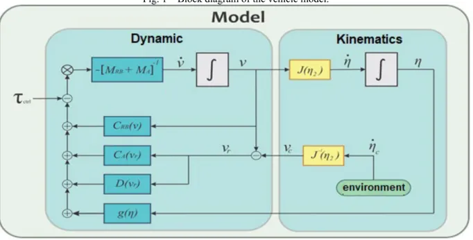
Fig. 1 – Block diagram of the vehicle model.

The vector with the control inputs τ is defined as 𝜏𝜏 = [ 𝑛𝑛, 0, 𝛿𝛿𝑟𝑟], where 𝛿𝛿𝑟𝑟 is the steering

rudder control signal and n the amount of rpm to keep the vehicle at a constant speed and equal to 1 m/s.

In this project, besides considering the constant speed, the depth will also be constant, neglecting the command signal for the vertical rudder. Fig.1 shows the block diagram of the vehicle

model where it is possible to observe both the dynamics and the kinematic equations defined in equations (5) and (6).

Dynamic Model of Darpa ML02

Considering the uncoupled movement, as they did (Healey et al. 1993, Healey and Marco 1992, Jalving 1994), the states of interest for the steering system will be v, r e 𝜓𝜓. Considering also that the vehicle has neutral buoyancy, two planes of symmetry and navigates at low speed (1 m/s), equation (5) can be rewritten as

(5)

Braz. J. of Develop.,Curitiba, v. 6, n. 8, p. 54694-54707 aug. 2020. ISSN 2525-8761 Rearranging the terms in the form of an equation of states, we have, therefore:

The added mass coefficients were calculated according to the strip theory, considering the approximation by a prolate spheroid (Imlay 1961). The moment of inertia was modeled considering the hull a solid cylinder. By replacing the numerical values for the AUV (Table 1), considering 𝑢𝑢𝑜𝑜 = 1 𝑚𝑚/𝑠𝑠, the dynamic model in the form of a state equation results in

Thus, the model presented will be used to describe the dynamics of the vehicle, providing support to the control project of steering autopilot, aiming at tracking the expected trajectories.

3 CONTROL DESIGN

This control technique requires the design of a state space error sliding surface, thus ensuring overall system stability. The state error vector is defined as:

Using 𝑥𝑥�, the sliding hyperplane can be defined by:

Where S1, S2 and S3 are the constants of the sliding surface. The tracking problem boils down to making 𝑠𝑠(𝑥𝑥, 𝑡𝑡) = 0. To ensure trajectory tracking, S will be chosen to ensure that

lim

𝑡𝑡→∞𝑥𝑥� = 0, in other words, that it has asymptotic stability for origin. Taking the function, positive

(6)

It is possible to guarantee that the error states will converge on the sliding surface, provided that

Consider the AUV Darpa ML02 Single-Input Multistate linear model for the direction plane written in the form

Where 𝑓𝑓(𝑥𝑥) describes the linearity deviation in terms of disturbances and unmodelled dynamics. The control law consists of two parts

Where k is the feedback gain vector and 𝑢𝑢𝑜𝑜 the non-linear control law. Replacing u in (15)

For the particular case of 𝑉𝑉̇(𝜎𝜎) = −𝜂𝜂. 𝑠𝑠𝑠𝑠𝑠𝑠𝑛𝑛(𝜎𝜎), where 𝜂𝜂 > 0, differentiating (9) we have to

Assuming that (𝑆𝑆𝑇𝑇_𝑏𝑏)−1_{≠ 0, the control law 𝑢𝑢}

(7)

where 𝑓𝑓̂(𝑥𝑥) is the estimated value of 𝑓𝑓(𝑥𝑥). Thus, the dynamics of 𝜎𝜎 can be written as

where Δ𝑓𝑓(𝑥𝑥) = 𝑓𝑓(𝑥𝑥) − 𝑓𝑓̂(𝑥𝑥). Choosing the coefficients of 𝑆𝑆𝑇𝑇_{as the right eigenvector of 𝐴𝐴} 𝑐𝑐 𝑇𝑇_,

it is possible to cancel the term 𝑆𝑆𝑇𝑇_𝐴𝐴

𝑐𝑐𝑥𝑥, results in

Deriving Lyapunov's candidate function with respect to time

Thus the dynamic of 𝜎𝜎 will be asymptotically stable since

By choosing 𝜂𝜂 so that (18) is negative defined, the Barbalat Lemma ensures that 𝜎𝜎 converges to zero in a finite time if 𝜂𝜂 is chosen to be large enough to overcome the destabilizing effects of unmodelled dynamics Δ𝑓𝑓(𝑥𝑥). The gain 𝜂𝜂 will be the adjustment factor between robustness and trajectory tracking performance (Fossen 1994).

The classic LOS (Line of Sight) method was adopted for guidance of the vehicle. The system receives the desired position [𝑥𝑥𝑑𝑑, 𝑦𝑦𝑑𝑑] from the waypoint database that compose the path. From the

position error the steering angle is calculated by:

The switching of the next waypoint occurs when the vehicle enters the area of the radius acceptance circle R, defined by: (Jalving 1994)

(8)

Braz. J. of Develop.,Curitiba, v. 6, n. 8, p. 54694-54707 aug. 2020. ISSN 2525-8761 The reference path was generated by cubic interpolation methods to link all the points.

4 SIMULATIONS

If the pair (𝐴𝐴, 𝑏𝑏) is controllable and (𝑆𝑆𝑇𝑇_𝑏𝑏)−1 _{≠ 0, então then it is possible to use the classical}

control design for the computation of 𝑘𝑘𝑇𝑇_{(DeCarlo et al. 1988).}

The desired poles were chosen as 𝑃𝑃 = [−4.6, −1, 0]. Using the pole allocation method for calculating the 𝑘𝑘𝑇𝑇_{, the closed loop dynamics, considering (10), we have}

resulting in the closed loop matrix

(9)

Selecting the autovector associated with 𝜆𝜆 = 0 will result in

Thus, considering 𝑣𝑣𝑑𝑑 = 𝑟𝑟𝑑𝑑 = 0 and deriving σ, we will have

Leaving aside 𝜓𝜓̇𝑑𝑑 and including discontinuous entry by making 𝜎𝜎̇ = −𝜂𝜂𝑠𝑠𝑠𝑠𝑠𝑠𝑛𝑛(𝜎𝜎), the control

law results in

Equation (29) thus defines the input signal for control of the Darpa Suboff ML02 vertical rudder, taking into account the vehicle coefficients and parameters listed in Table 1. Finally, replacing all terms found in equation (16), the control law is given by

The model developed in Simulink can be seen in Fig. 1. For trajectory tracking, the LOS

guidance law was implemented so that 𝜓𝜓𝑑𝑑 is defined according to equation (24). The results of the

simulations for trajectory tracking in closed loop, considering model (10) and control law (30), can be seen in Fig. 3. For the smoothing of the overswitched control signal the function 𝑠𝑠𝑠𝑠𝑠𝑠𝑛𝑛(𝜎𝜎) was

replaced by the function 𝑡𝑡𝑡𝑡𝑛𝑛ℎ(𝜎𝜎/Φ), where 𝜂𝜂 = 0.7 and Φ = 0.8.

The speed measurements are described in relation to the fixed body reference. In order to compare the tracking of the vehicle with the reference trajectories it is necessary to transform them into the navigational reference. The output signals (𝑢𝑢, 𝑣𝑣, 𝜓𝜓) in the dynamic model are used to calculate the kinematic equations using the [N,E] module shown in Fig.2, and are defined by

(10)

Where 𝑉𝑉𝑥𝑥 e 𝑉𝑉𝑦𝑦 represent the speeds of the currents that can be inserted in the simulations.

Integrating the values of 𝑥𝑥̇ e 𝑦𝑦̇ and adding to the initial coordinates, the vehicle's current position is obtained in relation

Fig. 3 – Tracking of trajectories 1-4 in closed loop.

to a navigation coordinate system. The guide loop for trajectory tracking is closed with the feedback of the current positions of 𝑥𝑥(𝑡𝑡) e 𝑦𝑦(𝑡𝑡) from the [N,E] module.

Fig. 4 shows the simulations with the insertion of sea currents, according to the orientation

represented by the arrows in each graph. The estimated position of the vehicle was simulated by inserting errors peculiar to inertial sensors of an inertial navigation system. A white noise added to a fixed bias was added to each state. The radius of the switching circle considered in this case was 4 m.

(11)

Fig. 4 – Tracking of trajectories including sea currents.

In the figures are observed deviations of trajectory due to the disturbances. It is also possible to notice the controller's action in order to try to keep on the trajectory. The tracking performance is largely due to the guidance strategy adopted when increasing the number of reference points and, consequently, a higher rate of updating the desired steering angle.

It should be noted that the control law does not provide any compensation for the drift angle caused by sea currents. The objective at this point is to test the steering autopilot of the vehicle acting under conditions that may happen in the experimental tests.

5 CONCLUSIONS

In this article, an autonomous underwater vehicle was modeled with 3 degrees of freedom, considering the uncoupled motion and navigating at a constant speed.

The sliding mode control law was successfully implemented for a SIMS system and obtained satisfactory results considering the tracking of the proposed paths. A continuous hyperbolic tangent function was implemented to substitute the signal function as a tool to smoothness the discontinuous control action, thus contributing to a better energy efficiency, avoiding mechanical wear of the movable parts and overheating of the electric and electronic components.

The response of the autopilot steering is satisfactory, even considering the disturbances, parametric uncertainty and unmodelled dynamics. The adoption of the decoupled model for the lateral and longitudinal planes proved to be advantageous, as it makes it possible to work independently on future projects in the implementation of depth or speed control.

(12)

ACKNOWLEDGMENTS

Special thanks are directed to the Military Institute of Engineering and to the research engineers of the Navy Research Institute for their support during the development of this work.

REFERÊNCIAS

NETO WB, MOURA AJS, SILVA RC, OLIVEIRA VG, JUNIOR HCS, JUNIOR RGP AND SBRAGIO R. 2018. Development of a Propeller for an Autonomous Underwater Vehicle with a Hull Geometry of the Darpa Suboff Model, Congresso Nacional de Engenharia Mecânica.

GROVES NC, HUANG TT AND CHANG MS. 1989. Geometric Characteristics of Darpa Suboff Models (DTRC Model 5470 and 5471).

GERTLER M AND HAGEN GR. 1967. Standard Equations of Motion for Submarine Simulation. Technical report, David Taylor Research Center.

AVILA JP. 2008. Modelagem e Identificação de Parâmetros Hidrodinâmicos de um Veículo Robótico Submarino, Tese de Doutorado, Universidade de São Paulo, Brasil.

HEALEY AJ AND LIENARD D. 1993. Multivariable Sliding-Mode Control for Autonomous Diving and Steering of Unmanned Underwater Vehicles, IEEE Journal of Oceanic Engineering, 18(3):327-339.

SFAHANI ZF, VALI A AND BEHNAMGOL V. 2017. Pure Pursuit Guidance and Model Predictive Control of an Autonomous Underwater Vehicle for Cable/Pipeline Tracking, ICCIA, Shiraz, 279-283.

YANGYANG Z, LI'E G, WEIDONG L AND LE L. 2017. Research on Control Method of Auv Terminal Sliding Mode Variable Structure, International Conference on Robotics and Automation Sciences, ICRAS 2017, 88-93.

YAN Y AND YU S. 2018. Sliding Mode Tracking Control of Autonomous Underwater Vehicles with the Effect of Quantization, Ocean Engineering, 151:322-328.

XIA Y, XU K, LI Y, XIANG X, XU G AND XIANG X. 2019. Improved Line-Of-Sight Trajectory Tracking Control of Under-Actuated AUV Subjects to Ocean Currents and Input Saturation, Ocean Engineering, 174:14-30.

XINGHUA C AND LUAN L. 2014. AUV Planner Tracking Control Based on the Line of Sight Guidance Method, IEEE International Conference on Mechatronics and Automation, IEEE ICMA 2014, Tianjin, 1204-1208.

FOSSEN TI, BREIVIK M AND SKJETNE R. 2003. Line-of-Sight Path Following of Underactuated Marine Craft, IFAC Proceedings Volumes, 36(21):211-216.

(13)

LUQUE JCC AND DONHA DC. 2008. AUV Robust Guidance Control, IFAC Proceedings Volumes, 41(1):85-90.

ATAEI M AND YOUSE-KOMA A. 2015. Threedimensional Optimal Path Planning for Waypoint Guidance of an Autonomous Underwater Vehicle, Robotics and Autonomous Systems, 67:23-32. FOSSEN TI. 1994. Guidance and Control of Ocean Vehicles, John Wiley & Sons.

SNAME – SOCIETY OF NAVAL ARCHITECTS AND MARINE ENGINEERS. 1950. Nomenclature for Treating the Motion of a Submerged Body Through a Fluid, Report of the American Towing Tank Conference.

FOSSEN TI. 2011. Handbook of Marine Craft Hydrodynamics and Motion Control, 1st ed, John Wiley & Sons.

HEALEY AJ AND MARCO DB. 1992. Slow Speed Flight Control of Autonomous Underwater Vehicles: Experimental Results with NPS AUV II, The Second International Offshore and Polar Engineering Conference, 14-19.

JALVING B. 1994. The NDRE-AUV Flight Control System, IEEE Journal of Oceanic Engineering, 19(4):497-501.

IMLAY FH. 1961. The Complete Expressions for Added Mass of a Rigid Body Moving in an Ideal Fluid, Technical report, David Taylor Research Center.

BANDYOPADHYAY B, JANARDHANAN S AND SPURGEON SK. 2013. Advances in Sliding Mode Control, volume 440.

DECARLO RA, ZAK SH, MATTHEWS GP. 1988. Variable Structure Control of Nonlinear Multivariate Systems: A Tutorial, Proceedings of the IEEE, 76(3):212-232.

PETTERSEN K AND EGELAND O. 1999. Time-Varying Exponential Stabilization of the Position and Attitude of an Underactuated Autonomous Underwater Vehicle, IEEE Transactions on Automatic Control, 44(1):112-115.

(14)

APPENDIX

TABLE 1- Model Parameter.

Description Notation Value

Length (m) L 2.743 Maximum radius (m) R 0.16 Moment of Inertia1 (Kg.m2₎ 𝐼𝐼𝑥𝑥 2.26 𝐼𝐼𝑦𝑦 112.11 𝐼𝐼𝑧𝑧 112.11 Added mass coefficients2 𝑋𝑋𝑢𝑢̇ -4.65 𝑌𝑌𝑣𝑣̇ -168.15 𝑁𝑁𝑟𝑟̇ -47.72 Linear Damping Coefficients 𝑋𝑋𝑢𝑢 -15 𝑌𝑌𝑣𝑣 -100 𝑁𝑁𝑟𝑟 -30

Steering wheel damping coefficients

𝑌𝑌𝛿𝛿𝑟𝑟 286.61 𝑁𝑁𝛿𝛿𝑟𝑟 -48.74

Resources: (Neto et al. 2018, Healey et al. 1993,

Pettersen and Egeland, 1999).

Notes: 1_{For the calculation of the inertia matrix, the} symmetry plans of the hull modeling as a massive cylinder were considered.

2 _{The added mass coefficients were calculated}

according to the strip theory by modeling the hull by a prolato spheroid (Fossen 1994).