Optimal District Metered Area Design by Simulated Annealing

Optimal District Metered Area design by

Simulated Annealing

Ricardo Gomes

1,5*

_{, Joaquim Sousa}

2,5

_{, Alfeu Sá Marques}

2,5

_{and João}

Muranho

4,5

1 _{Polytechnic Institute of Leiria, School of Technology and Management, Leiria, Portugal} 2 _{Polytechnic Institute of Coimbra, Department of Civil Engineering, Coimbra, Portugal}

3 _{University of Coimbra, Department of Civil Engineering, Coimbra, Portugal} 4 _{University of Beira Interior, Department of Computer Science, Covilhã, Portugal} 5 _{INESC Coimbra – Institute for Systems Engineering and Computers at Coimbra, Portugal}

ricardo.gomes@ipleiria.pt, jjoseng@isec.pt, jasm@dec.uc.pt, jmuranho@ubi.pt

Abstract

Water losses reduction in Water Distribution Systems (WDSs) is nowadays an issue of growing importance for water companies to ensure the economic sustainability of these public services. In this context, the implementation of District Metered Areas (DMAs) and/or pressure management are considered effective tools for leakage control, particularly in large networks and in systems with deteriorated infrastructures and with high pressure.

Based in previous studies performed by the authors (Gomes et al., 2012; Gomes et al., 2015; Sousa et al., 2015), the methodology described in this paper follows the ‘water losses management international best practices’ and makes it possible to evaluate the Net Present Value (NPV) of DMAs project, as well as the benefits that can be achieved by pressure management in WDS, particularly in terms of water production reduction. Leakage assessment is performed using the analysis of the minimum night flow and the FAVAD concept, and it uses a pressure driven simulation model to predict the network hydraulic behaviour under different pressure conditions. The optimal location of DMAs entry points, pipes reinforcement/replacement and locations/settings of the Pressure Reduction Valves (PRVs) are identified by a Simulated Annealing algorithm. The potential of this methodology is illustrated through an hypothetical case study.

* _{Corresponding author.}

HIC 2018. 13th International Conference on Hydroinformatics

1 Introduction

Water Distribution Systems (WDSs) consist of a complex networks of pipes and fittings, pumps, valves and storage tanks, subjected to different loads (water demand and demand pattern) and operating rules. The complexity of the WDSs management has been increasing significantly over the last decades (because of the expansion of urban areas and water infrastructures degradation) and nowadays new technologies for continuous monitoring are imperative to ensure good service levels over a given planning period. On the other hand, once the economic funding is limited, each intervention in WDSs must be duly weighted in order to obtain the highest return of investment and, for that reason, new tools to support decision makers' are required also.

Several studies show that residential water demand makes up the majority of water use in urban WDSs but the flow varies over time (hour, day, month or year) depending on the number of customers, water cost, level of water losses, season of the year, the level of economic development and water uses and the efficiency in the water use. In this context, to guarantee high levels of performance, the appropriate water infrastructure planning and management requires reasonable water demand forecasts for the future years, as well as the knowledge of the network hydraulic behaviour, degradation of infrastructures and the need for network expansion. However, recently water loss control has been an issue of growing importance to ensure the economic sustainability of these public services and, for that reason, greater efforts are being made in this direction in several water companies worldwide.

The implementation of DMAs and/or pressure management are considered effective tools for leakage control, particularly in large networks and in systems with deteriorated infrastructures and with high pressure. The size of each DMA and the optimal DMA entry points vary from system to system, and depend on the network configuration, the infrastructure condition, the water quality and the financial resources of the water companies. The experience demonstrates that in urban areas the adequate size for a DMA should be between 500 and 3,000 service connections, but it can be reduced to 500 to 1,000 in deteriorated infrastructures. By no means should be advisable to have a DMA containing more than 5,000 service connections, because it gets too difficult to control water losses (location of new leaks can become extremely demanding). Alternatively, in areas with low density of service connections, the size of a DMA should be fixed in terms of pipe length, because the difficulty to find leaks is more related to the pipe length than to the number of service connections. Each DMA should be supplied by a limited number of pipes in which flow meters are installed (entry points), to measure water imports (if a DMA supplies other DMAs, they also measure water exports), and these are not to be necessarily definitive because changes in the operating conditions may imply modifying the boundaries. There are many examples of success worldwide on implementation of DMAs (Thornton et al., 2008). Furthermore, several models have been developed to illustrate the cost and economic benefit of DMAs management in practice (WRc, 1994; Morrison et al., 2007).

The methodology described in this paper follows the ‘water losses management international best practices’ and makes it possible to evaluate the Net Present Value (NPV) of DMAs project, as well as the benefits that can be achieved by pressure management in WDSs, particularly in terms of water production reduction. Leakage assessment is performed using the analysis of the minimum night flow and the FAVAD concept, and it uses a pressure driven simulation model to predict the network hydraulic behaviour under different pressure conditions. The optimal location of DMAs entry points, pipes reinforcement/replacement and locations/settings of the Pressure Reduction Valves (PRVs) are identified by a Simulated Annealing algorithm (Kirkpatrick et al., 1983). The potential of this methodology is illustrated through an hypothetical case study.

2 Methodology

The DMAs design can be formulated as an optimization problem. This NP-hard problem is related to the number of DMAs and the total number of DMAs entry points (flow meters), the pipes to reinforce/replace and the most advantageous type, location and settings for the PRVs. The objective function NPV(X) maximizes the NPV of the differences between the economic benefits from pressure management (reduction of water production cost minus the reduction of revenue from billed water) and the total implementation costs (flow meters, PRVs, chambers and pipes reinforcement/replacement), for a given planning period, equations (1) to (3). However, additional costs and benefits can be included in this methodology.

(1)

(2) (3)

where: NPV(X) is the objective function or NPV of the project (€); X is the solution of the Simulated Annealing algorithm; n is the number of investment periods along the duration of the project plan;

B(X)i is the total economic benefits during the investment period i and updated to the beginning of

this investment period (€); C(X)i is the total investment costs at the beginning of the investment period

i (€); πi is the time from the beginning of the project to the investment period i (years); intR is the

annual interest rate (%); NP is the number of pipes; Cpipe,p(Dp) is the unit cost for the pipes

reinforcement/replacement (€/m); Dp is the diameter of the new pipe (mm); Lp is the pipe length (m);

NM is the number of DMAs entry points; Cinlet,m(DFm) is the global cost of each DMA entry point

with flow meter and chamber (€/unit); DFm is the flow meter diameter (mm); Cinlet,m(DPRVm) is the

global cost of the PRV at each DMA entry point (€/unit); DPRVm is the PRV diameter (mm); NV is

the number of constraints violations (hydraulics behaviour or operational constraint); violv is the maximum violation for the constraint v; βv is the unit cost of penalty for violating constraint v; ny is the duration of each investment period (years); Cp is the cost of water production (€/m3); Cv is the

water selling price (€/m3_{); ΔVL is the total reduction of water losses after pressure management (m}3_); and ΔVR is the total reduction of billed water after pressure management (m3_).

Simulated annealing is a probabilistic method proposed initially by Kirkpatrick et al. (1983) for finding the global minimum of a cost function that may possess several local minima. Table 1 shows the cooling scheme adopted for the Simulated Annealing algorithm. At the initial temperature (T0), the algorithm starts by generating an initial solution (X0), which corresponds: i) the biggest diameter is assigned to each pipe in the network; ii) each pipe between DMAs is an entry point (there are no boundary valves); iii) the location and adjustment of PRVs will be defined later, when the hydraulic behaviour is checked. At temperature Tk+1 the number of solutions generated is Lk+1, which varies according to the percentage of solutions accepted at the last temperature (Pak). Each new solution (Xz) is generated from the current solution (Xz-1) by randomly applying one of the following procedures: 1) select a DMA and reduce/increase its number of entry points; 2) select a DMA and change one of its entry points; or 3) select one of the investment periods and change a pipe diameter (in 60% of the

( )

(

)

maximum 1 1 p = -= +

å

i n i i i B( X ) C( X ) NPV X int R

( )

( )

(

)

(

)

(

)

1 1 1

b

= = =

é

ù

=

å

NP

_ë

_{pipe,p p}

´

_p

_û

+

å

NM

_ë

é

_{inlet ,m m}

+

_{inlet ,m m}

_û

ù +

å

NV _v

´

_v

p m v

C X

C

D

L

C

DF

C

DPRV

viol

(

)

365

(

1

₍

)

1

₎

1 é _{+ -} ù é ù =_ë ´ D - - ´ D _û´ê ´ ú ´ + ê ú ë û ny p v p ny int R B( X ) C VL C C VR int R int R

cases the diameter is reduced – this procedure allows improving the performance of the algorithm and accelerates its convergence). For each solution, a pressure driven simulation model is used to predict the network hydraulic behaviour under different pressure conditions and equation (1) is used to evaluate the NPV for the new solution. The costs and the total economic benefits for each investment period are estimated using equations (2) and (3), respectively. The new solution is accepted or not, according to the Metropolis criterion. If it is accepted, this solution will be used as the starting point for the next step. If not, the original current solution will be used. The algorithm ends if the stop criterion is reached, that is: for two successive temperatures the number of solutions accepted (Pak) remains lower than 5% and the difference between the averages of the project NPV between two successive temperatures is 1.0% (ε) or lower.

Initial configuration

Initial temperature

Cooling scheme

Stop criterion

Table 1: Cooling scheme for the Simulated Annealing algorithm

3 Case study

3.1 Water Distribution System data

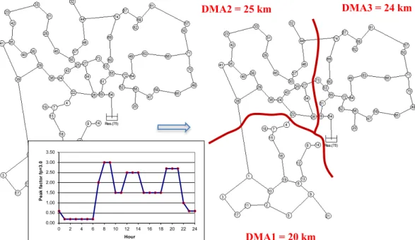
Figure 1 (left) shows the layout and average daily pattern demand of the WDS. The network has 69 km (84 pipes and 75 nodes) and is characterized by low density of service connections – the density of service connection throughout of the network is proportional to the average demand in each node. The pipe material is Polyvinyl Chloride (diameters from 90 mm to 400 mm) and the network ground elevation changes between 985 m and 1022 m. The study area is gravity-fed from a single tank (ground elevation 1064 m) and the network ensures the water distribution service to 12,000 inhabitants (6,000 service connections). The average daily demand at the system entry point is 99.97 m3_{/h (200} litres/inhabitant/day) and the percentage of water losses is 40%. It is considered that whole authorized consumption is measured and billed and the population remains constant over the planning period. The minimum and maximum service pressures are 39.96 m (node 54) and 77.49 m (node 23), respectively. The minimum pressure required to ensure the demand over the planning period is 18.37 m (which represents two floors above ground level, including ground floor).

{

D ,D ,...,D

}

D ; where:NP numberofnetworkpipes X0= 1 2 NP = max

( )

( )

Pa ; where:Pa 80% ln X NPV 0.10 T 0 0 0 0 _÷÷ = ø ö çç è æ ´ -= NP 75 L and T 0.95 T then 20% Pa if NP 75 L and T 0.90 T then 50% Pa 20% if NP 50 L and T 0.75 T then 80% Pa 50% if NP 20 L and T 0.50 T then 80% Pa if 1 k k 1 k k 1 k k 1 k k 1 k k 1 k k 1 k k 1 k k ´ = ´ = £ ´ = ´ = £ < ´ = ´ = £ < ´ = ´ = > + + + + + + + + NPV NPV -NPV ε : with 1.0% ε 5% Pa 1 k average, 1 k average, k average, k + + = £ < 813

Figure 1 (right) shows the area proposed for each DMA (right), where the pipe length was used as a criterion to define the area of each DMA. In the DMAs project the greatest problem is related to the optimal number/location of DMAs entry points, especially when there are different options to consider. Previews studies recommend one entry point for each DMA, and this was the criterion used in this case study. Three types of PRVs were considered for pressure management – based on the maximum pressure adjustment at the DMAs entry points over the period time considered: i) Fixed-outlet PRV (ΔP ≤ 10 m); ii) Time-modulated PRV (10 m < ΔP ≤ 20 m); iii) Pressure-modulated PRV (ΔP > 20 m). The minimum pressure adjustment at DMA entry point shall not be less than 3.0 m. For the NPV project, it is assumed that prices remain constant over time, and an annual interest rate of 5%. Over the planning period, the increase of daily water demand and infrastructure degradation was considered constant (1.25%/year and 1.0%/year, respectively). The cost of producing and selling water is considered equal to 0.5 €/m3 _{and 1.25 €/m}3_{, respectively.}

Figure 1: Water Distribution System layout (left) and the area proposed for each DMA (right).

3.2 Optimal solution for DMAs design

Using the methodology describe in section 2, three scenarios were proposed in order to evaluate the NPV of the DMAs design, that include the identification of optimal DMAs entry point, the pipes reinforcement/replacement and the benefits from pressure management (see Tables 2 and 3). For Scenario 1, the DMAs design should be driven by network hydraulic behaviour (each DMA entry point should include only a flow meter – FM). For Scenario 2, the DMAs design should be driven to obtain the maximum benefits from pressure management (each DMA entry point should include a FM and, when advantageous, a PRV). For Scenario 3, the DMAs design should be driven to obtain the maximum benefits from pressure management, including the advantage on the hydraulic behaviour after network reinforcement/replacement (each DMA entry point should include a FM and, when advantageous, a PRV and pipe reinforcement/replacement).

1.50 2.00 2.50 3.00 3.50 Pe a k f a c to r fp = 3 .0 DMA3 = 24 km DMA2 = 25 km DMA1 = 20 km 0.00 0.50 1.00 1.50 2.00 2.50 3.00 3.50 0 2 4 6 8 10 12 14 16 18 20 22 24 Pe a k f a c to r fp = 3 .0 Hour 814

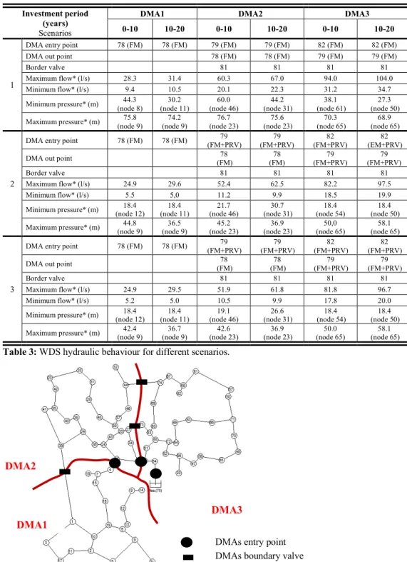
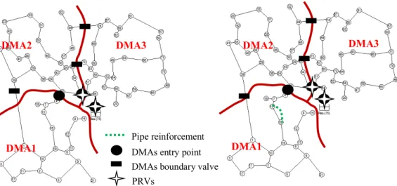
Tables 2 and 3 show (respectively) the NPV of the DMAs design and the hydraulic behaviour of the WDS, for each scenario. For Scenario 1, the value of NPV obtained was -29,076 € and it is associated with the cost of the flow metering stations. The benefit from pressure management is a consequence of the installation of the DMAs boundary valves, which changes the service pressure in the WDS. Additionally, the DMAs are arranged in series, that means DMA1 is supplied from DMA2, DMA2 from DMA3, and DMA3 is fed directly from the tank at the WDS entry point. When analysing the service pressure throughout the network, it is checked that the minimum service pressure is still very high (>> 18.37 m) so, for Scenario 2 an additional benefit was calculated due to the advantage of pressure management at the DMAs entry points (the NPV of the DMAs design improved to 2,041,446 €). Taking as reference the NPV obtained from Scenarios 1 and 2, it is possible to demonstrate that the economic viability of the project is related to the benefits from pressure management throughout the network. Two types of PRVs have been selected over the planning period: i) for 1st Investment period (0-10) 2 Fixed-outlet PRV are required at each DMA2 and DMA3 entry points; ii) for 2nd Investment period (10-20) it is required one Fixed-outlet PRV at DMA2 entry point and one Pressure-modulated PRV at DMA3 entry point. Regarding Scenario 3, results show that the network reinforcement at the beginning of the planning period (pipe 18; diameter 200 mm) allows a readjustment of the service pressures throughout the network and, consequently, increase the NPV by 0.5% (NPV changes to 2,051,658 €). In this scenario the positions and types of PRVs are the same from scenario 2 but the operating conditions are different. Figures 2 and 3 show for each scenario the optimal locations for FM stations, boundary valves and PRVs at the DMAs entry points, as well as the pipe reinforcement. For Scenarios 2 and 3 two pressure zones are proposed: the first pressure zone includes DMA1 and DMA2, and the second pressure zone includes DMA3.

Investme nt period (years) Scenarios Average daily reduction* (%)

DMA entry point

Cost of network reinforcement or replacement (€) Cost of flow meter and PRV (€) Benefits (€) NPV (€) Billed

volume Water losses

1 0-10 0.00 0.02 DMA1–pipe 78 (FM) DMA2–pipe 79 (FM) DMA3–pipe 82 (FM) 0 -31,391 3,238 -29,076 10-20 0.00 0.03 DMA1–pipe 78 (FM) DMA2–pipe 79 (FM) DMA3–pipe 82 (FM) 0 -7,154 5,650 2 0-10 1.32 12.87 DMA1–pipe 78 (FM) DMA2–pipe 79 (FM + PRV) DMA3–pipe 82 (FM + PRV) 0 -39,582 1,308,645 2,041,446 10-20 1.07 11.18 DMA2–pipe 79 (FM + PRV) DMA1–pipe 78 (FM) DMA3–pipe 82 (FM + PRV) 0 -7,072 1,265,202 3 0-10 1.40 13.64 DMA1–pipe 78 (FM) DMA2–pipe 79 (FM + PRV) DMA3–pipe 82 (FM + PRV) -66,684 -39,582 1,371,470 2,051,658 10-20 1.08 11.44 DMA1–pipe 78 (FM) DMA2–pipe 79 (FM + PRV) DMA3–pipe 82 (FM + PRV) 0 -7,072 1,288,123

Table 2: NPV of the DMAs project for different scenarios.

Investment period (years)

Scenarios

DMA1 DMA2 DMA3

0-10 10-20 0-10 10-20 0-10 10-20

1

DMA entry point 78 (FM) 78 (FM) 79 (FM) 79 (FM) 82 (FM) 82 (FM)

DMA out point 78 (FM) 78 (FM) 79 (FM) 79 (FM)

Border valve 81 81 81 81

Maximum flow* (l/s) 28.3 31.4 60.3 67.0 94.0 104.0

Minimum flow* (l/s) 9.4 10.5 20.1 22.3 31.2 34.7

Minimum pressure* (m) _{(node 8)} 44.3 _{(node 11)} 30.2 _{(node 46)} 60.0 _{(node 31)} 44.2 _{(node 61)} 38.1 _{(node 50)} 27.3 Maximum pressure* (m) _{(node 9)} 75.8 _{(node 9)} 74.2 _{(node 23)} 76.7 _{(node 23)} 75.6 _{(node 65)} 70.3 _{(node 65)} 68.9

2

DMA entry point 78 (FM) 78 (FM) 79

(FM+PRV) 79 (FM+PRV) 82 (FM+PRV) 82 (EM+PRV)

DMA out point _(FM) 78 _(FM) 78 _(FM+PRV) 79 _(FM+PRV) 79

Border valve 81 81 81 81

Maximum flow* (l/s) 24.9 29.6 52.4 62.5 82.2 97.5

Minimum flow* (l/s) 5.5 5,0 11.2 9.9 18.5 19.9

Minimum pressure* (m) _{(node 12)} 18.4 _{(node 11)} 18.4 _{(node 46)} 21.7 _{(node 31)} 30.7 _{(node 54)} 18.4 _{(node 50)} 18.4 Maximum pressure* (m) _{(node 9)} 44.8 _{(node 9)} 36.5 _{(node 23)} 45.2 _{(node 23)} 36.9 _{(node 65)} 50,0 _{(node 65)} 58.1

3

DMA entry point 78 (FM) 78 (FM) 79

(FM+PRV) 79 (FM+PRV) 82 (FM+PRV) 82 (FM+PRV)

DMA out point _(FM) 78 _(FM) 78 _(FM+PRV) 79 _(FM+PRV) 79

Border valve 81 81 81 81

Maximum flow* (l/s) 24.9 29.5 51.9 61.8 81.8 96.7

Minimum flow* (l/s) 5.2 5.0 10.5 9.9 17.8 20.0

Minimum pressure* (m) _{(node 12)} 18.4 _{(node 11)} 18.4 _{(node 46)} 19.1 _{(node 31)} 26.6 _{(node 54)} 18.4 _{(node 50)} 18.4 Maximum pressure* (m) _{(node 9)} 42.4 _{(node 9)} 36.7 _{(node 23)} 42.6 _{(node 23)} 36.9 _{(node 65)} 50.0 _{(node 65)} 58.1

Table 3: WDS hydraulic behaviour for different scenarios.

Figure 2: DMAs design for Scenario1 (NPV = -29,076 €).

DMAs entry point DMAs boundary valve

DMA3 DMA2

Figure 3: DMAs design for Scenario 2 (left, NPV = 2,041,446 €) and Scenario 3 (right, NPV = 2,051,658 €).

4 Conclusions

Water loss reduction in WDSs is nowadays an issue of growing importance for water companies to ensure the sustainability of these public services. On the other hand, reducing water losses to zero is practically impossible and would be extremely expensive. The methodology used in this paper has shown that the DMAs design and pressure management can be used to reduce the total water losses in WDSs and, at the same time, spread the investment cost through the project plan. On the other hand, DMAs design can change significantly the WDS hydraulic behaviour, because of the DMAs boundary valves effect and, sometimes, the network reinforcement/replacement can readjust the service pressure throughout the network and increase de NPV of the DMAs design.

References

Gomes, R., Sá Marques A., Sousa, J. (2012). Decision support system to divide a large network into suitable District Metered Areas. Water Science & Technology, IWA Publishing, 65(9), 1667-1675.

Gomes, R., Sousa, J., Muranho, J., Sá Marques (2015). Different design criteria for district metered areas in water distribution networks. In Proceedings of the 13th International Conference on

Computing and Control for the Water Industry – CCWI 2015, Vol. 119 1221–1230.

Kirkpatrick, N., Gelatt Jr., S., Vecchi, M. P. (1983). Optimization by simulated annealing. Science 220(4598): 671-680.

Morrison, J., Tooms, S., Rogers, D. (2007). District Metered Areas, Guidance Notes. IWA Water

Loss Task Force, Specialist Group on Efficient Operation and Management of Urban Water

Distribution Systems.

Sousa, J., Muranho, J., Sá Marques, A., Gomes, R. (2015). Optimal management of water distribution networks with simulated annealing: The C-Town problem. Journal of Water Resources

Planning and Management, 142(5), C4015010.

Thornton, J., Sturm, R., Kunkel, G. (1994). Water Loss Control. McGraw-Hill Companies, 2008. WRc, Managing Leakage Reports A-J. Swindon (UK), UK Water Industry Research Ltd/Water Research Centre.

DMAs entry point DMAs boundary valve PRVs Pipereinforcement 0.00 0.50 1.00 1.50 2.00 2.50 3.00 3.50 0 2 4 6 8 10 12 14 16 18 20 22 24 Pe a k f a c to r fp = 3 .0 Hour DMA1 DMA3 DMA2 DMA1 DMA2 DMA3 817