MASTER IN
ACTUARIAL SCIENCE
M
ASTER
F
INAL
W
ORK
INTERNSHIP REPORT
IMPACT OF A LONGEVITY SWAP
ON A UK PENSION SCHEME
JOÃO MANUEL DE AGUIAR MORAIS DE MATOS
MASTER IN
ACTUARIAL SCIENCE
M
ASTER
F
INAL
W
ORK
INTERNSHIP REPORT
IMPACT OF A LONGEVITY SWAP
ON A UK PENSION SCHEME
JOÃO MANUEL DE AGUIAR MORAIS DE MATOS
SUPERVISION
ELIZABETH
METCALFE
ONOFRE
ALVES
SIMÕES
I
List of figures
1. Deaths per 100.000 population in England and Wales between 2001 and
2018. ……….………..………..………..………..………. 24 2. Expected cash flows for the members that were covered by the longevity
Swap. ………..………..… 27 3. Comparison between the expected cash flows………..…..………... 28
II
List of tables
Table 1 - Mortality tables published by the CMI. ………..……… 21 Table 2 – Mortality assumptions agreed between the scheme and the insurer. …….……….. 26 Table 3 - Estimated cashflows for the three years between 2013 and 2016……….. 32 Table 4 - September RPI. ……… 32
III
Abstract
Managers of pension funds in the UK are more and more concerned about the losses that might result from the majority of the members of the schemes living longer than expected. Providentially, to assist them in handling the problem, there is a panoply of actuarial and financial products designed to prevent the schemes from having very high losses, or even becoming insolvent. One of these products (and the main topic of this work) is the Longevity Swap.
This report was developed in the sequence of a curricular internship at the Lisbon office of Willis Towers Watson. The principal work developed during the internship was directly related to valuing the liabilities of pension funds.
Although the tasks I performed during the internship were not directly related to longevity swaps, this issue really caught my interest. This happened because not only longevity risk is a pressing problem for pension funds, and as such is extremely worrying, but also because it was a topic studied during the master’s course, so it was very interesting to be able to cross this bridge.
Moreover, the study of a real case, allowed me to better understand how pension funds work in the UK. This proved to be very important, as funds in the UK, due to the complexity of some of them, have a very particular way of functioning.
IV
Resumo
No reino Unido, os gestores de fundos de pensões estão cada vez mais preocupados com as perdas que podem advir do facto de a maioria dos membros dos esquemas que gerem viverem mais do que o esperado. Providencialmente, para os ajudar a lidar com o problema, existe uma panóplia de produtos atuariais e financeiros, projetados para impedir que os fundos sofram perdas demasiado elevadas, que os possam inclusivamente levar à insolvência. Um desses produtos (e o principal tópico deste trabalho) é o chamado Swap de Longevidade.
Este relatório foi desenvolvido na sequência de um estágio curricular no escritório da Willis Towers Watson, em Lisboa. O principal trabalho desenvolvido durante o estágio esteve diretamente relacionado com a avaliação das responsabilidades dos fundos de pensão. Embora as tarefas desempenhadas durante o estágio não estivessem de forma explícita ligadas aos Swaps de Longevidade, o tema pareceu realmente interessante, não só porque o risco de longevidade é um problema premente para os fundos de pensões e, como tal, é extremamente preocupante, mas também porque foi um tópico estudado durante o curso de mestrado. Assim, foi muito motivador estabelecer essa ponte.
Adicionalmente, o estudo de um caso real possibilitou uma melhor compreensão do modo como os fundos de pensão funcionam no Reino Unido. Isso provou ser muito importante, uma vez que, devido à complexidade de alguns deles, os fundos no Reino Unido têm uma maneira muito particular de funcionar.
Palavras-chave: Planos e fundos de Pensões, Risco de Longevidade, Swap de Longevidade, Reino Unido
V
Acknowledgements
I would like to appreciate my gratitude to my mother who is my greatest supporter and believer, who knows my abilities more than myself and that always tries to push me forward.
I would also like to thank my family and friends, who have been very patient with me throughout this process, who always gave me words of encouragement and were always interested to know my progress in this work.
To Arta, Elena, Gracinha, Haliyah and Patrícia for being my company on the nights and weekends I stayed at work doing this report, for being my motivation and for providing support and advice when needed.
To my closest friends, who have never left my side, Alexandra, Rute, Catarina and Isa for their understanding and to my new friends, that I had the opportunity to meet at Willis Towers Watson, especially Sudharshan for his help.
A very special thanks to my line manager Patricia Canavezes, for her motivation and care. To Elizabeth Metcalfe, thank you for all your help during this work, for putting me in contact with consultants and for your understanding, for always making time, for not giving up on me and for your care in making sure that this work was according to standards.
To Onofre Alves Simões, it has been a long path and I’m glad I could finish my Master’s with you by my side. Thank you for your care, for your patience, for you faith, for your motivation. It was my pleasure working with you.
I would also like to thank Willis Towers Watson for the opportunities they gave me, for everything I got to learn and for giving me the means to develop this work.
VI
Contents
List of figures I List of tables II Abstract III Resumo IV Acknowledgements V 1. Introduction 12. Pension Funds Basics 3
2.1. Pension Schemes... 3
2.1.1. Occupational Pension Schemes 3 2.2. Valuations ... 5
2.2.1. Statutory funding objective (SFO) 6 2.2.2. PPF buy-out/section 179 measure 7 2.2.3. Self-sufficiency 7 2.2.4. Insurance buy-out 8 2.2.5. Accounting valuation 8 3. Risks for Defined Benefit Schemes 10 3.1. Longevity Risk ... 10
3.2. Interest Rate Risk ... 11
3.3. Inflation Rate Risk ... 11
3.4. De-risking techniques through the purchasing of annuities ... 12
3.4.1. Buy-in/ buy-out 12 3.4.2. Longevity Swaps 12 4. Mortality Assumptions 20 4.1. CMI standard mortality tables ... 20
4.2. CMI Mortality Improvements tables ... 22
5. Application of a Longevity Swap on a Real Client 24 5.1. Impact of changing the long-term longevity improvement rate ... 26
5.2. Impact of entering into the contract ... 29
5.2.1. Case 1: Actual mortality lower than expected 29 5.2.2. Case 2: Actual mortality higher than expected 30 5.3. The effect of the premium ... 30
VII
5.4. Actual Experience ... 31 5.4.1. Payments from the scheme 32 5.4.2. Analysis of surpluses and losses 33
6. Conclusion 36
1
1.
Introduction
Pension funds in the UK that have promised many years ago benefits to their members are seeing increasing difficulty in fulfilling those promises given the unfavourable movements in recent years. Though there are more impactful risks to a pension scheme, longevity risk is not one to ignore. For many years, mortality has been slowly decreasing. This poses a risk for pension schemes because an unexpected decrease on mortality will lead to pensions in payment for longer than anticipated. As such, assumptions on mortality improvements are constantly revised to allow for this constant evolution in mortality rates (Swiss Re 2018). It is now important to understand mechanisms that would allow the scheme to deal with the risk of their members living longer than expected. For this purpose, a type of insurance called Longevity Swap has been created. Longevity Swap is one of the mechanisms that allow for de-risking a pension scheme and that solely focuses on longevity risk (Nicholl 2018).
In this report, it will be explained how Longevity Swaps work, how they compare to other de-risking techniques and how they could impact on a pension scheme.
The work was developed as part of an internship agreement at Willis Towers Watson and the topic emerged from a conversation about de-risking pension funds. At a certain point it was suggested that I should do a study on this type of de-risking technique.
Both the internship and the topic chosen for the report made me aware of the dimension of the longevity risk, which was a topic covered in the Master’s Degree course. A case study with a real client greatly contributed to a better understanding of how pension funds work in the UK. In fact, pension funds in this country have a very particular way of functioning, due to the complexity of some of them.
The questions that should be covered in this report are: What are Longevity Swaps? How do they compare to other de-risking techniques? In what way are they beneficial for the scheme?
2 The text has the following structure: Chapter 2 introduces the basics of pension schemes; in chapter 3, we discuss the setting of assumptions on mortality, essential when considering the longevity risk; Chapter 4 contains the application of a longevity swap to a real client; Chapter 5 concludes.
3
2.
Pension Funds Basics
In order to explain what a Pension Fund is, it is important to start by explaining what a Pension Plan (or Pension Scheme) is.
2.1. Pension Schemes
A Pension Scheme is a type of saving scheme aiming to fund benefits to its members after retirement. Each scheme will have a defined set of rules which determines how benefits are managed and calculated. Rules may cover: age retirement, late retirement benefits, disability or death benefits.
A pension scheme is a long term savings plan, where the members make deposits of a part of their regular income, in order to have a source of income when they retire. These deposits are called contributions and they are deposited into a fund. The fund will then invest the money and be responsible to pay the members’ pension upon retirement. There are several types of pension schemes, but the focus will be on occupational pension schemes.
2.1.1. Occupational Pension Schemes
According to (OECD 2005) an Occupational Pension Scheme is a type of plan in which the access is “linked to an employment or professional relationship” between the plan member and the sponsor (the entity that establishes the scheme). Therefore, the plan “may be
administered directly by the plan sponsor or by an independent entity”.
In this type of scheme, the contributions are usually done by both the employer and the employee. Upon retirement, the benefit will depend on which of the following categories of pension schemes is applicable for the members:
• Defined Benefit (DB) schemes; • Defined Contribution (DC) schemes; • Hybrid schemes.
2.1.1.1. Defined Benefit Schemes
Defined Benefit (DB) pension scheme is defined in (EIOPA 2019) as a “retirement plan that
guarantees a specific retirement benefit amount for each scheme member”. This means that
upon retirement, the benefit the member gets is fixed, regardless of the fund’s investment performance.
4 On this type of scheme, the sponsor would bear almost all the risks. This means that on top of the normal contributions that the sponsor makes, additional contributions may also be required to cover deficits for the scheme derived from unexpected events. This is due to the fact that benefits are calculated using a pre-defined formula, with guaranteed increases, that must be met at the time of retirement. If for some reason the fund believes that the benefits are at risk of not being met (due to a low funding position), they would require the sponsor to contribute with additional funds to improve the scheme’s funding position. DB pension schemes have their advantages to the sponsor, especially if the sponsor is the employer, as it can be seen as a reward for the employees due to good service (therefore, a stimulus).
Because Willis Towers Watson only works with Defined Benefit Pension Schemes, we will only be focusing on this type of schemes.
2.1.1.2. Defined Contribution Schemes
In (EIOPA 2019) it is described that a Defined Contribution (DC) scheme is a “(…) retirement
plan that is funded primarily by the scheme member while the employer matches contributions to a certain amount.”
Nowadays, this kind of funds is preferred by employers due to the level contributions being fixed, which allows the company to more accurately set up their liabilities and not worry if the value may increase. For the members it can be worse, because they are the ones bearing the risks of the fund not performing as expected, usually with low information and tools to better manage their pensions.
2.1.1.3. Hybrid Schemes
Hybrid schemes are pension plans that combine characteristics of both DB pension schemes and DC pension schemes.
5
2.2. Valuations
The core work at Willis Towers Watson is to provide advice to Pension Schemes, not only in how to manage their liabilities, but also their assets. In particular, at the LSC (Lisbon Service Centre) is where the Liabilities of some of this pension schemes are calculated.
The main reference for this section is (The Pensions Regulator 2018).
The core of the valuations are the assumptions used. At the LSC, there are two types of assumptions that are mainly worked with:
• Economic Assumptions: discount rate, inflation rate (for in payment pension and in deferred pension) and salary escalation for Active membership.
• Demographic Assumptions:
o Mortality rates – These assume the rate at which the population (in this case, the members) die. On top of these assumption, it is associated improvements to the mortality rates, where the assumption lies on mortality reducing throughout the years due to, for example, medical improvements. o Withdrawal rates – These assume the rate at which the members leave the
company. In pension schemes with vested rights, it’s common to find situations where once the members leave, their pension starts getting revaluation increases (revaluation is the name given to the increases on pension that is not yet in payment, and therefore follows different rules from pension increases for members that have already retired).
o Proportion married and age difference assumption – Whenever the scheme does not have actual data on the member’s dependants, the actuaries have to assume how many of them are married and what is the age difference between the spouses. On most schemes I worked on, the proportion married was usually around 70% to 80%, while the assumption regarding the age was that women were 3 years younger than men.
6 o Age of retirement in deferment – Assumption for the age at which members
that left the scheme may choose to retire.
The reason why it’s impossible to tell the exact value of the scheme’s obligations it’s because there are various ways to set the assumptions regarding the expectation for the future. Due to these different approaches, there are several types of valuations a scheme can perform. The following are:
• Statutory funding objective (SFO) • PPF buy-out/section 179 measure • Self-sufficiency measure
• Insurance buy-out • Accounting valuation
Each type will be looking into the pension in payment for members (Pensioners – Retirees or Dependants), pension for members who have left the company’s service but have not yet retired (Deferred members) and the prospective pension for members who are still in active service for the company (Active members).
We will go in deeper into each type of valuation: 2.2.1. Statutory funding objective (SFO)
This type of valuation was introduced with the Pensions Act 2004. It’s a scheme specific type of valuation, where the scheme evaluates the amount of its Liabilities and compares it with the amount of Assets. This is the valuation that the Trustees present to the sponsor and that is used to calculate the deficit contribution that is needed. It is then essential that Trustees are confident that the assumptions used to calculate, not only the Liabilities but also the Assets, are prudent enough, considering the investment strategy for the scheme and whether the employer has enough liquidity to cover the needs of the scheme. On average, on schemes advised by WTW, the scheme’s actuary and the Trustees (who set the
7 assumptions, sometimes with the intervention of the sponsor) would expect that with their assumptions, the scheme would not be underperforming around 60% to 70% of the times. Due to this low expectation, these assumptions tend to be less strict than ones that are used on other types of valuations.
These valuations are required of schemes in the UK every three years, though they may be done more frequently.
2.2.2. PPF buy-out/section 179 measure
The Pension Protection Fund, as defined in (Crown 2019), “pays compensation to members of eligible defined benefit pension schemes, when there is a qualifying insolvency event in relation to the employer and where there are insufficient assets in the pension scheme to cover Pension Protection Fund levels of compensation.” For this purpose, schemes may be obliged to pay a levy to the PPF in order for them to secure some of the benefits, in case the employer goes insolvent and no insurance company would be able to accept the risk. Therefore, every three years, usually at the same time as the SFO, schemes need to conduct a PPF valuation. In this case, the scheme cannot control the assumptions used for the calculation as they are set out by the PPF, and are usually prudent.
The PPF does not pay the members’ full benefits because the pensions are capped at about 90% (there are exceptions where members get the full 100% pension) and the pension increases are also set by the PPF and not related to the scheme’s original promised benefits. 2.2.3. Self-sufficiency
This type of funding depends on the investment strategy of the trustees, unlike some of the previous examples.
Self-sufficiency happens when the scheme has enough assets to cover the Liabilities and there is a reasonable probability that the sponsor will not be called to make additional contributions. In order for schemes to attain self-sufficiency, the investment strategy must
8 be kept at low risk, in order to minimize the need to fund additional contributions. This approach is considered better than a regular buy-out to an insurance company because the investment strategy is similar but the Liabilities would be lower as there wouldn’t be the need to guarantee profits for an insurer.
In this type of valuation, the assumptions are still set by the scheme’s actuaries as well as the trustees and they are prudent, to get an idea of the necessary Assets that are needed. This sets out the funding necessary for the scheme to be fairly confident that they could no longer depend on the employer.
2.2.4. Insurance buy-out
In an insurance buy-out, it is assumed that the scheme will be buying the accrued benefits of all their Liabilities from an insurance company. In this type of valuations, the assumptions that the scheme might have, need to be the ones that would be used by the insurance company as they are the ones who would calculate the present value of the annuity that the scheme would buy, accounting to the fact that there are associated expenses (e.g. administration expenses) and also an allowance for a profit for the insurance company (as they would not accept the risk in exchange for nothing).
Performing this valuation would give an estimate of the amount of assets necessary to proceed into a buy-out contract, either for de-risking purposes, or to prepare, in case the sponsor gets insolvent. If this happens, an insurance company would accept the risk only if the scheme has enough assets to pay the buy-out premium. In case it doesn’t, the scheme would have to ask for the help of PPF.
2.2.5. Accounting valuation
This valuation is undertaken with the purpose of reporting the funding level in the Reports and Accounts and it follows the rules set out in the accounting standards of the company’s home country. Because the results of this valuation are needed by the company, they are
9 the ones who would ask for it as it is important that these are present in their Reports & Accounts in order for the shareholders to know that the company has the pension scheme as a liability. The basis of assumptions are set out according to the accounting standards that apply in the home country. For example, in the UK, the discount rate used must be based on AA bonds (because they are of high quality) regardless of the scheme’s investment strategy. The main purpose following these accounting standards is that companies can adequately reflect the funding position of their pension schemes.
10
3.
Risks for Defined Benefit Schemes
A pension fund has risks associated, like any other financial instrument/institution. In order to make a better management of the fund, it is fundamental to understand and quantify the underlying risks.
With respect to the liabilities values, the main risk is that the assumptions that are set out are too optimistic. As set out before, to calculate the value of the liabilities for the scheme, the Trustee’s and the scheme’s actuaries would need to define assumptions, either Economic or Demographic, however, it may happen that the actual experience for the scheme is too adverse, which could lead to losses.
In this section, and from now on, we will be considering the three main risks regarding the evaluation of liabilities for pension funds:
• Longevity risk; • Interest rate risk; • Inflation rate risk.
3.1. Longevity Risk
(Blake et al 2006) ((esta referência já existe, no original eu tinha-me esquecido de acrescentar na lista de referências, além de já cá estar)) define Longevity Risk as “the risk that members of some reference population might live longer, on average, than anticipated.”
Pension schemes promise to pay benefits for the whole member’s life (and sometimes dependant’s as well). The scheme sets out assumptions on mortality for its members, but it may happen that mortality is lower than expected and the scheme has to pay pension for more time than expected. Therefore, longevity risk has been more and more a concern for Trustees of DB pension schemes, due to the fact that scientific and medical breakthroughs may continue to allow for a greater life expectancy for members of pension funds, without these improvements being taken into consideration.
When setting up the benefits, some schemes did not take this risk into account as they would not expect mortality to improve at such a rapid rate as it actually did. This eventually resulted in more pension in payment than expected, which resulted in higher liabilities as well. This is a very hard to control risk, because the scheme cannot foresee how long the members will live, they can only control what is their expectation of the mortality/longevity
11 of the members. If the scheme believes it is not able to maintain the risk, it could start considering hedging strategies, for example, by purchasing annuities. These are called de-risking methods, which will be explained further below, but these mechanisms would allow the scheme to transfer the risk to another party that could benefit from having it on their risk portfolio.
Longevity risk is also a worry for insurance companies, because (in the case of life insurance companies) the benefits that they pay are dependent on the member’s mortality.
3.2. Interest Rate Risk
Interest rate risk is the risk that interest rates are not as expected in the future. Interest rates are important when setting up the present value of the liabilities. If in the future the interest rate is lower than expected, that means that the value of the liabilities is higher than anticipated and vice versa.
3.3. Inflation Rate Risk
Most schemes in the UK have pension increases dependent on the inflation rate, so it is necessary to also model these rates to get better values for the liabilities. In the case of inflation rate, the risk is that the rate may not be as expected by the scheme and either create situations when the increase in payment is greater than expected, creating a loss and probably resulting in more contributions to the fund.
To note that when setting these assumptions, the scheme needs to consider that too prudent assumptions can result in high contributions from the sponsor, as well as unintended surpluses for the scheme. This is unfavourable to the sponsor, because if contributions were exceptionally higher than needed, this would limit the liquidity for the company to manage their own assets.
Therefore, it is important to have a prudent state of mind (so, expect higher inflation rate), but realistic nonetheless.
12
3.4. De-risking techniques through the purchasing of annuities
3.4.1. Buy-in/ buy-out
These are the main and most important contracts that pension schemes can use to lower their risk.
Buy-out contracts are those where the pension scheme transfers the responsibility to pay the pensions to its members to an insurer, through the payment of a premium. In this type of contracts, all the risks associated to those members are transferred to the insurer, so in terms of risks for the liabilities, the scheme would be covered against longevity risk, inflation risk and interest rate risk.
In this type of mechanism, the scheme would transfer all the members of the scheme to the insurer. The latter would then have to set up a new contract with each member. In this situation, the scheme would be transferring all its risks to the insurer/members (the members are at risk of not being offered the same benefits from the insurer as they were with the scheme, because the insurance company would be making individual contracts with the members).
In a buy-in contract, the scheme would not transfer the responsibility of the payment of pensions to the insurer, keeping the administration of the fund. It would pay the present value of all the liabilities to the insurer plus a premium. The insurer would then transfer the actual payment of pension periodically. This would mean that the scheme would transfer the main risks (interest rate risk, inflation rate risk and longevity risk) to the insurer, but would gain counterparty risk (risk that the other party of the contract, in this case the insurance company, is unable to fulfil the payments). Counterparty risk on buy-ins are actually very concerning, because the scheme has already given up the whole liabilities’ worth in assets.
3.4.2. Longevity Swaps
A longevity swap works like a buy-in contract. The scheme retains the members and the responsibility of the payments but, unlike the buy-in, that covers most risks in the liabilities, the longevity swap only covers longevity risk. This means that the scheme still has to bear the inflation and interest rate risks.
In the longevity swap, the pension scheme will be making regular payments to the insurer based on the expected mortality rates, while the insurer will make the payments to the scheme based on the actual mortality. In practice, these cash flows are netted. In order to
13 understand how each risk affects the liabilities of the pension scheme, we are going to break them down below. For the purpose of this explanation we are assuming that all members are of the same age and share the same mortality rate.
3.4.2.1. Mortality effect
The scheme has the responsibility to pay its members. At year 0, the pension in payment is 𝑃0. During the year, some members died at a rate of 𝑞𝑥,1, meaning that their pension ceased payment. This means that at year 1, the actual payments needed to be done are 𝑃0(1 − 𝑞𝑥,1), which is the pension in payment times the percentage of members that
survived. Given that the scheme entered into a longevity swap, the insurer agreed to pay the actual value of payments, so 𝑃0(1 − 𝑞𝑥,1) and in return it would receive from the
scheme the expected amount of the payments, i.e. the total pension at year 1 calculated using the expected mortality rate, which is 𝑃0(1 − 𝑞̂𝑥,1). The swap here was the scheme exchanging an unknown rate 𝑞𝑥,1, by a known rate 𝑞̂𝑥,1. This means that whatever the
mortality is, the scheme will always just pay 𝑃0(1 − 𝑞̂𝑥,1). However, if mortality was lower
than expected (i.e. members lived longer than anticipated), then entering into the longevity swap was the right thing to do because the actual payments are now larger than the expected and there is an implicit gain to the scheme. The other way around, if mortality was higher than expected (i.e. members lived less than what was expected), the scheme could have paid less had it not entered into the longevity swap and there is an implicit loss. This can be translated as:
• Negative cash flow to the insurer: −𝑃0(1 − 𝑞̂𝑥,1)
• Positive cash flow from the insurer: 𝑃0(1 − 𝑞𝑥,1)
• Profit/loss of: 𝑃0(𝑞̂𝑥,1− 𝑞𝑥,1)
The profit for the scheme is obtained if 𝑞̂𝑥,1 ≥ 𝑞𝑥,1, so if mortality is lower than expected.
The loss is obtained when 𝑞̂𝑥,1< 𝑞𝑥,1, so, when mortality is higher than expected. For the
insurance company it’s the other way around.
3.4.2.2. Interest rate effect
Interest rate risk is not covered by the longevity swap, so it does have an effect to the pension scheme. The scheme, that has to pay the agreed amount of 𝑃0(1 − 𝑞̂𝑥,1 ) in one
14 expected payment to the insurer will be: 𝑃0(1−𝑞̂𝑥,1)
(1+𝑖̂1) . In one year’s time, the scheme would
have accrued 𝑃0(1+𝑖̂(1−𝑞̂𝑥,1)
1) × (1 + 𝑖1), but due to the swap, it still needs to pay the insurer the
amount 𝑃0(1 − 𝑞̂𝑥,1), and receive from the insurer 𝑃0(1 − 𝑞𝑥,1). Considering this
transactions as present values, what we actually get is: • Payment to the insurer: −𝑃0(1−𝑞̂𝑥,1)
(1+𝑖1)
• Payment from the insurer: 𝑃0(1−𝑞𝑥,1)
(1+𝑖1)
The effect from entering into the swap is: 𝑃0(1 − 𝑞𝑥,1) (1 + 𝑖1) −𝑃0(1 − 𝑞̂𝑥,1) (1 + 𝑖1) = 𝑃0 (1 + 𝑖1) (𝑞̂𝑥,1− 𝑞𝑥,1)
A loss is, like above, only realized to the scheme if mortality was higher than expected. There is also another effect to take into consideration. The scheme expected an interest rate 𝑖̂1but the rate verified during the year was 𝑖1. There is an actual gain/loss adverting from this experience. This is due to the fact that if 𝑖1 ≥ 𝑖̂1 then more pension was accrued
than what was originally expected, creating a surplus for the scheme. Otherwise, the scheme expected pension to accrue at a higher rate than the one that was actually verified meaning that it created a deficit that the scheme wasn’t expecting.
3.4.2.3. Inflation rate effect
Like interest rate risk is not covered by the longevity swap contract, so is the inflation rate risk. The technical provisions have to be calculated assuming an inflation rate. After one year, when the time comes to pay the members’ pension, both the payment from the scheme as the payment from the insurer will be updated according to inflation. This means that if the scheme was expecting to pay 𝑃0(1 + 𝑅̂1)(1 − 𝑞̂𝑥,1) and expecting to
receive 𝑃0(1 + 𝑅̂1)(1 − 𝑞𝑥,1) it will actually pay 𝑃0(1 + 𝑟1)(1 − 𝑞̂𝑥,1) and receiving
𝑃0(1 + 𝑟1)(1 − 𝑞𝑥,1). Like this, the inflation rate risk is still being borne by the scheme and
15 Now considering interest rate and discounting the cash flows to the present day, what we get is:
• Payment to the insurer:− 𝑃0(1+𝑟1)(1−𝑞̂𝑥,1)
1+𝑖1
• Payment from the insurer: 𝑃0(1+𝑟1)(1−𝑞𝑥,1)
1+𝑖1
The implicit gain/loss from entering the swap is: 𝑃0(1 + 𝑟1)(1 − 𝑞𝑥,1) 1 + 𝑖1 − 𝑃0(1 + 𝑟1)(1 − 𝑞̂𝑥,1) 1 + 𝑖1 = 𝑃0(1 + 𝑟1) 1 + 𝑖1 (𝑞̂𝑥,1− 𝑞𝑥,1)
From the inflation rate experience, one can also draw some profits or losses. If inflation during the year was higher than expected, then the member will be receiving more pension, meaning that the scheme would have to pay more than expected. On the other way around, if inflation was not as high as initially expected, the scheme would be making a profit because it was expecting to pay more than it actually has to.
Summarising the three effects in force here: 1. The interest rate effect:
𝑃0(1 + 𝑅̂)(1 − 𝑞̂1 𝑥,1) (1 + 𝐼̂1) − 𝑃0(1 + 𝑅̂)(1 − 𝑞̂1 𝑥,1) (1 + 𝑖1) = 𝑃0(1 + 𝑅̂)(1 − 𝑞̂1 𝑥,1) (1 + 𝑖1) (1 + 𝑖1 1 + 𝑖̂1− 1)
2. The inflation rate effect: 𝑃0(1 + 𝑅̂)(1 − 𝑞̂1 𝑥,1) (1 + 𝑖1) − 𝑃0(1 + 𝑟1)(1 − 𝑞̂𝑥,1) (1 + 𝑖1) = 𝑃0(1 − 𝑞̂𝑥,1) (1 + 𝑖1) (𝑅̂1− 𝑟1) 3. The mortality effect, due to the longevity swap:
𝑃0(1 + 𝑟1)(1 − 𝑞𝑥,1) (1 + 𝑖1) −𝑃0(1 + 𝑟1)(1 − 𝑞̂𝑥,1) (1 + 𝑖1) = 𝑃0(1 + 𝑟1) (1 + 𝑖1) (𝑞̂𝑥,1− 𝑞𝑥,1)
By analysing the effects, we can see that if 𝑖1 > 𝐼̂1, the scheme would be making a gain and
vice versa would be making a loss; if 𝑟1 > 𝑅̂1the scheme would be making a loss and vice versa it would be making a gain; finally, if 𝑞̂𝑥,1 > 𝑞𝑥,1, the scheme would be making a gain
16 In order to better understand the effects of this transaction, it would be better with an example. Assuming that the pension scheme entered a longevity swap to cover 50 million in pensioner’s liabilities. The idea is to analyse what could the following year for the pension scheme. The insurance premium is not going to be taken into consideration for the purpose of this example and it will be assumed all the pensioners are the same age, for simplicity. The best estimate assumptions for this scheme are:
• 𝑞̂𝑥,1 = 23% • 𝑅̂1 = 5%
• 𝐼̂1 = 1%
The expected present value in millions is: 𝐸𝑃𝑉 = £50 ×(1−23%)(1+5%)(1+1%) ≈ £40.02. The actual experience was:
• 𝑞𝑥,1 = 20% • 𝑟1 = 4% • 𝑖1 = 2%
Assuming that the scheme does not enter into a longevity swap and given this information, it is possible to understand the overall effect of this experience. If everything had turned out as expected, the present value to be paid at year 1 would be: £50
1+1%∗ (1 − 23%)(1 +
5%) ≈ £40.02. Given the actual experience, the present value of the payment at year 1 is: 1+2%£50 (1 − 20%)(1 + 4%) ≈ £40.78. The overall experience resulted in a loss of−£0.76 million for the pension scheme. Let’s break down the effects below.
At year one, the pension that was expected to be paid was 1+1%£50 (1 − 23%)(1 + 5%) ≈ £40.02, but given the decrease in the mortality rate (or increase in longevity rate), the scheme actually has to pay now £50
1+1%∗ (1 − 20%)(1 + 5%) ≈ £41.58, resulting in a loss
17 and comparing the expected versus actual inflation. Therefore, the expected payment was 1+1%£50 (1 − 20%)(1 + 5%) = £41.58 and the actual payment due is 1+1%£50 (1 − 20%) ∗ ∗ (1 + 4%) = £41.19, making a profit of £0.39 million. Finally, taking the discount rate effect, the expected value at year one was £50
1+1%(1 − 20%)(1 + 4%) = £41.19, but due to
the increase in the discount rate, the actual value at year 1 is 1+2%£50 (1 − 20%) ∗ (1 + 4%) ≈ £40.78, thus making a profit of £0.41 million. The sum of the realized profits/losses is −£0.76 million, as expected.
Above, it’s explained the pension scheme’s experience had it not entered into a longevity swap. Let’s now consider the experience had it entered into one:
There was an increase in the interest rate, so the scheme expected to pay £50
1+1%(1 − 23%) ∗
(1 + 5%) = £40.02, but accrues 1+2%£50 (1 − 23%)(1 + 5%) = £39.63, thus making a profit of £0.39 million.
Regarding inflation, the present value of what the scheme expected to pay at year 1 is − £50
1+2%(1 − 23%)(1 + 5%) = £39.63, however, considering the true inflation, the
present value of what the pension scheme has to pay now at year 1 is −1+2%£50 (1 − 23%) ∗ (1 + 4%) = £39.25, thus making a profit of £0.38 million due to the increase in the interest rate.
The two effects above would happen if there was a longevity swap or not, however the effect for mortality is the following:
The scheme needs to pay to the insurer the amount
− £50
1 + 2%(1 − 23%)(1 + 4%) = −£39.25, but will get back from the insurer
18 £50
1 + 2%(1 − 20%)(1 + 4%) = £40.78. The scheme will make an implicit profit of £1.53 million.
The overall profit from entering into the longevity swap was £2.30 million versus the loss of not entering into the longevity swap, which was −£0.76 million.
Because the longevity swap is a type of insurance, it is usual that the insurer would require a premium. Through talks with consultants who are actively involved in the longevity swap market, the usual experience that WTW has had is that the premium is around 5% of the cash flows for the period. This premium is paid at the same time as the scheduled premium cashflow for the insurer. This means that unlike what was presented above, the present value of the actual payment the scheme does to the insurer at year 1 is: (1 +∝1)(1 −
𝑞̂𝑥,1)(1+𝑟1)
(1+𝑖1)𝑃0, and gets back from them: (1 − 𝑞𝑥,1)
(1+𝑟1)
(1+𝑖1)𝑃0.
In practice, the EPV of the liabilities for the scheme would be: 𝐸𝑃𝑉𝐿𝑆𝑤𝑎𝑝 = ∑ [(1 +∝1)(1 − 𝑞̂𝑥,1)(1 + 𝑅1) (1 + 𝐼1) 𝑃𝑥,0 + (1 +∝2)(1 − 𝑞̂𝑥,1)(1 − 𝑞̂𝑥,2)(1 + 𝑅1)(1 + 𝑅2) (1 + 𝐼1)(1 + 𝐼2) 𝑃𝑥,0+ ⋯ + (1 +∝𝑛)(1 − 𝑞̂𝑥,1)(1 − 𝑞̂𝑥,2) … (1 − 𝑞̂𝑥,𝑛) (1 + 𝑅1)(1 + 𝑅2) … (1 + 𝑅𝑛) (1 + 𝐼1)(1 + 𝐼2) … (1 + 𝐼𝑛) 𝑃𝑥,0]
𝑃𝑥,0 and 𝑞̂𝑥,𝑡 have the meanings set before and:
𝑅𝑡 – Random variable that represents the inflation rate at time 𝑡;
𝐼𝑡 – Random variable that represents the interest rate at time 𝑡; ∝𝑡 – The loading the re-insurer asks for each cash flow at time 𝑡.
Compared to a buy-out, the longevity swap would not cover as many risks (buy-out covers most risks), but it would also not demand a higher premium for two reasons. First, the administration of the pension scheme would still be made by the trustees, instead of by the insurer that offers the buy-out; this means that the premium for longevity swaps does not include the administration costs. Second, because longevity swaps only cover longevity risk,
19 the loading would only take this type of risk into consideration, unlike a buy-out that has a lot of coverage so the insurer would demand a higher premium.
In a buy-in, the main risks are covered, specifically longevity risk, interest rate risk and inflation risk. This greater amount of coverage compared to a longevity swap results in a higher premium being demanded. Also, although longevity swaps introduce another form of counterparty risk, it is not as dramatic as in the case of a buy-in. In fact, the premium is paid periodically, so, in the case that the insurer would be unable to continue the payments to the members, the contract would be breached and there would be no more payment of premium. The most worrying part is that while the longevity swap is in force, there is no need to update mortality assumptions, because the scheme would be paying the expected value of the pension, however, once the payments from the insurer stop, the scheme would be liable to longevity again and certainly would need to update their assumption. If these result in a higher pension in payment overall, the funding position would decrease and deficit contributions could be necessary.
In both buy-ins and buy-outs, the premium is paid once and upfront and in the case of a buy-out, there is an asset transfer to the insurer. However, longevity swaps, by having a regular premium instead of a single premium are preferred either by schemes that do not have a great amount of assets or big schemes that believe they can manage interest rate and inflation rate risks and that do not desire to give up the assets.
20
4.
Mortality Assumptions
One of the responsibilities of the pension scheme’s advisor is to set up adequate mortality assumptions. On one hand too prudent mortality assumptions may result in prohibitively high normal contributions from the company, on the other hand too relaxed assumptions may create deficits that need to be offset by deficit contributions from the sponsor. For the trustees it’s also important that the assumption be as accurate as possible because it’s in their best interest that the plan doesn’t get insolvent (The Pensions Regulator 2008). Willis Towers Watson has its own model to measure the mortality rates. This model takes into account not only past experience, but also medical analysis and, using a stochastic mortality tool, future improvements. However, throughout my internship, all the schemes I worked in used the Continuous Mortality Investigation tables. The Continuous Mortality Investigation, according to (CMI 2019), is a company owned in its entirety by the Institute and Faculty of Actuaries that produces mortality and sickness rate tables for UK life insurers and pension funds. These tables are based on previous experience from the population of England and Wales and span around 5 years.
In a longevity contract, the mortality basis used to estimate the cash flows must be agreed between the ceding company and the reinsurer and based on the best estimate at the time of signing the contract.
Therefore, it is important to set the right assumptions in order to not incur in unnecessary losses with the contract.
4.1. CMI standard mortality tables
The main reference for this section is (IFoA 2019a).
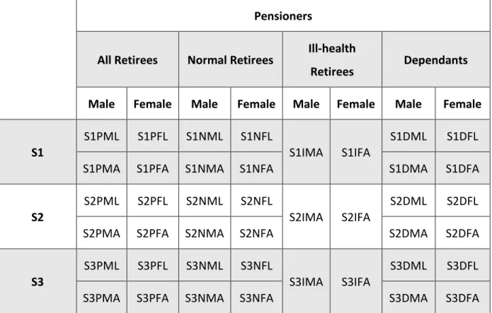
The Continuous Mortality Investigation, the main provider of mortality tables used at WTW, publishes regularly updated mortality tables for members based on experience conducted by Pension Schemes advisors and Insurance companies. The main tables used at Willis Towers Watson are the ‘S1’, ‘S2’ and ‘S3’ tables. These tables come from a set called “SAPS” which stands for Self-Administered Pension Schemes, which takes into consideration actual experience from the schemes.
21 The ‘S1’ series are base mortality tables based on 2000-2006 experience, collected by 30 June 2007; the ‘S2’ series are based on 2004-2011 experience, collected by 30 June 2012 and the ‘S3’ series are based on 2009-2016 experience, collected by 30 June 2017.
These series have base mortality tables specific for status and sex and can be presented in either lives or amounts (light or heavy). The tables start at age 16 and assume that by age 120 all members have already passed away. Because this report will only deal with pensioners, the tables to consider are:
Pensioners
All Retirees Normal Retirees Ill-health
Retirees Dependants
Male Female Male Female Male Female Male Female
S1
S1PML S1PFL S1NML S1NFL
S1IMA S1IFA
S1DML S1DFL
S1PMA S1PFA S1NMA S1NFA S1DMA S1DFA
S2
S2PML S2PFL S2NML S2NFL
S2IMA S2IFA
S2DML S2DFL
S2PMA S2PFA S2NMA S2NFA S2DMA S2DFA
S3
S3PML S3PFL S3NML S3NFL
S3IMA S3IFA
S3DML S3DFL
S3PMA S3PFA S3NMA S3NFA S3DMA S3DFA
Table 1 - Mortality tables published by the CMI. Source: IFoA 2019
For each of these, you can also have a suffix, either “_L” or “_H”, indicating if the table is light or heavy. The heavy tables are calculated using experience from members that don’t earn much income/pension and assume that people with lower income will live shorter. Light tables use the opposite membership and also assume exactly the opposite as what the heavy tables do.
22 If we consider the table S2PFA_L, we are looking into the experience of High income female members taken between 2004 and 2011 and with mortality rates weighted by amount (pension or salary).
4.2. CMI Mortality Improvements tables
Every year, the Continuous Mortality Investigation releases new life tables (IFoA 2019b) that take into account fresh information regarding mortality but also improvements that are expected to occur in the future, taking into consideration breakthroughs that have happened.
In order to start setting the model, it is important to understand how to calculate the mortality-improvement rate. This rate is defined by (Willets 1999) and is:
1 − 𝑞𝑥,𝑡 𝑞𝑥,𝑡−1, Where:
• 𝑞𝑥,𝑡 is the mortality rate for age 𝑥 at year 𝑡.
This takes into consideration the mortality rate that was verified for age 𝑥 during the year 𝑡 and compares it with the mortality for the same age group the previous year. This calculation gives back the percentage of mortality that was lost due to the improvement. Because we assume that mortality keeps improving, the rate is always smaller than 1 (and greater than zero). Throughout the years between 2011 and 2017, mortality improvements have been consistently lower each year, which is now revealing a trend in life expectancy (Palin 2017).
In practice, at the LSC, it’s used the improvements tables from the CMI. These are published every year and aggregate information regarding mortality for population of England and Wales, based on the data by the Office of National Statistics (ONS). The mortality projections are based on the CMI projection model above.
The tables are subdivided by the year they refer to, sex and adjustments to the mortality rates. The first year where mortality projections were calculated was 2009.
Tables are can also have adjustments to the rates (IFoA 2019b). This adjustments are multipliers in the range of 0% to 2% that reflect the extra improvement given to the
23 mortality rate to explain long-term mortality improvements: 0% means that the scheme does not consider any more long-term improvements than the one that is already reflected in the improvement table; 2% means that the long-term improvement is 2% higher each year.
24
5. Application of a Longevity Swap on a Real Client
During my internship at Willis Towers Watson, I had the opportunity to talk to some consultants about their experience with schemes that entered into a Longevity Swap. After a recommendation, I decided to use a scheme that did one longevity swap a few years ago. The purpose of this case study is to understand how the longevity swap impacts the scheme and to try and quantify the positive and negative impacts.
This scheme, that for confidentiality reasons will not be identified, is located in the UK, as it is the case with all the clients I worked on during the internship.
It is then important to understand how mortality has been in the past few years in the UK, to understand the background of the scheme’s membership.
The following graph aggregates the number of deaths per each year in England and Wales, per 100 thousand lives, between the years of 2001 and 2018 (ONS 2019)
Figure 1 - Deaths per 100.000 population in England and Wales between 2001 and 2018. Source: ONS 2019
As expected, longevity has been increasing for the regions of England and Wales in recent years, with the exception of 2015 where an increase in mortality happened, due to flu/respiratory reasons. 0 200 400 600 800 1000 1200 1400 1600 2001 2002 2003 2004 2005 2006 2007 2008 2009 2010 2011 2012 2013 2014 2015 2016 2017 2018
Deaths per 100.000 population
25 Taking this data into consideration, it makes perfect sense that Trustees appeal to Actuaries to consider de-risking mechanisms to protect themselves against longevity risk.
Such was the case for this scheme. Around 2012, the scheme decided to hedge the longevity risk and in 2013 the Trustees and the Company implemented a longevity swap.
At 2013, the scheme was covering liability for members of all statuses: Actives, Deferreds, Retirees and Dependants. Each status is divided into three sections, depending on the role that the employee had on the company. The longevity swap that was agreed upon, would cover the main section of the Retirees and Dependants population. From this point on, unless explicitly said otherwise, the reference to Retirees or Dependants is for the Main Section members.
The longevity swap covers liability for 5969 Retirees and 1518 Dependants. The financial assumptions used to calculate the liabilities were:
• Discount rate: 4.86%;
• Average Increases to pension in payment: 3.2%.
The demographic assumptions regarding mortality are dependent on the two types of members covered: members who have health benefits (like insurance) provided by the company and those who do not. The assumptions are different for both types because the company assumes that their insured members have better access to health treatments, which allows them to reduce their mortality experience, when compared with the non-insured members.
The scheme also assumes a lower mortality for females than the one they do for males. This is due to prudency. The CMI tables assume a lower mortality rate for females, but:
1. Most dependants are females;
2. Around 2/3 of the retired membership is male and assumed to be married to a female.
Therefore, the scheme believes that most of the future payments will end up being for females, who already have a higher longevity.
Table 2 shows the mortality assumptions agreed between the scheme and the insurance company. From this point on, all the cash flows from this scheme are going to be based on these assumptions.
26
Insured Non-Insured
Males Females Males Females
Base Table S1PMA_L S1PFA_L S1PMA S1PFA
Multiplier 100% 105% 105% 119%
Improvements 2013 CMI Mortality Projection Model with long term improvement of 1.50%
Table 2 – Mortality assumptions agreed between the scheme and the insurer. Source: Scheme’s Experience Information Form
5.1. Impact of changing the long-term longevity improvement rate
To understand the effects of the longevity swap, it is important to look at the scheme’s situation for these members had it not entered into the swap. For simplification purposes, it will be assumed that the scheme would use the same economic and demographic assumptions on a valuation with and without the longevity swap. This assumption may be realistic for the economic assumptions, as they are not affected by the scheme entering into the swap, but may not be very realistic regarding the mortality assumptions, since the insurer would always try to set very prudent assumptions. However, this scheme already uses very prudent assumptions for the calculation of their technical provisions, which means I do not expect the increase in prudency to be material for the results.
Using these assumptions, the total value of the liabilities for these members would be estimated as £1,810.6 million. Aggregated with the value of the rest of the membership that will not be covered by the swap, the total value of the liabilities would be £5,326.4 million. Taking this into consideration and also that the assets are £4,789.02 million, the funding level of the scheme would be 90%.
Because the cash flows for the members who will not be covered by the swap are not expected to change if the scheme decides to enter into a longevity swap contract, it is unnecessary to look into them. It is important, however, to compare the expected cash flows with the actual cash flows for the members that will be covered by the swap.
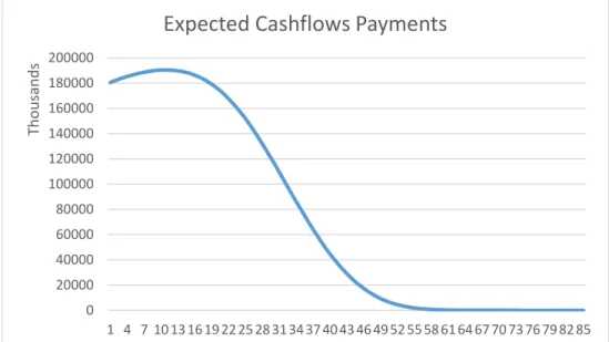
27 The following figure shows the expected cash flows if the scheme does not enter into a swap.
Figure 2 - Expected cash flows for the members that were covered by the longevity swap. Source: Author's calculations using Cash Flow Viewer+ 2019
From year 1 to 13, the cash flows are increasing every year, which on a first analysis was unexpected, but it is actually very easy to understand. The increases according to inflation create a negative impact for the scheme as they amplify the payments that are due, while the effect of mortality is actually positive for the scheme, as it reduces the amount of pension to be paid. What happens in these first thirteen years is that the effect of inflation is so much heavier than the effect of mortality that for the first years the scheme actually expects to pay more pension than in the year before. From year 13 on, the effect of mortality surpasses the effect of inflation and the expected pension in payment starts to decrease.
Another interesting point to notice on this graph is that by year 64 the pension in payment will be residual, suggesting that in 64 years almost all of the pension for these members has been paid out. Taking into consideration that the average age by pension of these membership is approximately 71 years old, this means that the scheme expects that by year 64 only the youngest members of the scheme. From this, is very clear how much prudency is set into these assumptions.
We are going to assume now that the long-term longevity improvements would be 0.25% higher per year. Taking this into consideration, the liabilities for the scheme would increase, because the members’ pensions would be, generally, in payment for longer than initially
0 20000 40000 60000 80000 100000 120000 140000 160000 180000 200000 1 4 7 10 13 16 19 22 25 28 31 34 37 40 43 46 49 52 55 58 61 64 67 70 73 76 79 82 85 Th o u san d s
28 considered. The liabilities would now be £5,374.9 million, meaning that the funding position decreased by 0.9%. In conclusion, the increase in the longevity assumption, decreased the scheme’s funding position from 90% to 89.1%.
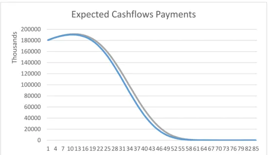
These are now the expected cash flows, assuming such a change:
From the graph above, it is very clear that the improvement in longevity resulted in higher cash flows. This was expected, because now we are assuming that members live longer, so they would be receiving pension for a longer period.
We have done the comparison of the scheme’s position with all the members, but now, looking into the liabilities for the members that would be covered by the swap. The initial expected liability was £1,810.6 million, while the expected liability if mortality decreases is £1,826.4 million. As we can see, for this population, the increase of 0.25% pa in the long-term longevity resulted in an increase of 0.8% of the liability for the main pensioner’s section. This impact would be around £16 million, which is not that immaterial, however, given that the percentage difference in liabilities is so small, only 0.8%, it becomes clear that the assumptions for mortality were already too prudent. If not, an increase in longevity would have had a higher impact on the overall liabilities.
0 20000 40000 60000 80000 100000 120000 140000 160000 180000 200000 1 4 7 10 13 16 19 22 25 28 31 34 37 40 43 46 49 52 55 58 61 64 67 70 73 76 79 82 85 Th o u san d s
Expected Cashflows Payments
Figure 3 - Comparison between the expected cash flows using 1.50% long-term improvement rate and the cash flows using 1.75% long-term improvement rate. Source: Author’s calculations using Cash Flow Viewer+ 2019
29
5.2. Impact of entering into the contract
The scheme decided to cover the liabilities of their pensioner’s main section. For reference, the liability that is not affected by the swap is of amount £3,515.9 million.
The implementation of the longevity swap will affect the expected payments that the scheme has to make, although the pension that the pensioners will receive will not change. The reason for this is the fact that the members’ actual pension is now paid by the insurer, while the scheme has to pay the expected pension plus the premium to the insurer. To make the transaction simpler, the scheme will pay the member’s actual pension and then:
1. If the actual pension is less than the expected pension plus the premium, the scheme would pay the pension to the member and the difference to the insurer; 2. If the actual pension is greater than the expected pension plus the premium, the
scheme would pay the whole member’s pension and be reimbursed of the difference between the actual pension and the expected pension plus premium by the insurer.
The main difference in entering into the longevity swap is that any change in the mortality rates would not affect the amount of the liabilities. Therefore, in the most simplistic set of mind, comparing with what was presented above and with the longevity hedge in force, the scheme would not expect to increase or decrease their funding level relative to these members. This is explained by the fact that the insurer is the one that is taking on the risk of the mortality rate changing.
5.2.1.
Case 1: Actual mortality lower than expected
In the case that mortality is lower than expected, the scheme will have more cash flows to pay than initially expected because members are living longer than anticipated. However, because the insurer agrees to pay the difference between the actual and the expected pension, the scheme’s liabilities would not change. The insurer would have to, therefore,
30 provision for the additional £15.8 billion in liabilities that resulted from the mortality being lower than estimated.
The liability that is not covered, is still sensible to the change in the mortality rate. This change would increase the non-covered liability to £3.5 billion and the funding level would be now at 89.3%.
Comparing the scenarios, if it so happened that there was a decrease in the mortality rates, the scheme’s funding level could drop from 90% to 89.1%, however, due to the swap, the funding level would actually just decrease to 89.3%.
5.2.2.
Case 2: Actual mortality higher than expected
On the other way round, suppose that mortality would have increased. In case the scheme entered the longevity swap, it would have to maintain the scheduled payments to the insurance company while the latter would be paying the actual pension to the members. Because mortality is assumed to increase, the pension in payment would be lower and the insurer would be making an immediate gain and would be reducing their liabilities, while the scheme’s liabilities would not change. However, had it not entered into the swap, the scheme would be making a gain and decreasing its liabilities.
Overall, the effect that the longevity swap would have on the scheme is that it would fix the liability amount in case there was any change in mortality rates. This feature is what makes longevity swaps so attractive in the first place. Whether members live longer than accounted for or not, the liabilities are not changing, so the scheme would not need additional contributions from the sponsor, due to longevity risk.
5.3. The effect of the premium
The insurer always demands a premium for accepting the risk that the scheme is trying to hedge. After all, longevity swap contracts are a type of insurance, in this case, against the possibility of unfavourable movements of the mortality rates.
31 In the case of this scheme, the premium demanded was 3.65% of all cash flows, payable yearly. This would mean that on top of the liability that the scheme would have to provision for, the £1,810.6 million, they would have to now provision for an extra £66.09 million, bringing the total liability of the scheme to £1,876.69 million.
The expected value of the liabilities in case there was a 0.25% pa increase in the long-term longevity improvements was £1,826.4 million. This means that the scheme would actually worsen its funding position by entering the swap. The funding position would now be 88.2%. Therefore, if this is the expectation that the scheme has for the longevity rates, entering into a longevity swap would not be worth it.
5.4. Actual Experience
In the sections above, we assumed an improvement of 0.25% pa of the long-term mortality rates and came to the conclusion that the improvement was not great enough to pay back the high premiums that are demanded. However, this increase in the mortality is a prediction that is being made. We were testing the longevity swap against a change of the assumption. In this section, we will be looking at the actual experience taken from the valuation of 2016.
Between 2013 and 2016, there were 365 male deaths, which correspond to £6.2 million of pensions that stopped being paid, while female deaths were 228, which correspond to an amount that stopped being paid of £1.9 million. This means that had the scheme not entered into a longevity swap, and considering that it assumes that 80% of the retirees are married, that their spouses receive 50% of the members’ pension in payment and that £1.1 million stopped being paid due to the actual dependants’ mortality, the scheme would have stopped paying £5.4 million in pension. Given that the scheme expected to stop paying £4.8 million in pension during the period, it would have actually made a profit of £0.6 million. This profit is explained by the member’s mortality being higher than expected, indicating, once again, that the mortality assumptions may be too prudent for this scheme.
32
5.4.1.
Payments from the scheme
Nevertheless, the scheme entered into the contract, meaning they are obliged to pay the expected cash flows to the insurer. Those were estimated, in thousands, three years ago as:
Year 1 Year 2 Year 3
119,161 119,697 120,135
Table 3 - Estimated cashflows for the three years between 2013 and 2016
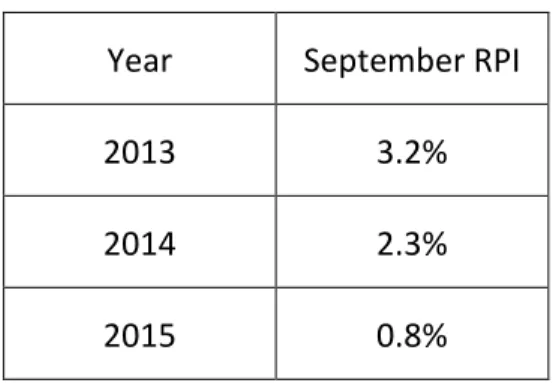
These, however, do not reflect the actual payments to the insurer, because these assume that there is a pension increase of 3.2% pa.
The actual increases in payments would be based on the September retail price index and they were, according to (WTW 2019):
Year September RPI
2013 3.2%
2014 2.3%
2015 0.8%
Table 4 - September RPI. Source: WTW 2019
In the first year, the inflation rate was exactly what was expected to be, so the actual payment to the insurer during year 1 was £119.2 million. For year two, though, the actual increase was much lower than expected so to get the actual cash flow that year, we remove the expected inflation (two increases of 3.2% that were given by the software) and then multiply by the actual increases, so 119,697,333.7
1.0322 × 1.032 × 1.023 =£118.7 million. As for
year three, the actual cash flow to the insurer is 120,134,500.8
1.0323 × 1.032 × 1.023 ×
1.008 =£116.3 million. Calculations above show the gain that the scheme had on the change in inflation rate, which was £1 million in the second year and £3.8 million in the third year.
33 Therefore, the cash flows from the pension scheme to the insurer are £119.2 million, £118.7 million and £116.3 million.
Focusing on the 2016 experience, the actual pension in payment to the members was £106.17 million , but the scheme has to pay £116.3 million to the insurer. Therefore, the members are paid their full pension, but the scheme still has to pay an extra £10.13 million to the insurer.
5.4.2.
Analysis of surpluses and losses
Three effects were considered in Chapter 3 as impactful when entering into a longevity swap. In this section, it will be understood how each of these affected the scheme.
5.4.2.1. Inflation rate effect
Above, it is explained in detail the effect that inflation had on each of the cash flows, due to the actual inflation being generally lower than the expected, which was 3.2%. This resulted in a gain of £4.9 million to the scheme.
5.4.2.2. Mortality rate effect
The mortality experience between 2013 and 2016 was irrelevant, because due to the longevity swap, the scheme paid what it was expecting to pay, so no gains nor losses from mortality experience. However, had it not entered into the swap, the scheme would have made a gain and reduced its liabilities because mortality was higher than initially expected. Moreover, had it not entered into the swap contract, the scheme would have saved the difference between the expected payment plus the premium and the actual pension. The premium paid that year was 3.65% of £106.2 billion, which is £3.9 million plus the difference between the expected and the actual payments, which is £10.1 million created a loss of £14 million for the scheme, just by entering into the swap.
5.4.2.3. Discount rate effect
The scheme assumed in 2013 that the discount rate would be around 4.86%, this rate is based on the gilt yields with allowances for expenses and future improvements. In 2016,
34 however, the actuaries and the trustees decided to introduce more prudency into their discount rate assumption, by decreasing the discount rate to 4%. This decrease meant that the scheme provisioned for less money than it actually needed to. In order to understand this, we discount the cash flows to 2013 using the original rate assumed and bring it to 2016 using the new rate. The implicit loss realized will be given by subtracting the actual value to be paid. This will give the impact that the interest rate had on this transaction. Therefore: 119,161,333.6 1.04 1.0486+ 118,653,461.6 1.042 1.04862+ 116,317,355.3 1.043 1.04863− (119,161,333.6 + 118,653,461.6 + 116,317,355.3) = −£5.8 𝑚𝑖𝑙𝑙𝑖𝑜𝑛.
Thus, entering into the longevity swap, created a loss for the scheme, as seen above, mainly because the actual mortality was larger than expected. As for the other effects, the scheme made a profit from the inflation rate experience, but a loss from the discount rate having changed, having an overall loss of £14.9 million.
The conclusion I must take from analysing this experience, is that the scheme hurt their funding level and could have actually improved if not for the longevity swap. But one thing must be taken into consideration: if it was clear that the scheme would make a loss in case the mortality rates did not decrease too much (from the beginning it was clear that a 0.25% improvement pa on the mortality rates would not be enough to compensate entering into the swap contract), why did it enter the swap anyway?
The answer is the obvious one: de-risking. In 64 years that the scheme is expecting to pay the pensions, mortality can actually reduce significantly due to, for example, medical breakthroughs or improvements in the lifestyle of members. The fact that the scheme has this contract in place will make sure that mortality rates will not influence the amount it will pay. Whatever the movement is on the mortality rates, the scheme’s funding is not expected to change drastically from mortality experience (though it would need to provision for the expected premium, which is 3.65% of the liabilities) and this means security for both the trustees and the sponsor. The scheme’s ultimate goal is to be able to
35 fund all the pensioners’ pension and not to make a profit and in this sense, entering into a longevity hedge is one of the ways to provision for higher longevity in the future.