i;~· ,.' __
:~~~~\
1'~1~;;'"
I <Li:Praia de Botalogo, nO 190/10° andar· Rio de Janeiro - 22253-900
Seminários de Pesquisa Econômica 11 (Japarte)
11
THE ROLE OF PROFITS IN
WAGE DETERMINATION:
EVIDENCE FROM US
MANUF AC1I'U'RING
11
MARCELLO ESTEV Ãü
MIT
Coordenação: Prof. Pedro Cavalcanti Ferreira Tel: 536-9353 'I ;."::
::)f '. \marf.
..
The Role of Profits in
Wage
Determination:
Evidence from US Manufacturing
Marcello Estevão
Stacey Tevlin*
Department of Economics - MIT
N ovember, 1994
*We benefited from insightful discussions with Joshua Angrist, Olivier Blanchard, Ricardo Caballero, Steve Pischke and Robert Solow. Beth Anne Wilson provided valuable suggestions. We would also like to thank the participants of the Money and Labor Lunch Seminars at MIT for their comments. We are responsible for all remaining errors. Financial support from CNPq-Brazil and the Federal Reserve Bank of Boston is gratefully acknowledged.
The Role of Profits in Wage Determination
Evidence from US Manufacturing
Abstract
We estimate the effect of firms' profitability on wage determination for the American economy. Two standard bargaining models are used to illustrate the problems caused by the endogeneity of profits-per-worker in a real wage equation. The profit-sharing parameter can be identified with instruments which shift demando Using information from the input-output table, we create demand-shift variables for 63 4-digit sectors of the US manufacturing sector. The LV. estimates show that profit-sharing is a relevant and widespread phenomenon. The elasticity of wages with respect to profits-per-worker is seven times as large as OLS estimates here and in previous papers. Sensitivity analysis of the profit-sharing parameter controlling for the extent of unionization and product market concentration reinforces our results.
1 Introduction
One of the main aims of theoretical work on wage formation is to understand why wages do not clear the market for labor. Many of the theories proposed to explain this phenomenon imply a positive correlation between profits and wages. While empirical evidence on inter-industry wage differentials suggests their structure may be related to profitability, direct tests of the effect of profits on wages in the US economy have found very small estimates. The lack of direct evidence casts doubt on the relevance of profits in wage determination. This paper provides strong new direct evidence that profit-sharing is an important part of wage determination not only in highly unionized sectors, but in the entire US manufacturing sector.
Previous studies of the US economy have failed to overcome the endogeneity of profits-per-worker in a real wage equation because they lacked appropriate instruments. In the next section, we show that basic bargaining models provide a justification for the assumption that
1
the profit-sharing parameter can be identified with instruments which shift demand for goods. We use information from the input-output table to create measures of demand for 63 4-digit sectors using the methods of Shea (1993a). The I.V. estimates show that profit sharing is a relevant and widespread phenomenon in the American economy.
The positive correlation between profits-per-worker and wages is predicted by several theo-ries. Efficiency-wage theories emphasize the unprofitability of wage cuts due to their effect on productivity. The falI in productivity may be due to costly worker monitoring (Shapiro and Stiglitz (1984)), or labor turnover costs (Salop (1979)). Akerlof and Yellen (1988) emphasize sociological and psychological reasons for wage stickiness based on the idea of fairness. In their model, firms pay higher wages to their workers when times are good. Thus, efficiency-wage arguments can explain real wage rigidity, wage differentials (since monitoring costs may differ across industries), and a positive relationship between firm profitability and the real wage.
Insider-outsider theories also predict a positive relationship between profits and wages. These mo deis explain insider power by their ability to be uncooperative with new employ-ees, causing adverse effects on overall productivity, and by the fact that the cost of substituting workers increases with the size of the workforce. The larger the rents of a firm, the larger the rent-extraction. See Lindbeck and Snower (1987) for a collection of papers in this tradition. The fundamentaIs of these mo deis give a rationale for the existence of unions that would be the institutional counterpart of insider power.
Some theories explain wage stickiness as insurance against bad times given by firms to
.. workers who are more risk-averse (the implicit contract models of Azariadis (1975) and Baily
(1974)). In these theories, the derivative of wage with respect to profit is positive and equal to the ratio between the relative risk aversion of firms and workers. As long as firms are not risk
2
neutra! (as assumed in the original papers), a positive rent-sharing parameter is predicted.1
The arguments described above generate a testable implication of the competitive approach
to the labor market. If the labor market were truly competitive, insider factors (like firm
profit~bility) would not be important for the determination of the real wage paid to a worker.2
The wage would be equal to the alternative wage. A series of studies using American, British and Canadian data, test the relevance of firm specific variables in an equation for real wage determination when controlling for alternative wage measures. In general, the null hypothesis of joint significance of firms' insider variables cannot be rejected. This conc1usion casts doubt
on the relevance of the competitive labor market approach.3
The problem with the above approach is that the results are not robust to alternative specifi-cations. Each paper inc1udes a set of insider variables but it is not c1ear what the interpretation for each coeflicient is. Our paper follows a different approach. We regress real wages on
profits-per-worker and the alternative wage.4 Previous studies that follow this approach find that
the profit-sharing coeflicient is positive and significantly different from zero.5 However, these
results find, in general, that the elasticity of real wages with respect to firms' profits is fairly small. Sanfey (1992), estimates an elasticity of wages with respect to profits-per-worker for
lSeeBlanchflower et ai (1992).
2Nickell and Wadwhani (1990) and Nickell and Kong (1988) call "insider variables" variables like finos' monopoly power, workers' bargaining power and technology. The unemployment rate, the average industrial wages and the unemployment insurance benefits would be examples of "outsider variables" .
3Dickens and Katz (1987) and Layard et ai (1991) describe these results in detail. Blanchflower et ai (1992) stress the fact that a model with mobUity costs can also generate a positive relationship between profits and wages. In this type of model, short-run wage leveIs couId respond to profit movements, but Iong-run wage ... leveIs would noto When they include Iags of the profitabUity measures in their wage equations, the sum of their
coefficients is still. positive and this alternative expIanation is rejected.
4Some ofthe variabIes we choose not to include separateIy (e.g. technoIogy, demand, and market power) are l i ' .'. ... . .
sumDlariz~Q. by profits-per-worker, others (e.g. unionization) are part of the rent-sharing parameter.
l>SeeAbowd and Lemieux (1993), BIanchflower et ai (1992), Caruth and Oswald (1990), Christofides and Oswald.(1992), Currie and McConnell (1992), Denny and Machin (1991), Hildreth and Oswald (1993) and Nickell and Wadhani (1990).
the American economy of .05, while Blanchfiower et ai (1992), estimate elasticities between .02
and .04. Therefore, although the profit-sharing parameter is significantly different from zero, its size suggests that the competi tive labor market paradigm may not be far from the truth. Studies that use data for other countries tend to find similar results. This approach yields a robust result and offers a useful benchmark.
The general problem with these results is that they do not have good instruments to identify the profit-sharing parameter. The simultaneity between wages and profits-per-worker generates inconsistent estimates of the wage elasticity with respect to profits. Abowd and Lemieux (1993) estimate a higher elasticity for Canada (0.195) using import and export prices as instrumental variabIes. They argue that externaI prices are good instruments because they represent exoge-nous shocks to product market conditions due to the fact that Canada is a small open economy.
AIthough their work yields evidence against the competitive paradigm for the unionized fraction
of the Canadian labor market there are two reasons to believe that the US labor market is a more interesting case. First, there is a popular belief that the US labor market is very elose to the competitive labor market paradigm. Second, their results are less surprising because they use data from union contracts while the data we use represents the entire US manufacturing sector.
The main difference between our study and previous studies is the empiricaI strategy foI-lowed here. As the next section will show, demand shocks can be used to identify the
profit-- sharing parameter under plausible assumptions. We solve the simultaneity problem between
~ wages and profits-per-worker using information from the input-output table to select good
demand-shifters for some 4-digit sectors of American manufacturing. The methodology is briefiy
4
described in the body of the paper.6 The sample used is representative of the whole US
man-ufacturing sector.7 Our OLS estimates generate an elasticity of 0.05 which matches previous
results for the American manufacturing sector. However, using the LV. procedure, we estimate the elasticity of real wages with respect to profits-per-worker at around 0.33. The magnitude of our estimates shows that profit sharing is an economically relevant phenomenon in the USo Our approach also permits us to control for the extent of unionization and the degree of monopoly power in the goods market, shedding light on the relationship between insider variables and the degree of profit-sharing.
The paper has four other sections. The models presented in the next section provide a framework for the empirical section and, in particular, organize the discussion on simultaneity and measurement error issues. Section 3 describes the empirical methodology to be used, including the choice of instruments and the specification of each variable used in the estimation. Section 4 reports results for different specifications of the basic equation relating real wages and profits-per-worker derived in section 2 and provides our basic estimate for the profit-sharing coefficient. In addition, we analyze how insider variables affect this elasticity, real wages and profits-per-worker. The last section concludes.
2
Wages and profits
Including profitability measures in a real wage equation yields inconsistent estimates when OLS is used. Let us write the basic equation to be estimated as:
..
6For more details, we direct the reader to Shea (1993a).
7See Appendix 2 for comparisons between our sample and the entire manufacturing sector.
5
J
e,"e __ "~ _ _ _ _ _ _ _ _ _ _ _ _ _ _ _ _ " " " " " ' ' ' ' ' ' ' ' - ' ' ' ' ' ' ' ' ' _ _ _rr
W = "(-+Z+1]
N (1)
where "( is the profit-sharing parameter; W is the real wage; ~ is profits-per-worker; Z is a
. measure of the alternative wage; and 1] represents relevant omitted variables.
The estimation of equation (1) is prohlematic for several reasons:
• First, wages enter directly in the formula of the profits-per-worker variable with a negative signo Everything else constant, there is a downward bias in estimates of "(. Profits-per-worker can be written as:
(2)
where Af(N) is value added; and A is the revenue-shifting parameter.8
The following regression shows the OL8 results for a panel of 450 4-digit U8 manufacturing industries. Year dummies are inc1uded to capture the effects of the alternative wage and any other year effects.
(OLS) W .040 ~
+
Yeardummies R2=
0.26(.002)
The problem of the downward biased "( can be solved if we estimate equation (2) using the real value added-per.worker as an instrumental variable. Assuming that the only .source of simultaneity between wages and profits comes from the inclusion of wages in
8Ingeneral, the parameter A will be a function of the technology and the demand for the final good. For a simpl~ example, assume that labor is the only input, the production function is Cobb-Douglas, X = A' NQ , X =
qutput, A'
=
teclmological shocks, and that the product demand curve is, X=
Ali p-k, Ali=
demand-shifter,k
=
elasticity of demando In this case, A=
A' * AI/f.the profit-per-worker formula, this LV. strategy would yield consistent estimates of f.9
(IV) W - .082
(.002)
~
+
YeardummiesThe LV. estimate of the profit-sharing parameter is larger than the OLS estimate, as
ex-pected. Unfortunately, there are other possible sources of simultaneity between wages and
profit-per-worker. In these cases, real value added-per-worker is not a good instrumental
variable and we need to look for an alternative instrumento
• Most of the papers in this literature measure profits as the difference between sectoral (or firm) value added and the wage bill. The failure to take into account the cost of capital generates measurement error problems in real value added-per-worker. Several authors
(Blanchfiower et ai (1993), for instance) take out depreciation allowances and the rental
cost of capital, but the implicit hypotheses built in the calculation of these variables are
sources of measurement errors in and of themselves. In this case, 1] in (1) represents
measurement error and OLS estimates of f will be inconsistent.
• Even if both of the above problems were not present, wages and profits-per-worker are endogenously determined if firms change employment to adjust for autonomous variations in wages. As we are going to illustrate in the next section, this is the case in most bargaining models.
• Finally, as pointed out by Abowd and Lemieux (1993), heterogeneity among sectors may
cause inconsistent estimates of f if fi, the profit-sharing parameter of sector i, is correlated
9The variables are in natural logarithms. The regressions are run in first-differences to correct for sectoral fixed effects. The standard error (in parentheses) ofthe estimated parameter is calculated assuming the residual term follows a MA(l). For more information about the data see subsection 3.2.
Oi
with
*.
.
8ince several papers, including this one, are interested in the average profit--sharing parameter for the whole economy, we rewrite (1) as:
(3)
17:
represents other stochastic terms not inc1uded in (1).In this case, if "fi is correlated with profits-per-worker (sectors with higher
profit-per-person share less profit with their workers, for instance), the residual term will be corre-lated with the regressor and the OL8 estimator will be inconsistent.
Let us turn to some simple bargaining models. These models will provide some structure
for the analysis of the results and highlight a way to identify the parameter "f in equation (1).
2.1 Efficient bargaining
The first model to be presented assumes that workers and firms bargain over wages and
em-ployment in order to maximize the joint surplus of their economic activity.lO If both parties do
not reach an agreement they receive fallback incomes. Workers maximize the surplus expected utility derived from their income (expected utility minus a threat point defined by the fallback wage). The firm maximizes its surplus profits. We assume that the fallback or "strike" profit is equal to zero. The source of workers' bargaining power comes from their ability to act as a group. The ability to act as a group generates bargaining power, which is represented by the
lOThis explains the name "efficient bargaining". There is a discussion on what is the most appropriate specification for the objectives of the bargaining processo Layard et al (1991), chapter 2, shows the arguments against the efficient bargaining setup and in favor of the "right-to-manage" model where firms and workers bargain over wages only (to be presented below). Blanchflower et al (1992), for instance, use the efficient specification because the "right-to-manage" would be based upon "an explained inefficiency" .
parameter, J.L.
The N ash bargaining process can be summarized by maximization of:
(4)
where <I> is the surplus expected utility of a representative worker and
rr
is the profit leveI ofthe firmo The surplus expected utility of a representative worker can be defined as:
<I> = N(v(W) - v(Z)) (5)
where W is the real wage; N is the employment leveI; Z is the alternative wage; and v(x)
measures the utility derived by an individual from income x.
Equation (5) assumes that the alternative wage received by a worker if fired is also the fallback wage in case of a di5agreement. Additionally, we choose the units of N 50 that N can
also be interpreted as the probability of employment. The expected alternative income, Z, is
a function of "outsider" variables: the unemployment rate, unemployment benefits, and the economy-wide average wage rate.
Let us write profits as:
rr
= Af(N) - WNwhere A is a revenue-shifting parameter.
The first-order conditions we get from maximizing (4) with respect to W and N are:
9
(3 II = v(W) - v(Z)
N v'(W) (6)
W =
(3~
+
Af'(N) (7)Linearizing v(Z) around W, throwing away higher order terms, and rewriting both (6) and
(7), we get:
(8)
AJ'(N)
=
Z (9)(3
=
r:;
is the relative bargaining power of workers.In this model, firms hire workers untillabor productivity is equal to the alternative wage a worker would receive if fired. Therefore, the hiring decision of firms does not depend on the contracted wage. This is the "strongly eificient" bargaining case. Variations in the utility function of workers may generate the case where firms hire workers on the labor demand curve
ar where they equate labor productivity and a weighted average of Z and W. For instance, if
we write the worker's utility as,
NlAl (W - Z)1A2
10
8IBUOTEC~
MARIOH~NR'(lUE
SIMONSEIthe optimal contract curve is:
AI' = (1 - J.Ll) W
+
J.Ll Z J.L2 J.L2..
The wage equation is still (8), where (3 is the ratio between J.L2 and the exponent on
profits-per-worker in the Nash bargaining function. If J.Ll = O, we have a situation where workers do not
care about employment. Incumbent workers may not care about employment if layoffs follow a seniority rule and the positions of incumbent employees are protected by substantial labor
turnover costs.l l
In either case, the profit-sharing coefficient, (3, is independent of changes in
profits-per-worker within each sector and changes in the revenue-shifter parameter, A, affect wages only
through variations in the profits-per-worker variable. Therefore, variations in market conditions,
which are summarized by shifts in A are transmitted to wages only through variations in
profits-per-worker. By identifying exogenous changes in A, we are able to provide consistent estimates
of the profit-sharing parameter using these revenue shifts as instruments.
2.2 Right-to-manage models
Some authors argue that bargaining between firms and workers is not efficient. Layard et al
(1991) present factual evidence that both parties do not bargain over employment after all.
Even if workers care about employment they may bargain over wages with the firm and let it
..
fix the employment leveI that maximizes profit. The Nash bargaining function to be maximizedis:
llSee Lindbeck and Snower (1990) for an example of such a model.
i
11 I
"
n
= (N(W)(v(W) - V(Z)))1LI11-1L(10)
Differentiating (10) with respect to W, using the fact that firms maximize profit, and
linearizing v(Z) around W, we get:
11
W=,-+Z
N Af'(N)=
W (11) (12)The innovation introduced by this mo dei is that the profit-sharing parameter will not be
equal to
/3,
the relative bargaining power of workers, but will be a function of/3,
profits-per-worker and the elasticity of labor demand, , =
,(/3,
~, f).Now, ~ cannot be considered a suflicient statistic for the product market conditions.
Changes in A may affect real wages through changes in the elasticity of labor demando
Assum-ing that € is constant allows the identification of (11) with revenue shifters.
The parameter of interest in equation (11) depends on the profits-per-worker variable. This dependence exacerbates the simultaneity problems caused by heterogeneity in , which were pointed out earlier. In order to solve this problem without assuming any specific function for " we linearly approximate , with respect to profits-per-worker:
(13)
where ~ is average profit-per-worker.
..
We assume that the residual ofthis approximation is insignificant. Notice that the coefficient
rI
is interesting in and of itself. Looking at the time dimension, a negativerI
means thatprofit-sharing decreases in good times and increases in bad times. Considering the cross-sectional dimension, sectors that have consistently higher profitability than the sample average, share
a smaller percentage of profits-per-worker. The opposite is true if
rI
>
O. We give furtherinterpretations for this coefficient in the results section. The equation to be estimated in this case is:
(14)
T]i is a stochastic term representing exc1uded variables and other random shocks.12 Equation
(14) can be consistently estimated if the instrumental variable used to identify revenue shifts
is not correlated to the terms inc1uded in T]i.13
To summarize the last two subsections: revenue-shifters identify the profit-sharing
param-eter in common bargaining models. If we assume the right-to-manage model is the best
de-i:aUsing the specmcation in this simplified model, we can write "Y(.) as
8N 1
i= 8W N <O
i is the semi.:..elasticity oí labor demando We can identify (14) under the hypothesis that this semi-elasticity is constant. The equation is also identmed if the elasticity oí labor demand is constant, f
=
iW=
c. In this case, we can specify an approximate linear specmcation íor the relationship between real wages and profits-per-worker, if we first linearize "Y with respect to wages, rewrite equation (11), and then linearize both the coefficients oí ~ and Z. The final equation in this case would be:fii fii (fii 0) (fii 0) I
W="YO-+eOZi+"Yl- - - - +e1Zi - - - +1];
Ni Ni Ni N Ni N
1]~ is.a stochastic term representing exc1uded variables and other random shocks.
The interactive term between measures oí the altemative wage and profits-per-worker proved to be insignifi-cant in our regressions and it was exc1uded from the specmcations .we present in the results section.
13We use the square oí the revenue-shifters as an extra instrumento
•
scription of the way firms and workers bargain over key labor market variables, additional assumptions on the elasticity of demand for labor are required in order to guarantee
identifica-tion. If we assume bargaining is efficient, no such assumptions are necessary .
3
Empirical methodology and data description
3.1 Demand-shifters
The last section made the case for the use of revenue-shifters as good instruments for estimation of linear profit-sharing relationships. Either neutral technology shocks or exogenous variations in the demand for goods may be used as revenue shifters. We choose exogenous changes in demand as our revenue shifters because we can build this variable with a high degree of
certainty that it is a good proxy for exogenous movements in A.
We perform a panel data analysis for the 4-digit sectors of the American manufacturing sector. One way of getting good demand shifters for this database is to use the input-output approach described in Shea (1993). Shea uses information from the input-output tables for two-, three-two-, and four-digit industries to choose variables that should be correlated with demand
shifts of a particular 4-digit sector. Output of sector j is a good demand-shifter for sector i
if sector j demands a large share of sector i's output, but sector i, and other sectors closely
related to it, comprise a small share of the production costs to sector j. The first condition is
to insure that output of sector j is relevant for identifying demand shifts. The second condition
,., is to minimize the possible sensitivity of the output of sector j to price variations in sector i.
Let us call the demand share of sector j, DS, and the cost share of sector i,
es.
Shea (1993a) shows that the asymptotic bias in the IV estimates of the supply elasticity 14
obtained when using the input-output approach to select instruments is decreasing in the ratio, DS/CS. For a given ratio, increases in DS should increase the correlation between final and intermediate output. Using Monte-Carlo simulations, Shea shows that this increased correlation improves the small sample behavior of his estimates over some range. Therefore, variables with high DS/CS ratios are good demand-shifters, in the sense that they identify a supply elasticity
with small asymptot~c bias. Since we need good demand-shifters, the same results apply to our
approach.14
This general rule is not enough to select potential instruments for sector i. It is important
to impose rules on the process of instrument selection that minimize the influence of common supply shocks between both the sector we use as an instrument and the sector for which we need
an instrumento For instance, sectors with the same two-digit SIC code as industry i are not
eligible instruments for industry i. This prohibition reflects the assumption that supply shocks
are highly correlated within a two-digit industry. For the same reason, industries belonging to different SIC groups that are subject to similar supply shocks were not used as instruments
for one another.15 In addition, the cost share data used in the instrument selection is the cost
share of the two-digit sector containing industry i. For more details, see Shea (1991).
In summary, instruments chosen by this approach are good proxies for exogenous variation
in A, the revenue-shifter. In other words, it is not plausible that variations in the price of
sector i have a significant impact on the output of sector j because the share of sector i in
sector j's cost is smaI!. This methodology tends to generate instruments at a higher leveI of
.. aggregation than the sector for which we are instrumenting. Furthermore, many of the variables
14The threshold values we used are DS/CS > 3 and DS > 0.15, the same used by Shea.
15This is the case for apparel and textile industries (SIC 23 and 22), primary and fabricated metais industries (SIC 33 and 34), machinery and eletricai machinery industries (SIC 35 and 36).
we use are ideal demand shifters when significantly related to sectoral output because they are obviously exogenous. Government defense spending is a good example of this. Changes in defense spending are more related to political and social movements than to specific 4-digit industry supply shocks.
The list of potential instruments for 150 4-digit industries that follow these rules can be found in Shea (1992). The problem with this list is that it does not guarantee that the
rela-tionship between the instrumental variable candidate and the output of sector i is a result of
their input-output link. If the candidate follows business cycle variations closely, it may be a
poor instrumento In this case, it is plausible to assume that the instrument does not
repre-sent exogenous shocks to revenue in sector i, because the cost variables in this sector may be
significantly correlated to the business cycle themselves.
In order to solve this problem we pretested the potential instruments for relevance once busi-ness cycle variations were purged from the data. First, we regressed the potential instruments
on business cycle measures and got the residuaIs from this equation.16 Then we regressed
out-put growth on the residual instrument growth to check for instrument relevance. We discarded
instruments which had low T
*
R2 statistics or were negatively correlated to the regressor.l7The sectors chosen after this checking process are reported in Appendix 1.
Some sectors have only one good instrument, while others have more than one. In order to select one vector of instruments among all the available possibilities, we maximize the criterion which is used to guarantee instrument exogeneity. Hence, we choose the instrument which has the.highest ratio of OS to CS. Using other criteria to generate the demand-shift vector generates
16Different measures were used. The final regressions use the total manufacturing price and production as business cycle indicators. The results are insensitive to the choice of other indicators.
17Although only a few instruments produce a negative correlation to output, we discarded them since sys-tematic demand shocks should be related to variations in output in the same direction.
•
similar results to those reported in the next section.
3.2 Data
Most of the data in this paper comes from the Productivity Database compiled by Wayne B. Gray. For more details see Gray (1992). The basic original source is the Annual Survey of Manufactures. The wage is computed as the ratio of payroll to employment divided by the Consumer Price Index. The data on payroll and employment include production as well as
non-production workers. Profits are computed as Value of Industry Shipments
+
Inventory change- Payroll - Costs of Materials.18 Profits were then divided by employment. We proxied for the
alternative annual average wage for each sector by including the average annual manufacturing wage (deftated by the CPI) and the unemployment rate for the whole economy in the estimated equation. Though data on production worker hours are available, we use the total number of workers as the employment variable because we want a sample which is representative of the
whole labor force. 19
For those industries whose instruments were other 4-digit industries, we used output created
from the Gray database.20 For those sectors whose instruments were two-digit industries, output
was taken from Citibase. The sources of the additional instruments are available from us upon request.
18The last term is deftated by the Price of Materials Deftator while the other terms are deftated using the Value of Shipments Deftator.
19Using wages per production worker-hour and profits per production worker-hour yields similar results to our estimates. Using average work hours of production workers as a proxy for average work hours of the total workforce also does not change the results. See the next section for further details.
20
y
=
ValueofShipmentst+
Inventoriest - Inventoriest_l Valueof ShipmentsDeflatort17
4
Results
We discuss the basic results first, then turn to how these results change when we adopt alter-native specifications, control for the degree of firms' monopoly power in the goods market, and control for the extent of unionization. The equation we estimate is:
(16)
ai represents industry specific effects; TJit is a stochastic term representing excluded variables
and other random shocks.
We assume that the alternative wage of a worker is the same for everyone, Zit = Zt. All
variables enter as naturallogarithms. We take first-differences to wash out fixed industry effects.
The final specification is:
(17)
Under the assumption that TJit is white· noise, we calculated the standard errors of our
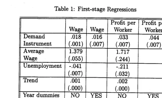
estimated parameters assuming that tlTJit follows an MA(1) processo Table 1 shows the first
stage regressions for real wage and profits-per-worker. It should be noted that it is not clear a
priori what the relationship is between changes in demand and changes in profits-per-worker and
wages. The effect of increases in output on profits-per-worker will depend on labor productivity, for instance. The results show that increases in demand increase profits-per-worker and wages.
All the other exogenous variables are relevant as well. We also include a specification with time
dummies to capture time effects. This specification is superior to the one that includes just
the alternative wage, unemployment and a trend, because it takes care of these variables in addition to other relevant omitted variables without cross-sectional variation.
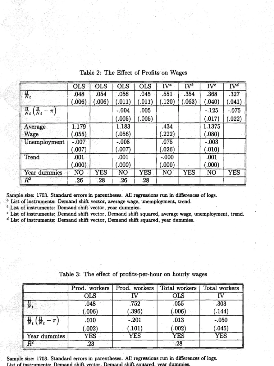
Table 2 presents the OL8 and the IV results. The OL8 estimates of the profit-sharing
coefficient vary from .045 to .056, which are of the same order of magnitude as previous results.
The specifications induding the unemployment rate and the average industrial wage produce the expected signs, although the coefficient for unemployment is statistically insignificant. The coefficient of average industrial wages is dose to one as expected. The quadratic term is not significant in the OL8 estimates.
The IV results show a different picture. The profit-sharing coefficient in the preferred specifications of columns 7 and 8 is six times larger than the OL8 estimates. Estimates in column 5 show the importance of including time dummies and the quadratic term in (17). This is the only specification that generates a positive sign for the coefficient on unemployment, a
small value for the coefficient of the average industrial wage and a .55 profit-sharing parameter.
The preferred specification is in column 8 where time dummies and the quadratic term are included. We estimate a profit-sharing parameter for the American manufacturing sector equal to .327.
We find a consistently negative coefficient for the quadratic termo This result shows that firms share a smaller (larger) proportion of their profit when profits-per-worker increase (de-crease). This fact is consistent with a simple right-to-manage mo dei where the profit-sharing parameter is inversely related to firms' profitability. Profit-sharing diminishes in good times
~ and increases in bad times. Firms that are less profitable than average share more than more
profitable firms. We give further evidence on this point below.
One could argue that the fact that we use variables that are not corrected by the number
of hours each employee works may be biasing our IV estimates upward. In this scenario, the detected wage variations when the conditions in the product market change could be merely capturing the fact that average hours of work are positively related to demand shocks. Table 3 gives the results using two different definitions for the hourly wage and the profit-per-hour variables. The first two columns use the data for production workers. The last two columns use the average hours of production workers as a proxy for the average hours of all workers in a sector. Both OLS estimates are very similar to the results listed in the fourth column of Table 2. The IV results show that the point estimate for the profit-sharing parameter using production worker data is larger than the profit-sharing parameter when data for the whole labor force are used, although this difference is not statistically significant. The results for the total labor force in column four are equivalent to the results in Table 2.
Blanchfiower et ai (1993) test two alternative hypotheses for the positive coefficient on
profits-per-worker. First, if the production function is Cobb-Douglas, we may be capturing an inverted labor demand curve. Wages will be positively related to profits-per-worker, even if workers and firms do not bargain over wages, because they are negatively correlated to employ-ment and variations in employemploy-ment cause smaller variations in profits in the same direction.
So, if employment increases because wages decrease (workers' preference changes, for instance),
profits are going to increase less than proportionately and profits-per-worker are going to be positively related to wages. The methodology we follow here dispenses with this hypothesis
automatically because in the Cobb-Douglas case ~ is independent of shifts in demand (see
McDonald and Solow (1981)). Therefore, we should not be able to identify equation (17) using demand-shifters as instruments - which is clearly not the case.
Second, the competitive model with labor mobility costs may also generate a positive
rela-20
8IBlIOTEC~ MARIO HENnlQUE SIMONSEN
•
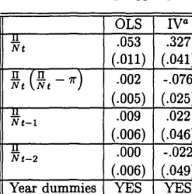
tionship between profits-per-worker and wages in the short-run.21 We introduce lags of ~ in
our regressions in order to pick up this dynamic effect. Table 4 shows that the inclusion of these lags does not alter our results. The sum of their coefficients is essentially the same as if the Iags were omitted. Additional specifications where lags of the interactive term and higher order lags were induded generate the same resulto Because the competitive model with labor mobility costs predicts a long-run elasticity of zero, we can reject it in favor of a bargaining modeI.
The profit-sharing parameter may vary across sectors for several reasons. The next set of
results focuses on two different sources of variability in 1'0. First, some sectors produce more
economic rents than others and there is no reason to assume that they share the same proportion of their profits. In other words, we are saying that the profit-sharing parameter, evaluated at
average profits-per-worker, 1'0, can be different for groups of firms with different ~.
One way of testing this effect is to break our sample using an exogenous variable which represents the ability of a sector to produce rents. We split our sample using a 4-firm concen-tration index for each sector. This index is a proxy for firms' market power and their ability to generate economic rents. Table 5 breaks the sample in two: sectors that have market power below the median levei and sectors that have market power above the median leveI. The IV results show that profit-sharing is inversely related to market power, although the difference is not statistically significant due to high standard errors in the low market power sample. In other words, the higher the degree of monopoly power in a sector, the higher the
profits-per-worker and the real wage paid, but the lower the proportion of profits that are shared.22 This
21 This result is driven by the fact that in the short-run the labor supply curve would not be Bat, as in the traditional competitive model, but positively sloped.
22The matrix of correlations of wage, profits-per-worker, the market concentration index and the extent of
21
•
result is not very sensitive to how we split the sample.
Note that this effect is similar to the one suggested by the negative sign of the quadratic term coefficient. The difference in monopoly power across sectors cause differences in profitability which contributes to wage variation across industries, but the effect is dampened by the behavior of the profit-sharing parameter. Thus, the relationship between the profit-sharing parameter and market power diminishes the cross-sectional variability of wages. This result is robust to different breakpoints.
Another source of heterogeneity in 'Y is the variability of workers' bargaining power between
sectors. We use the extent of unionization variable available in the NBER trade database, and described in Abowd (1990), to break our sample in two groups: sectors that have a high leveI of union penetration and sectors that have a Iow leveI of union penetration. Table 6 shows the OLS and IV results for both subsamples. Sectors where workers have little bargaining power (proxied by the extent-of-unionization variable) yield a higher profit-sharing parameter than sectors where workers have strong bargaining power, a puzzling resulto
Though this difference is statistically significant, different breaks in the sample generate
unionization is: W n. Cooc. Unioo. W 1.000 II .410 1.000 Nt Cooc. .468 .254 1.000 Unioo. .517 .113 .211 1.000
Regressions of wage and profits-per-worker on market concentration and extent of unionization captures the effect of one of these variables controIling for the other. Standard errors are in parentheses .
w =
.10 *cooc+
. 35 *unioo (.006) (.014) II=
.12 *cooc+
.27 *unioo Nt (.017) (.042) 22j
different results. Table 7 splits the sample in three: low, medium and high unionized sec-tors. The results point to a u-shaped relationship between the extent of unionization and the profit-sharing parameter, although the differences between the coefficients are not statistically sigiiificant. Therefore, the empírical evidence is dubious with respect to the effect of union-ization on the profit-sharing parameter. It seems that the previous results were driven by the behavior of sectors around the median value for the extent of unionization. However, since bargáining power may come from a variety of sources in our sample and not just fram the extent of unionization, the results are less surprising. Further research using different proxy variables for workers' bargaining power is necessary in order to clarify this point.
5
Conclusions
Ourwork sheds new light on tests of labor market competitiveness. Previous authors claim that the very small elasticities of wage with respect to profits-per-worker they find are relevant nonetheless because profits-per-worker are so variable across industries that even a small elas-ticity generates an impact on wages. We estimate an elaselas-ticity which is six times as large as the previous results and our own OL8 estimates (.33 as compared to .05). Changes in profits-per-worker have a relevant impact on wages regardless of the variation in profits-per-profits-per-worker. Our methodology also provides evidence against alternative explanations for the positive correlation between profits-per-worker and wages such as a neoclassical model with labor mobility costs and a simple profit-maximization model with Cobb-Douglas technology.
Additionally, we study the sensitivity of the profit-sharing parameter to variations in its determinant.s. Changes in profits-per-worker have a dampening effect on profit-sharing. This
effect is consistent with a simple right-to-manage model where the profit-sharing parameter varies inversely with profits-per-worker. More evidence on this point was obtained by splitting the sample using measures of industry market power in the goods market. Sectors that have more monopoly power tend to have more rents-per-employee and pay higher wages, but they share a smaller proportion of profits.
When we used the extent of worker unionization in a sector as a proxy for worker bargaining power we got puzzling results. The relationship between this variable and the profit-sharing parameter is not robust to different sample splits. This fact seems to be driven by the outlier behavior of sectors around median values of unionization. Our final evidence on this question establishes a weak u-shaped relationship between the extent of unionization and rent-sharing behavior. Further research is needed to understand the effect of workers' bargaining power _ including bargaining power due to forces other than unions - on profit-sharing.
Table 1: First-stage Regressions
Profit per Profit per
Wage Wage Worker Worker
Demand .018 .016 .033 .044
..
Instrument (.001) (.007) (.007) (.007) Average 1.379 1.717 Wage (.055) (.244) Unemployment -.041 -.211 (.007) (.032) Trend .001 .002 (.000) (.000)Year dummies
NO
YESNO
YESR~ .28 .28
.05 .10
Sample size: 1703. Standard errors in parentheses. All regressions run in differences of logs.
..
li
Table 2: The Effect of Profits on Wages
OL8 OL8 OL8 OL8
Iya
Iyb
IYc
!!. .048 .054 .056 .045 .551 .354 .368 Nt (.006) (.006) (.011) (.011) (.120) (.063) (.040)
~t (~t
-7r)
-.004 .005 -.125 (.005) (.005) (.017) Average 1.179 1.183 .434 1.1375 Wage (.055) (.056) (.222) (.080) Unemployment -.007 -.008 .075 -.003 (.007) (.007) (.026) (.010) Trend .001 .001 -.000 .001 (.000) (.000) (.000) (.000)Year dummies NO YE8 NO YE8 NO YE8 NO
R"I. .26 .28 .26 .28
Sample size: 1703. Standard errors in parentheses. All regressions run in differences of logs.
a List of instruments: Oemand shift vector, average wage, unemployment, trend.
b List of instruments: Oemand shift vector, year dummies.
Iya
.327 (.041) -.075 (.022) YE8c List of instruments: Oemand shift vector, Oemand shift squared, average wage, unemployment, trend.
d List of instruments: Oemand shift vector, Oemand shift squared, year dummies.
Table 3: The effect of profits-per-hour on hourly wages
Prod. workers Prod. workers Total workers Total workers
OL8
IY
OL8IY
.!!. .048 .752 .055 .303 Nt (.006) (.396) (.006) (.144)~t (~t
- 7r)
.010 -.201 .013 -.050 (.002) (.101) (.002) (.045)Year dummies YE8 YE8 YE8 YE8
11.2
.23 .28Sample size: 1703. Standard errors in parentheses. All regressions run in differences of logs. List of instruments: Oemand shift vector, Oemand shift squared, year dummies.
•
Table 4: Estimations including lagged profits-per-worker
OL8 Iva .!!. .053 .327 Nt (.011) (.041)
~t (~t
-7r)
.002 -.076 (.005) (.025) 1!. .009 .022 Nt-l (.006) (.046) !! .000 -.022 Nt-2 (.006) (.049)Year dummies YE8 YE8
R'l. .29
Sample size: 1642. Standard errors in parentheses. All regressions run in differences of logs.
List of instruments: Contemporaneous and two lags of the demand shift vector, demand shift squared, year dummies.
Table 5: Produet Market Concentration
OL8 OL8 IV IV
Low Cone High Cone Low Cone High Cone
!!. .100 .025 .789 .300
Nt
(.025) (.011) ( .260) (.056)
~t (~t
-
7r)
-.008 .002 -.348 -.052(.011) (.006) (.150) (.024)
Year dummies YES YES YES YES
ff.2 .31 .31
Obs. 821 868 821 868
Standard errors in parentheses. All regressions run in differences of logs.
List of instruments: Demand shift vector, demand shift squared, year dummies. The product market concen-tration index is the 4-firm concenconcen-tration index found in the NBER database. The sample was broken at the medium value for market concentration, 41.0%. The results are robust to different breaks.
27
•
i
Table 6: Extent of unionization
OL8 OL8
IV
IV
Low Union High Union Low Union High Union
!!. .066 .018 .620 .270
Nt
( .015) (.174) (.083) (.054)
~t (~t
-7r)
-.009 .023 -.140 -.069(.007) (.008) (.420) (.039)
Year dummies YE8 YE8 YE8 YE8
R
2 .28 .28Obs. 827 893 827 893
Standard errors in parentheses. AlI regressions run in differences of logs.
List of instruments: Demand shift vector, demand shift squared, year dummies. The extent of unionization variable is the one constructed by Abowd and Farber (1990). The medium value for the extent of unionization for production workers is 48.5%. This result is not robust to different break points. See Table 7.
Table 7: Extent of unionization
IV
IV
IV
Low Union. Medium Union. High Union .
.!!
Nt
.394 .260 .696(.149) (.051) (.228)
~t (~t
- 7r)
-.072 -.061 -.252(.034) (.035) (.131)
Year dummies YE8 YE8 YE8
Obs. 467 803 450
Standard errors in parentheses. AlI regressions run in differences of 10gs.
List of instruments: Demand shift vector, demand shift squared, year dummies. The extent of unionization variable is the one constructed by Abowd and Farber (1990). We split the sample in three choosing the 25th. and 75th. percentile cutoff points, 34.3% and 56.9%, respectively.
28
-- - - , . - -
---~--~---Appendix
1
DEMAND-SHIFTING INSTRUMENTS
SIC Industry Instrument
2097 Manufactured ice Fishing
2291 Felt Goods Nonelectrical Equipment
2293 Padding & Upholstery Filling Transportation Equipment 2396 Automotive and Apparel Trimmings Vehicles
2421 Sawmills and Planing Mills, general Residential Consto 2426 Hardwood Dimension and Floor Mills Construction
2431 Millwork Construction
Residential Consto
2434 Wood Kitchen Cabinets Construction
Residential Consto
2435 Veneer and Plywood Construction
Residential Consto 2439 Structural Wood Members, n.e.c. Construction
Residential Consto Nonresidential Consto 2452 Prefabricated Wood Buildings Construction
Residential Consto Nonresidential Consto
2492 Particleboard Construction
2517 TV & Radio Furniture Electrical Equipment Radios & TVs 2649 Miscellaneous Conv. Paper Construction
2753 Engraving and Plate Printing Finance, Insurance, Real estate 2874 Nitrogeneous and Phosphatic Fertilizers Agriculture
2891 Adhesives and Sealants Construction
Residential Consto
2892 Explosives Coal Mining
2893 Printing ink Publishing
2951 Paving Mixtures and Blocks Construction
N onresidential Construction 2952 Asphalt Felts and Coatings Construction
Residential Consto One-unit Construction 3251 Brick & Structural Clay Tile Construction
Residential Consto One-unit Construction
• Nonresidential Consto
3253 Ceramic Wall and Floor Tile Construction Residential Consto Nonresidential Consto 3259 Structural Clay Products, n.e.c. Construction
Residential Consto One-unit Construction Nonresidential Consto 3261 Vitreous Plumbing Fixtures Construction
3264
•
3271 3272 3273 3274 3275 3291 3293 3296 3299 3357 3431 3432 3441 3442 3449 3463 3465 3482 3483 3489•
3493 3534 ~ 3547 3565Porcelain Electric Supplies Concrete Block and Brick
Concrete Products, n.e.c. Ready-mixed Concrete
Lime
Gypsum
Abrasive Products
Gaskets, Packing and Sealing Devices Mineral wood
Nonmetallic Mineral Products, n.e.c. Nonferrous Wire
Metal Sanitary Ware
Plumbing Fixture Fittings & Trim
Fabricated Structural Metals Metal Doors, Sash and Trim
Miscellaneous Metal work Nonferrous Forgings Automotive Stampings Small Arms Ammunition Other Ammunition Other Ordnance
Steel Springs, except wire Elevators & Moving Stairways Rolling Mill Machinery Industrial Patterns Residential Consto One-unit Construction Nonresidential Consto N onresidential Consto Electrical Equip. Construction Residential Consto One-unit Construction Nonresidential Consto Construction Nonresidential Consto Construction Residential Consto One-unit construction Nonresidential Consto Primary Metals Steel Mills
Basic Steel and Mills Construction Residential Consto One-unit Construction Nonelectrical equipment Nonelectrical equipment Transportation Equipment Construction Residential Consto One-unit Construction Primary Metals Construction Construction Residential Consto One-unit Consto Construction Residential Consto One-unit Consto Nonresidential Consto Construction Residential Consto One-unit Consto Nonresidential Consto Aerospace Transportation Equipment Autos
Federal Defense Spending Federal Defense Spending Federal Defense Spending Transportation Equipment Autos
Nonresidential Consto Primary Metals Iron & Steel Primary Metals Iron & Steel
Basic Steel and Mills
30
HENnlQUE S\MON.
818110TEC~ ~~BO\OGETOL\O
VABGAS•
• • • 3567 3624 3662 3672 3676 3694 3721 3724 3761 3764 3825 3843 3996 Industrial Furnaces Carbon and GraphiteRadio & TV Communication Equipment Electron Thbes
Other Electronics
Engine Electrical Equipment Aircraft
Aircraft & Missile Engines & Parts Guided Missiles and Space Vehicles Aircraft & Missile Engines & Parts Mechanical Measuring Devices Dental Equipment and Supplies Hard Surface and Floor Coverings
31
Primary Metals Primary Metals
Federal Defense Spending Federal Defense Spending Federal Defense Spending Autos
Federal Defense Spending Federal Defense Spending Federal Defense Spending Federal Defense Spending Electrical equipment Federal health spending Construction
Residential Consto One-unit Consto
•
Appendix 2
SAMPLE COMPARISONS
In the text, we state that our sample is representative of the entire US manufacturing sector. The table below shows the distribution of the key variables for both the entire sample and the sample used in this paper. Wages and profits are in thousands of 1982 dollars per person. Profits-per-worker in the entire sample have a slightly larger right tail but other than that wages and profits are very similar. Union penetration and the 4-firm concentration numbers are also very similar across the two samples. The results in the text are not being driven by sample selection and they are representative of manufacturing in general.
Wages Profits Union Concentration
Full Our Full Our Full Our Full Our
Sample Sample Sample Sample Sample Sample Sample Sample
10% 12.22 14.87 9.76 10.71 28.8 31.9 14.6 12.0 30% 16.09 17.58 14.74 15.67 35.0 37.8 24.7 27.9 50% 18.83 19.94 19.93 20.19 42.3 48.5 35.3 41.0 70% 21.16 21.78 27.11 25.69 51.9 51.5 47.7 54.7 90% 24.67 25.66 51.40 38.40 61.1 61.0 68.2 74.8 32
..
•
LINOBECK,A. ANO D. SNOWER, The Insider-Outsider Theory of Employment and
Unem-ployment. Cambridge, MA and London: MIT Press, 1988.
- - - , "Inter-Industry Wage Differentials and Incumbent Workers", Working Paper, 1990.
McDoNALO,
r.
ANOR.
SOLOW, "Wage Bargaining and Employment", American EconomicReview, 71, 896-908, 1981.
NICKELL, S. J. ANO KONG, "An Investigation into the Power of Insiders in Wage
Determi-nation", Oxford Applied Economics Discussion Paper, No.49, 1988.
--- ANO S. WAOHWANI, "Insider Forces and Wage Determination", Economic Journal,
100, 496-509, 1990.
SALOP, S.C., "A Model of the Natural Rate of Unemployment," American Economic Review,
69 p.117. March, 1979.
SANFEY, P., "Wages and Insider-Outsider Models: Theory and Evidence for the US", mimeo,
University of Kent, 1993.
SHAPIRO, C. ANO J ,E. STIGLITZ, "Equilibrium Unemployment as a Worker Discipline
De-vice", American Economic Review, p.433-44, June, 1984.
SHEA, J" "The Input-Output Approach to Demand-Shift Instrumental Variable Selection:
Technical Appendix", mimeo, University of Wisconsin, Madison, 1991.
--- , "The Input-Output Approach to Instrument Selection: Extended Table IH",
mimeo, University of Wisconsin, Madison, 1992.
--- , "The Input-Output Approach to Instrument Selection", Journal of Business and
Economic Statistics, 11, p.145-55, 1993a.
"Do Supply Curves Slope Up?" Quarterly Journal of Economics, 108, p.1-32,
---
,
1993b .
•
,
~~OLIO
~
~~~~
~
?>. :">I Ç/" . ~ y\ .~ Cft j BIBLIOTECA\ MAnlO HENRlúUE SIMONSEN
N.Cham. PIEPGE SPE E79r
Autor: Estevão, Marcello.
Título: The role ofprofits in wage determination : 087387
1111111111111111111111111111111111111111 50760
FGV - BMHS N" Pat.:F3 178/98
000087387 1111"1"1"1"'1111111111"""" I11