A collaborative filtering method for music recommendation

A Collaborative Filtering Method for Music

Recommendation

João Pedro Real manso

Dissertation presented as the partial requirement for

obtaining a Master's degree in Data Science and Advanced

Analytics

NOVA Information Management School 

Instituto Superior de Estatística e Gestão de Informação 

A Collaborative Filtering Method for Music Recommendation

João Pedro Real Manso

Dissertation presented as the partial requirement for obtaining a Master's degree in Data

Science and Advanced Analytics

Advisor: Mauro Castelli

iii

ACKNOWLEDGEMENTS

To my supervisor, professor Mauro Castelli, who has always been available to guide me throughout this project, providing me with his vast knowledge and experience.

To my colleagues and project’ members for sharing with me their experience and vision, contributing to my personal and professional progress.

iv

ABSTRACT

The present dissertation focuses on proposing and describing a collaborative filtering approach for Music Recommender Systems. Music Recommender Systems, which are part of a broader class of Recommender Systems, refer to the task of automatically filtering data to predict the songs that are more likely to match a particular profile.

So far, academic researchers have proposed a variety of machine learning approaches for determining which tracks to recommend to users. The most sophisticated among them consist, often, on complex learning techniques which can also require considerable computational resources. However, recent research studies proved that more simplistic approaches based on nearest neighbors could lead to good results, often at much lower computational costs, representing a viable alternative solution to the Music Recommender System problem.

Throughout this thesis, we conduct offline experiments on a freely-available collection of listening histories from real users, each one containing several different music tracks. We extract a subset of 10 000 songs to assess the performance of the proposed system, comparing it with a Popularity-based model approach. Furthermore, we provide a conceptual overview of the recommendation problem, describing the state-of-the-art methods, and presenting its current challenges. Finally, the last section is dedicated to summarizing the essential conclusions and presenting possible future improvements. Keywords: Recommender Systems; Music Recommender Systems; Collaborative Filtering; K-nearest Neighbors

v

INDEX

1. INTRODUCTION ... 1

2. RECOMMENDER SYSTEMS AND BASIC CONCEPTS ... 3

2.1. MUSIC INDUSTRY CONTEXT... 3

2.2. RECOMMENDER SYSTEMS ... 3

2.2.1. Collaborative Filtering Models ... 4

2.2.2. Content-Based Filtering Models ... 8

2.2.3. Hybrid Models ... 9

2.2.4. Evaluation of Recommender Systems ... 10

3. CURRENT CHALLENGES IN MUSIC RECOMMENDER SYSTEMS RESEARCH ... 12

3.1. PARTICULARITIES OF MUSIC CONSUMPTION ... 12

3.2. CHALLENGES IN MUSIC RECOMMENDATION SYSTEMS ... 13

3.2.1. Cold start Problem ... 13

3.2.2. Evaluating Music Recommender Systems ... 14

3.2.3. Popularity Bias... 15

3.2.4. Over-Specialization... 16

4. RELATED WORK ... 17

4.1. RECOMMENDER SYSTEMS ... 17

4.2. MUSIC RECOMMENDER SYSTEMS... 17

5. METHODOLOGY ... 20

5.1. IMPLEMENTATION AND ENVIRONMENT ... 20

5.2. PRELIMINARY CONSIDERATIONS ... 20 5.3. INPUT DATA ... 21 5.3.1. Data preprocessing ... 21 5.4. USED MODELS ... 23 5.4.1. Popularity-based model ... 23 5.4.2. CF Model... 24

5.5. SETTINGS AND PARAMETERS ... 25

5.6. PRACTICAL EXAMPLE ... 26

5.6.1. Popularity-based Model vs. CF-based Model ... 27

5.7. EVALUATION AND RESULTS... 28

6. LIMITATIONS AND FUTURE IMPROVEMENTS ... 32

7. CONCLUSION... 33

vi

LIST OF FIGURES

Figure 2.1 Example of user-item matrix ... 5

Figure 2.2 The SVD decomposition of an 𝑛 X 𝑑 user-item matrix... 8

Figure 3.1 Evaluation measures commonly used for RS (Schedl, 2018) ... 15

Figure 3.2 The long-tail of item popularity (Abdollahpouri, 2019) ... 16

Figure 5.1 Popularity-based Model Framework ... 24

Figure 5.2 CF Model Framework ... 24

Figure 5.3 Precision and Recall vs. User Percentages ... 29

Figure 5.4 Average Precision and Recall on Training and Test Set ... 30

vii

LIST OF TABLES

Table 1 User information dataset file ... 21

Table 2 Song information dataset file ... 21

Table 3 Final dataset sample (n=10) ... 22

Table 4 Attributes and respective metadata ... 22

Table 5 Top 15 popular songs ... 23

Table 6 Example of listening history train/test split ... 25

Table 7 Training Set Example ... 27

Table 8 Test Set Example... 27

Table 9 Popularity-based Model Recommendations ... 27

viii

LIST OF ABBREVIATIONS AND ACRONYMS

APC Automatic Playlist Continuation CB Content-Based

CF Collaborative Filtering KNN K-Nearest Neighbors

MRS Music Recommender Systems MSD Million Song Dataset

RS Recommender Systems SVD Single Value Decomposition UX User Experience

1

1. INTRODUCTION

Music recommender systems (MRS) have experienced a boom in the last two decades, thanks to the emergence and adoption of online music streaming services, which nowadays make available almost all music in the world at the user's fingertip (Schedl, 2018). As a result, these services are now able to collect and store large amounts of data on the listening habits of their users. Platforms such as Spotify and Apple Music have been working on MRS-related topics, as they see it as a competitive advantage and a way of providing better recommendations to their listeners, allowing them to discover new music, matching their musical taste.

The primary purpose of MRS is to minimize the users' effort involved while simultaneously maximizing the users' satisfaction by playing the appropriate song at the right time. However, unlike watching a movie, something that generally happens as an isolated act, users tend to consume music in time-limited sessions, consisting of listening to several songs sequentially. That said, asking users to rate every single track may not be convenient and can compromise the overall user experience (UX). This limitation requires researchers and companies to design alternative systems to evaluate user's empathy towards a specific song. If a user skips too many times a particular song, we may hypothesize that that song will not be a relevant recommendation to that particular user. However, storing all skips of all users on all songs could quickly become a hard problem to scale up. Also, the user may be listening to a "background session" (e.g., Dinner with friends) and in this case, using skips may no longer be representative. Having said so becomes clearer that satisfying the users' musical needs requires to take into consideration intrinsic, extrinsic, and contextual aspects of the listeners. For instance, the personality and emotional state of the users (intrinsic), as well as their current activity (extrinsic) are considered to influence musical tastes. The same happens with users' contextual factors like weather conditions or social surroundings (Adrian, 2010). Despite the improvements in MRS applications in the last years, the existing systems are still far from being perfect. This struggle is mainly due to the difficulty that the current state-of-the-art technologies have on capturing all these factors that impact users' musical preferences. Some of the on-going projects and research have their focus on challenges like integrating different methods into one single hybrid model and combining different kinds of data, beyond the simple user-item logs or audio signal descriptors.

One of the most commonly used techniques in the current applications of Recommender Systems (RS) is Collaborative Filtering (CF). It uses the K-nearest neighbors' (KNN) algorithm to calculate similarity distances between users or items. CF methods search for users or items (neighbors) who share similar characteristics and recommend items based on this information. This approach attempts to mimic the way friends recommend things to each other, in real life. Although there are more sophisticated methods that are usually able to outperform more simple methods, recent works suggest that RS using CF is usually able to provide accurate recommendations, while requiring lower computational costs. In this dissertation, we elaborate and present a KNN-based music recommendation method to automatically recommend music to users as the next songs to play. In chapter 2, we begin by introducing and describing the core concepts and terminology, crucial to the understanding of this dissertation. The definitions cover RS as a broader topic, as well as all the specific concepts related to the sub-topic of MRS, going through the different machine learning approaches, and presenting the drawbacks associated with each method. In chapter 3, we present and describe in detail the current main challenges of MRS, providing potential breakthroughs. Chapter 4 dedicates to present some of

2 the related works that have been proposed in this field. We start by exploring studies and projects on RS as a whole, narrowing to music recommendation as we move further. After ensuring a better understanding of the critical concepts and standard practices in the area of RS, we move to Chapter 5, where we first present the methodology and all the technical aspects linked to the implementation of the MRS. We also conduct some simplistic exploratory analysis of the data that we used to train the model and present the evaluation methods that we used to assess the quality of the provided recommendations. We close the chapter 5 by comparing the implemented system with a Popularity Recommender to better describe the results. Lastly, the last two chapters are dedicated to drawing some conclusions and key findings, outlining directions for future improvements.

3

2. RECOMMENDER SYSTEMS AND BASIC CONCEPTS

The present chapter focuses on giving a brief contextualization of the music industry, addressing the critical challenges that music streaming platforms are facing. Furthermore, we go through the concepts related to RS in detail.

2.1. M

I

C

Before the emergence of online streaming platforms, closely two decades ago, the music industry was going through substantial monetary deficits due to the massive illegal content sharing trend. As a result, artists, labels, songwriters, and publishers suffered significant losses and lost music distribution control. Despite efforts for shutting down several illegal file-sharers, the music industry quickly realized that the focus should be on creating and adding value to music services, providing a better service to fans, rather than going after every illegal downloader. Apple lnc., was a pioneer when tried to disrupt the music industry by launching the iTunes. The Apple’s music platform was a good kickoff on changing the mentality and culture of the listeners, contributing to the decrease in the amount of illegally file-sharing culture. However, the introduction of other music streaming services in the early 2000s was eventually what saved the music industry. Platforms like Pandora, SoundCloud, Spotify and Apple Music have not only contributed to the digitalization of the traditional physical music distribution but have entirely changed the mindset of music consumption, shifting from a culture of purchasing and owning to a culture of accessing and consuming music on demand (Schedl 2018).

Most of these platforms rely on subscription-based models to generate profits, providing their users with access to as much music as they would like, anytime and anywhere. However, while the daily active users and the revenue generated by these streaming services is increasing, profits tend to be low due to the costs of royalties that they have to pay to music record labels. Freemium models represent a common practice for online streaming music providers. It consists of a free downgraded version and a paid premium version of the same streaming service, where the paying users (premium customers) subsidize the unpaying ones (Mäntymäki, 2015).

Although the focus of these online streaming platforms is still the music consumption, today they are more than just simple digital music providers. Online music streaming platforms are increasingly focused on taking advantage of the existent technology to provide the best possible service to its users.

2.2. R

S

With the emergence of e-commerce, companies started to store data on the products that their users used to buy, as well as the pages they view more frequently. Since more people started to buy more things online, it allowed these companies to create a database that would become a rich basis to infer users’ online shopping preferences. Amazon.com was one of the pioneers on providing an RS on its e-commerce platform, introducing the well-known “Customer who bought X have also bought Y” approach. Like Amazon.com, any website with an extensive catalog is trying to tackle the same challenge: how to make the user see as much content as possible in the short period that he is browsing

4 the website. By presenting users with a more extensive set of items, they become more likely to purchase items, stay longer on the website, and, eventually, find the perfect item without having to search through the entire catalog. Having said so, RS represents a win-win relationship for users and system-owners.

RS consists of any system that can provide individualized recommendations by guiding the user in a personalized way towards useful items while searching in a typical large-scale set of possible options. These systems analyze the relationship between users and the items available on their platforms and look for patterns and correlations. The recommendation engine then uses these patterns to predict what the user will like (Aggarwal, 2016). After running, these engines can output personalized recommendations, unique to each user, impacting product sales, and profit positively for merchants. Although the primary goal of an RS is to increase revenue for the merchant, there must be operational and technical goals to be accomplished by these technological applications. Aggarwal 2016, highlights four crucial goals that RS must accomplish to present fruitful recommendations, from an operational and technical point of view: Relevance, which ensures the usefulness of the recommended items (users are more likely to consume items that fit into their interests); Novelty, which ensures that the recommended items have not been seen by the user in the past too many times; Serendipity, which ensures that the recommended items are somehow unexpected to the user, opposing to evident recommendations; Lastly, recommendation diversity, which ensures diversity amongst the set of recommended items – when recommending different types of items, higher the chance that the user might like at least one of those.

As a result of research on RS, several types of algorithms have been developed and studied. Burke 2007, identifies five main recommendation techniques: Content-based techniques, which recommends the user with similar items to those he has preferred in the past; Collaborative-filtering techniques, which recommends the user with items preferred by users with similar tastes to the target user; Demographic techniques, which takes into consideration demographic factors to recommend items accordingly; Knowledge techniques, which exploit specific domain knowledge about the items to recommend; Hybrid techniques, which combine multiple of the above techniques simultaneously to overcome the respective limitations of using each one separately. In the following sections, we will explore extensively the recommendation techniques that we consider critical for the understanding of this dissertation: CF, CB, and Hybrid techniques.

2.2.1. Collaborative Filtering Models

CF generate recommendations by comparing ratings of items from different users. The system recommends users with items that other users with similar tastes rated positively in the past. The basic idea behind CF is to find users with common interests assuming that users who rate items similarly in the past will continue to rate them similarly in the future (O’Bryant, 2017).

2.2.1.1. Neighborhood-Based Collaborative Filtering

Memory-based algorithms utilize the entire user-item matrix to generate recommendations. These systems use neighbor techniques to find the most similar users (neighbors) based on a similarity

5 measure (Breese, 1998). Using the KNN algorithm, the K (parameter) most similar users are selected. Then, using only the calculated nearest neighbors, the RS predicts the ratings on all the items that the specific user, that we want to recommend, has not rated. CF can be categorized into two main methods (Bobadilla, 2013):

▪ User-based CF: Identifies the most similar neighbors (i.e., users) and then predicts a rating, based on the ratings of the neighbors;

▪ Item-based CF: Identifies the most similar neighbors (i.e., items) and then predicts a rating, based on the ratings of the neighbors.

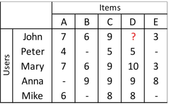
Figure 2.1 presents an example of a user-item matrix. We can see that there are a large number of unspecified values, which is common since each user only interacts with a small set of items. The following examples will explain each approach (user-based and item-based CF):

Example 2.1 - Query: How is John expected to rate item D?

▪ User-based CF: The goal is to find the user that rated items most similarly to John. Mary seems to rate items similarly to John, as both rated items A, B, C, and E in a similar, indicating that both may share similar preferences. Since Mary enjoyed item D (rating of 10), item D may represent a suitable recommendation to John.

▪ Item-based CF: The goal is to find the item, which other users rated most similarly to item D. Item C seems to share similar ratings to Item D. This may indicate both have similar characteristics. Since John enjoyed Item C, he is likely to enjoy Item D too.

Figure 2.1 Example of user-item matrix

Note: The presented example is illustrative to simplify the explanation of the concepts, without real calculations.

2.2.1.2. Explicit and implicit feedback

Given a set of m items and a set of n users, a CF system can construct an m X n matrix of user-item ratings. To correctly calculate similarities between users or items, we must ensure that the matrix is filled with meaningful values. The feedback that establishes the relationship between the users and the items can be either explicit or implicit (O’Bryant, 2017):

A

B

C

D

E

John

7

6

9

?

3

Peter

4

-

5

5

-Mary

7

6

9

10

3

Anna

-

9

9

9

8

Mike

6

-

8

8

-Items

U

se

rs

6 ▪ Explicit rating: consists of information feedback provided explicitly by the user on a specific item. An example of an explicit rating includes a one-to-five star on Amazon.com. On an online music streaming platform can be considered the Like Label assigned to a specific track. ▪ Implicit ratings: consist of information feedback inferred from the user’s behavior. An example

of an implicit rating can be the number of times a user visited the page of a specific product. On online music streaming platforms can be considered the play counts on a specific song. A song that was listened to many times would return a high implicit rating.

Although explicit feedback tends to be more accurate than implicit feedback, the first is scarce in the majority of the applications. Users do not always assign ratings to items, so RS cannot entirely rely on explicit feedback to recommend items to users. One of the current challenges that MRS is trying to tackle is the human effort problem. Generally, the more effort it takes for users to rate items, the fewer ratings they will provide. Since rating every song would result in a very dull task, it becomes essential to find ways to infer implicit feedback. The most common approach is to explore listening histories to understand which songs the user prefers the most. A song that has been played 100 times should have a higher rating than a song that has been played only 15 times (O’Bryant, 2017). Another example would compute the ratio of completed plays, for each user and item. A song that is often listened until the end should have a higher rating than a song that is often skipped. The inference of implicit rating is one of the current challenges that researchers are working on since better the inference of the rating, the better the accuracy of the RS.

2.2.1.3. Similarity measures between users and items

CF algorithms, firstly, determine the similarities between items/users to select the most similar items/users. Users or items can be displayed by vectors of fixed length, so this task is equivalent to calculating the similarity between vectors. The vectors contain values on the ratings of user-item information, and a similarity function is then applied. There are many different functions to compute the similarity between vectors. Among the most common ones, we will go through the Cosine similarity, Pearson correlation coefficient, and Jaccard Index (Sarwar, 2001):

▪ Cosine similarity: is calculated by computing the cosine of the angle between two vectors. In the context of ratings, similarity values range between 0 and 1, since no negative ratings are allowed. Higher the resulting value higher the similarity between the vectors. Given a m X n rating matrix, the similarity between items a and b be denoted as:

Cosine similarity (𝑎⃗, 𝑏⃗⃗)

=

‖𝑎⃗⃗‖‖𝑏⃗⃗‖

=

∑𝑛𝑖=1𝑎𝑖𝑏𝑖

√∑𝑛_𝑖=1𝑎_𝑖2 √∑𝑛_𝑖=1𝑏_𝑖2

,

(1)

where “ ∙ ” Denotes the dot-product of the two vectors.

▪ Pearson correlation coefficient: identifies which corresponding values in two vectors are positively or negatively correlated. The resulting value ranges from -1 to 1, where a similarity equal to -1 corresponds to an inverse correlation, and a similarity equals to +1 corresponds to a positive correlation. Before, we must isolate the cases where the users rated both 𝑖 and 𝑗.

7 Let the set of users who both rated 𝑖 and 𝑗 be denoted by U then the correlation similarity is given by: Person Correlation (𝑎⃗, 𝑏⃗⃗)

=

(2)

Cosine similarity measure has one critical drawback that we must take into consideration: in the case of user-based CF we calculate the similarity iterating through all users on the specific items, but in the case of item-based CF we only iterate through the items, accounting only one rating per user. So, calculating the similarity using cosine similarity in item-based case, the magnitude of the variability of ratings provided by each user is not taken into account. Sarwar, Karypis, Konstan, and Riedl (2001) describe the adjusted cosine similarity, an alternative measure which accounts for the corresponding user average rating for each co-rated pair, overcoming this drawback.

▪ Jaccard index: compares the similarity between two items. The goal is to calculate the percentage of times two items simultaneously occur out of the total number of times each one occurs. The Jaccard Index will output values ranging from 0, which means no similarity, to 1, which means maximum similarity. In RS a Jaccard Index of 1 would mean that two users would have rated the same items equally. Important to note that this measure is susceptible to outliers.

Jaccard Index

(𝑎⃗, 𝑏⃗⃗) =

(3)

2.2.1.4. Model-based Collaborative Filtering

In the last chapter, we went through the neighborhood-based techniques that can be seen as generalizations of the KNN algorithm, commonly used in semi-supervised learning problems. Neighborhood-based methods consist of generalizations of instance-based learning methods, in which the prediction approach is specific to the instance domain that we want to predict. In user-based methods, the neighbors of the target user are determined in order to perform the final prediction. However, this approach is hard to scale on large amounts of data. When dealing with an extensive catalog of items and a large set of users, Neighbor-based models may not be suitable due to the high processing time.

Often, it may be more suitable to build a summarized model of the data making recommendations more efficiently. Consequently, the prediction phase is isolated from the training phase and occurs in different moments. In order to reduce dimensionality and improve the efficiency of the model, matrix decomposition techniques are usually applied to the input data. These techniques try to capture the highest percentage of variability (explanatory power) possible while making an approximation of the user-item matrix and reducing the number of input variables.

The Single Value Decomposition (SVD) is a commonly used approach to decompose the user-item rating matrix. This operation decreases the complexity of the problem while reducing the

8 dimensionality. SVD decomposes the original matrix into three different matrices: U, 𝐷, and 𝑉𝑇_{, where}

the matrix U consists of the orthonormalized eigenvectors of 𝑅𝑅𝑇_{, the matrix V consists of the}

orthonormalized eigenvectors of 𝑅𝑇_{𝑅 and the matrix 𝐷 consists of a rectangular diagonal matrix with}

the non-negative square roots of the eigenvalues called singular value, sorted in descending order such that 𝐷1,1≥ 𝐷2,2, and so on. Higher the eigenvalue higher the importance of such latent factors. SVD

reduces the dimensionality of the original matrix by selecting the K-most important latent factors while preserving the maximum information possible.

Concerning the decomposed matrices, U contains features describing each user, D provides information about the importance of each element and 𝑉𝑇_{contains vectors with features describing}

the particular items.

Example 2.2: Let A be an 𝑛 X 𝑑 user-item matrix:

Α = 𝑈𝐷𝑉

₍₄₎

Figure 2.2 The SVD decomposition of an 𝑛 X 𝑑 user-item matrix

2.2.2. Content-Based Filtering Models

In the previous chapters, we explored CF systems that use latent information from user-item ratings to find patterns and to make recommendations. On the other hand, Content-Based Filtering (CB) systems focus on modeling the items being recommended by analyzing the characteristics of the users’ preferred items. CB recommender systems try to match users to items that are similar to what they have liked in the past. Therefore, the other users’ interests have little, if any, role to play in CB systems. CB systems are particularly useful to tackle the cold start problem when few ratings are available on a particular item or user. For instance, when a new song is released the volume of ratings may not be representative enough to recommend it. The same happens when a user has rated only a few items. Studies show that CB models do not need many users to provide relevant recommendations (O’Bryant, 2017).

In the context of MRS, CB recommendation relies on audio meta-data (e.g., genre) and audio signal analysis. Several ways were already proposed to generate audio attributes and metadata from the audio signal. Chou (2016), proposed a content-based system that analyzes audio signal files to determine song Features such as timbre, acusticness, and tempo. Another common approach is to analyze song files and assign tags by hand.

9 The process of using the CB algorithm to recommend an item involves two main tasks: information retrieval and information filtering. First, information on the item features are extracted through vector representation. Then, a CB profile is designed for each user based on the weighted vector of the item’s attributes. Cluster analysis, decision trees, artificial neural networks are some of the algorithms that can be used for the user profiling task. Finally, it is possible to arrive at an accurate recommendation by calculating the similarity distance between the users’ profiles and the items’ profiles.

Although RS using CB systems can provide useful recommendations quickly, overcoming the cold start problem, the effectiveness of those recommendations will not improve that much after the system gathered many users. The CB technique achieves this plateau because modeling users’ preferences may not contain valuable information on the items that the user does like or does not like. O’Bryant (2017) highlights that CB models record the users’ response towards each of the components in the item model (e.g., the gender of the vocalist). For instance, the model may indicate positive feedback towards songs with female vocals, so the user preference model will possibly indicate a positive bias concerning female vocals.

2.2.3. Hybrid Models

CF and CB methods have specific limitations that can compromise the accuracy and usefulness of recommendations. Hybrid methods emerged to overcome the limitations of using every single method as a separate piece. Instead, the two approaches can be combined into a holistic method that draws on the strengths of each. There are many different ways where both methods can be combined. O’Bryant (2017) proposed a method that uses CF as the default system, while CB filtering is used when the first lacks sufficient data about a particular item.

Burke (2002) proposes some combination methods that have been employed by researchers to combine different methods:

▪ Weighted: The recommended items result from the combination of the output results of the different recommendation techniques. The method mentioned above is a very straightforward approach where all of the system’s capabilities are carried together, being easy to perform post-hoc credit assignment and adjust the model accordingly. A possible approach may be to decrease the CF recommender impact for those items with a small number of rates.

▪ Switching: The recommended items result from switching between different recommendation techniques following some criterion and depending on the current situation. The benefit of a switching hybrid system is that it takes into account the strengths of each technique and the current conditions, so it can adapt whenever needed. This approach implies de determination of the switching criteria.

▪ Mixed: The recommended items result from using multiple techniques simultaneously. The recommendations of the different techniques are all presented to the user. The mixed approach avoids the cold start problem because the CB component can be relied on to recommend new items.

10 ▪ Feature Combination: The recommended items result from treating collaborative information as additional input features associated with each example and use content-based techniques over the final dataset. This approach lets the system consider collaborative data without relying exclusively on it, which reduced the system’s sensitivity to the number of users who rated an item.

▪ Cascade: The recommended items result from multiple stages processes where different techniques are applied. In this approach, one recommendation technique is applied first to produce a ranking of candidates, and then a second technique is applied to refine the recommendation from the set previously generated. Cascading systems only apply the second (or low-priority) technique on a smaller set of candidate solutions, which decreases the computational complexity. Additionally, this method allows the system to avoid employing the low-priority technique on items that already get well differentiated by the high-priority technique.

▪ Feature Augmentation: The recommended items result from incorporating the results of a first-applied technique into the second technique. The first technique generates a rating or a classification for an item, which is then processed by a second technique. In a Cascade hybrid, the second recommender does not use any output from the first recommend, while in Feature Augmentation, the second model uses the output of the first one.

▪ Meta-level: The recommended items result from using the model generated by a first technique as input for another technique. The meta-level technique differs from Feature Augmentation: in an Augmentation system, we use a learned model to generate input features to a second system; in a meta-level system, the entire model becomes the input.

2.2.4. Evaluation of Recommender Systems

Evaluating the performance of RS is one of the current challenges that researches and industry, in general, are trying to tackle. This challenge is mainly due to the high subjectivity that users’ tastes are subjected to, making it hard to understand in which situations users show empathy with specific songs. Nevertheless, there are standard metrics that are often used to assess models’ accuracy. In RS, the accuracy metric measures how close the rating predicted by the algorithm is to the real rating provided by the user.

One of the most used measures is the Root mean square error (RMSE), which consists of the difference between the predicted rating and the real rating. The Mean average error is a similar measure; however, it is more tolerant of high rating divergences. The lower both values are, the more accurate the model will be, and better recommendations will perform on real-life applications.

RMSE

= √

𝑛

∑

(𝑝

− 𝑟

)

11 MAE

=

𝑛

∑

|𝑝

− 𝑟

|

𝑖=0

(6)

Another widely used measures to evaluate the performance machine learning models are Precision and Recall. They are introduced in RS domain applications by Sarwar (2000). When the model recommends to the user with a list of items, those items can be classified as relevant (if the user liked them) or irrelevant (if the user did not like them). On the other hand, the items that were not recommended to the user can also be classified as relevant (if the user did not like them) or relevant (if the user liked them). Precision consists of dividing the relevant items that were recommended to the user by the total number of items in the recommendation list. Recall consists of dividing the relevant items that were recommended to the user by the total number of relevant items available.

Precision

=

𝑟𝑒𝑙𝑒𝑣𝑎𝑛𝑡 𝑖𝑡𝑒𝑚𝑠 𝑟𝑒𝑐𝑜𝑚𝑚𝑒𝑛𝑑𝑒𝑑 + 𝑖𝑟𝑟𝑒𝑙𝑒𝑣𝑎𝑛𝑡 𝑖𝑡𝑒𝑚𝑠 𝑟𝑒𝑐𝑜𝑚𝑚𝑒𝑛𝑑𝑒𝑑

(7)

Recall

=

12

3. CURRENT CHALLENGES IN MUSIC RECOMMENDER SYSTEMS RESEARCH

In this chapter, we go through what we believe to be the most critical challenges in MRS research, describing in detail the several standard practices, as well as its restrictions. Additionally, since some music-related characteristics have a direct impact on the challenges, we also provide context on the significant aspects and particularities of music recommendation.

3.1. P

M

C

As we have mentioned previously, there are some particularities on music consumption that makes music recommendation a particular topic. These characteristics and particularities make it hard to compare MRS to other RS, such as recommending books or movies. Schedl (2018), propose several music-related aspects that should be considered when building an MRS:

▪ Duration of items: Most of the RS recommends items that are consumed or purchased as an isolated act. If we consider the movie recommendation, the typical duration of a movie is 90 minutes. On the other hand, the average duration of music items ranges from 3 to 5 minutes, which makes music items more disposable compared to other items.

▪ The magnitude of items: The size of music catalogs tends to be more extensive when compared to other items. We can hypothesize that there are more music items on Spotify than movie items on Netflix. This large magnitude of music items makes scalability a much more important issue than in movie recommendation.

▪ Sequential consumption: Unlike movies, usually music is consumed sequentially. It is not very common a person to watch several movies in a row, perhaps, due to the higher duration. In contrast, rarely a person listens to one song at a time. Therefore, identifying the right arrangement of items in a recommendation list becomes critical.

▪ Recommendation of previously recommended items: In music consumption, there is a propensity for the user to listen repeatedly to some specific songs. Having said so, we should not discard recommending an item that has already been recommended in the past. This behavior contrasts with movies or books recommendation because people tend not to repeat this kind of item.

▪ Consumption behavior: When using implicit feedback (i.e., listening logs), to infer the listener preferences, we should consider that it may contain bias, since music is often consumed passively, in the background (i.e., studying).

▪ Listening intent and purpose: Users may have different motivations and purposes when listening to music. Studies found that the type of music users listen to when they alone differ from the kind of music they listen to when they are with friends. The same happens when people are sad and listen to music as a mood regulator (Schäfer, 2013). That introduces noise

13 when trying to unveil the real users’ preferences. A perfect MRS would consider these purposes and recommend accordingly.

▪ Emotions: Emotions are known to play an essential role in music preferences, perhaps because music tends to invoke strong feelings. We can hypothesize that emotions have a direct influence on recommendations accuracy. Music recommendation driven by emotions is an active research area, where tracks are tagged according to emotional terms.

▪ Listening context: Music preferences are highly dependent on users’ situational and contextual aspects. For example, a user may listen to a different playlist when preparing for a romantic dinner than when warming-up to go out with friends on a Friday night. Situational-aware MRS is a current research area, taking such contextual factors into account when recommending music.

3.2. C

M

R

S

Bearing in mind all these music-related aspects mentioned above, which have a direct or indirect impact on the current challenges of MRS, we now identify and describe a selection of challenges, which we believe the industry of MRS is currently focused on overcoming. Not being able to touch all challenges exhaustively, we focus on cold start problem, evaluation, popularity bias, and over-specialization.

3.2.1. Cold start Problem

The cold start problem is directly impacted by the data sparsity problem, which refers to the fact that the number of provided ratings tend to be much lower than the number of possible ratings. So, the problem becomes even more critic when the user-item matrix increases in size, meaning that higher the sparsity of the matrix, lower the rating coverage. Having said so, we can conclude that online applications like Spotify, which makes available almost all the music in the world, the cold start problem becomes a central issue to tackle when recommending music to users.

Researchers proposed many approaches to tackle the cold start problem in the field of MRS. These approaches rely on the utilization of content-based approaches, hybridization, cross-domain recommendation, and active learning.

As we previously mentioned, CB techniques can overcome the new item problem, when few ratings are available on a specific song since they do not rely on song ratings but rather on the song’ descriptors as a basis for the recommendation (Aggarwal, 2016). An alternative approach to tackle the new item problem is to combine CB and CF into a hybrid model that uses the strengths of each model whenever it is appropriate (Schedl, 2018). Cross-domain recommendation techniques can also be the right approach when tackling the cold start problem by making use of information about users’ preferences, by transferring information from an auxiliary domain to the music domain (e.g., User personality). Finally, active learning addresses the cold start problem at its origin by quickening the process of finding the user’s preferences by exploring areas of the catalog that the user has not seen.

14 Aggarwal (2016), explains that active learning methods ask the user to rate specific item combinations while giving the recommendation system better accuracy.

3.2.2. Evaluating Music Recommender Systems

When building an RS, it becomes essential to find ways to assess the quality of the recommendations that models provide to the users. The field of RS borrowed the most used evaluation metrics from machine learning and information retrieval standard practices. Accuracy metrics, such as precision and recall, are the most commonly used criteria to assess the recommendation quality of an RS. However, new measures that are more appropriate to the recommendation problem have emerged in recent years. These take into account the core characteristics of MRS such as utility, novelty, and serendipity. However, these metrics integrate abstract factors that become hard to describe from a mathematical point of view.

The most frequently used performance measures can be roughly categorized into accuracy-related measures (i.e., mean absolute error), standard information retrieval measures (i.e., precision) and beyond-accuracy measures (i.e., diversity). Also, to assess the system’s ability to position suitable recommendations at the top, it became essential to adapt some of these metrics to consider the ranking position of the items (i.e., precision at top K recommendations). Figure 3.1 describes some recently proposed measures to assess the quality of recommendations.

The common practice when measuring the performance of an RS consists of comparing new results against existing datasets. Given a dataset of human listening history, one or more songs are removed from the dataset. Then, the test dataset is given to an RS, and the system generates a list of suitable recommendations to provide to the end-user. The performance measures are frequently based on how often the system can pick the same songs that were removed previously from the original listening history.

Despite the improvements in MRS evaluation strategies, the user factor is still a challenge not adequately addressed by the current practices. For instance, while several proposed quantitative measures like serendipity and diversity, the users’ perception can highly differ from the measured ones. This difference means that even with beyond-accuracy metrics, RS cannot fully capture the real user satisfaction. Instead, approaches based on the UX of online streaming platforms can also be explored to evaluate RS. For instance, an MRS can be evaluated, taking into account user engagement, which may provide useful insights about the relevance of the recommendations.

15 Figure 3.1 Evaluation measures commonly used for RS (Schedl, 2018)

3.2.3. Popularity Bias

An additional current challenge in MRS is the popularity bias that results from the significant preponderance that CF techniques give to popular items (those with more play counts or ratings) over other “long-tailed” items that may only be popular among small groups of users. Although in the majority of the cases recommending a popular song might result in a good recommendation, delivering only popular songs will not enhance the overall experience of the user, ignoring more specific song interests that users might have. It also means that the model could be biased towards more famous artists, disadvantaging producers of less popular songs. Since, recommending serendipitous items from the long tail is generally considered an essential characteristic of recommending items, popularity bias increase the chance that users will hear songs that they already know. Additionally, systems currently using active learning to explore users' preferences will typically explore new search spaces, finding items the user is less likely to know about and where the system will gain more insights about the users' real preferences (Resnick, 2013).

Figure 3.2 illustrates the long-tail phenomenon in MRS proposed by Abdollahpouri (2019). The y-axis represents the number of ratings per item, and the x-axis represents the rank of the recommended item. The first vertical line separates the top 20% of the items by popularity – short head items. Cumulatively, this 20 % has many more ratings than the remaining 80% of items to the right. The second vertical line divides the tail of the distribution into two parts. The first part is called long-tail, where belong items that can rely on CF techniques, even though many algorithms fail to position them in the top recommendation lists. The right part represents the items that receive so few ratings that become unreliable to recommend to a user – distant tail. In these cases, as we covered, different techniques may tackle it.

16 Figure 3.2 The long-tail of item popularity (Abdollahpouri, 2019)

3.2.4. Over-Specialization

Being novelty one of the critical aspects of recommendations, RS must consider it when recommending items. When the RS does not achieve novelty, items will tend to be similar to what the user has already seen. This similarity suggests that the algorithm is starting to get over-specialized. When a user gives positive feedback to several items (through a rating for example) that are someway similar to each other, the system creates a positive connection between the item category and the user (this connection is abstract and happens automatically). So, the algorithm may start to get overspecialized in that items’ category. When the recommendation algorithm becomes overspecialized, it only recommends songs from the categories the user has listened in the short past. At first, this might look positive since the users receive recommendations related to items they enjoyed. Since no connections were established with other item-groups, the user will not get diversified recommendations. One of the current approaches to tackling the problem of over-specialization is to include random items on the recommendation list. By doing so, the system will able to broaden the perception of users’ preferences while ensuring novelty at the same time.

17

4. RELATED WORK

Researchers led several studies on RS over the last decade. In this Chapter, we go through some of the research topics that provided positive contributions to the field of RS. Furthermore, we present and describe in more detail some of the work projects on MRS, that we consider relevant to the development of this dissertation.

4.1. R

S

RS has become an essential part of the academic literature domain due to the increasing contribution of improvements in the study field since the emergence of the first paper introducing CF approaches in 1990. n 1992, Xerox Palo Alto Research Centre developed the first real RS application. The system was named Tapestry, and it was based on a simple CF approach to filter the volume of incoming mail, which by that time was huge due to the increasing use of electronic mail (Huttner, 2009). Over the last decade, researchers have been focused on improving CF and CB techniques on real-life applications. Although, these research studies are often focused on specific domains of RS development, like music or movies, being influenced by the particular aspects of the respective domain.

As RS has become a more complex field, different survey papers have been released. The current research studies on RS mainly focus on combining different methods into hybrid adaptive models, creating new performance measures to better assess RS' quality, and decrease the computational cost of running such complex models. Among the earliest published research papers on RS, a hybrid system architecture has been proposed by Burke in 2002 and 2007. Adomavicius (2005) conducted a survey presenting the limitations of CF, CB, and hybrid techniques, including possible improvements in RS. Shani (2011), focused on the efficiency and effectiveness of RS by proposing a list of different measures to better assess the accuracy and performance of the models. Bobadilla (2013), presented a survey mainly focused on CF techniques while summarizing the context evolution of RS alongside with the web developments in recent years. Although recent research studies are helping to develop and improve the RS field, further progress is still needed for RS to be efficient and overcome the main challenges that real-life application problems trigger.

4.2. M

R

S

The first research study on music recommendation was released in 1994 (Shardanand, 1994), but more studies emerged from 2001 on, with the increasing use of online streaming platforms (Celma, 2010). Nowadays, thanks to the higher penetration of music streaming services like Spotify and Apple Music, such platforms give their users access to vast catalogs of music pieces, growing in size with new songs released every day. Although MRS techniques have shown often good results when suggesting songs that fit users’ preferences, these systems frequently produce unsatisfactory recommendations, leaving some room to improve. In this chapter, we go through some of the past research studies in the field of MRS. The main objective of the more recent developments in the industry is to overcome and mitigate the challenges that these systems currently face. The current research studies are directly related to the current challenges that have already been presented in the previous chapter.

18 Since 2005, that research the community is trying to find alternative approaches to pure CF and CB techniques, broadening its attention to new techniques. The current research studies are mainly centered on topics such as hybrid methods, automatic playlist continuation approaches, and new evaluation methodologies.

Jannach (2015), proposed in their research study a multi-aspect scheme that combines patterns in the listening history with metadata features and personal user preferences to achieve better performance. This hybrid application uses a post-processing procedure to better match the characteristics of the most recently played songs.

O’Bryant (2017), proposed an offline hybrid system that uses active learning and CB techniques to become more resistant to the cold start problem. The system explores users’ existent collections (i.e., users’ library) and by recording and tracking the skipping behavior on songs belonging to those collections can accurately recommend the next track to be played – next-track recommendation. By recording the skipping behavior on songs that the users listen becomes possible to identify those tracks that the user did not want to listen at a specific time. Moreover, the approach of using skipping behavior as the evaluation metric of the system places the user at the center of the evaluation process. According to a study carried by the Music Business Association in 2016, playlists accounted for 31% of music listening time among listeners in the USA. Additionally, by the end of 2018, Spotify was hosting more than three billion user-created playlists (Newsroom Spotify, 20181_{). All these insights suggest}

that playlists are becoming people’s preferred way to listen to music. Thus, some research studies have been focused on the task of automatically extend existent playlists by suggesting one or more tracks to be added to it, while preserving the core characteristics of the original playlist – Automatic Playlist Continuation (APC). APC helps users to listen to music continuously while also decreasing the amount of user effort involved in the process. In some recent approaches, the target characteristics of the playlist are specified by a set of musical attributes or metadata such as timbre, tempo, artist, and others. In more recent approaches, the playlist might be extended given a single seed track or given a start and an end song. Other systems, focus on smooth transitions, ensuring smooth transitions so that sequential songs are as similar as possible Schedl (2018).

Vall (2018), investigate the impact of the song context and the song order on next-song recommendations by conducting offline experiments. Their output results indicated that the song context has a positive impact on next-song recommendations, but, on the other hand, the song order did not appear as a significant variable when recommending the next song to play.

Researchers have released different datasets that can be used to train and evaluate models on music recommendation. The Last.fm dataset provided by Celma (2010), contains listening information for about 360 thousand users, including only the artists they listen more frequently to. Moreover, each listening event registers the respective artist and the track name. Another well-known dataset is the Million Song Dataset (MSD) being possibly one of the most widely used datasets on MRS’ research. The dataset makes available information on the audio content descriptors of each song, user-generated tags attributed to songs, term vector representations of lyrics, and the respective play count

19 by each user. A sample of the Last.fm dataset will be used throughout this dissertation to build the RS and to assess the performance of the model.

20

5. METHODOLOGY

As we already reported, recommending the right music to the right user might be considered as one of the critical success factors of music online streaming services. The experiments that we will conduct throughout the following chapter aim to propose a CF methodology to recommend songs that match users' preferences accurately. This section, also, focuses on presenting the results of the proposed system, while comparing the respective results with another baseline model. Furthermore, we will outline the data acquisition procedure, describe the dataset, by analyzing the variables, and presenting some basic descriptive statistics.

5.1. I

All the models and experiments were implemented in Jupyter Notebook environment using Python programming language. Several packages were used to help to develop the model and processing the dataset. We highlight Scikit-learn2 _{used to develop the models and Pandas}3 _{to process and clean the}

dataset. We ran all the experiments on a MacBook Pro with Intel Core i5 CPU and 8 GB RAM and MacOS operating system.

5.2. P

C

Before going further on the methodology report, we should draw some preliminary considerations that support the project:

▪ One of the critical aspects of CF models is the greater the volume of data available, the higher the accuracy of the RS. However, the model will have to process large amounts of data, requiring significant computation power. This limitation will result in a substantial amount of time to run the model. Having said so, we have decided to use a subset of the data, while ensuring interpretability allowing us to evaluate its performance;

▪ The data that will be used to build the RS represents real-life listening histories from real users. However the data is entirely anonymous, and each user is only identified by a unique primary key protecting their identity;

▪ The data that will be used to build the RS dates back to 2011. Thus, we should take into account that the most popular songs in the dataset may not be aligned with today's reality.

2_{https://scikit-learn.org/stable/} 3_{https://pandas.pydata.org/}

21

5.3. I

In the development of this dissertation, we used a subset of data from the Million Song Dataset (MSD), which was provided by The Echo Nest in 2011. The dataset contains two different files:

▪ User information: contains information on the user_id, the song_id, and the listen_count of the particular song:

Table 1 User information dataset file

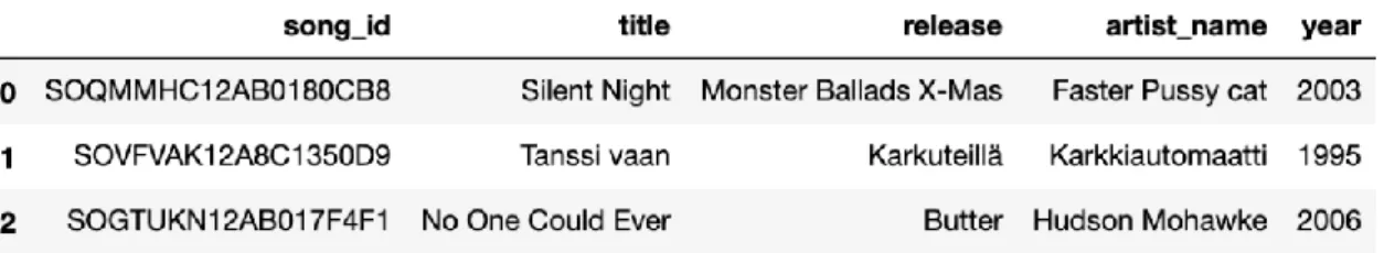
▪ Song information: contains information on the song_id, song_title, artist_name, and realed_year (if available):

Table 2 Song information dataset file

5.3.1. Data preprocessing

As a matter of convenience, we integrated the information of both datasets into a single file to access the complete information and simplify the data manipulation pipeline. Moreover, the entire dataset contained 2 000 000 observations. Thus, it would be too time-consuming to download it entirely to the local machine. Having said so, to manipulate and process the data efficiently, we extracted a subset of 10 000 songs from the original dataset. Table 3 shows a sample of the final dataset, and Table 4 provides the metadata for each attribute.

22 Table 3 Final dataset sample (n=10)

Table 4 Attributes and respective metadata

There is no much information that can be extracted from the dataset since the data formats only allow us to calculate some simple counts. Although, in order to better understand the data and the problem context, we compute some basic descriptive statistics that may be relevant:

▪ 365 total number of unique users; ▪ 5 151 total number of unique songs; ▪ 1 994 total number of unique artists; ▪ 3 103 total number of unique albums; ▪ 29 911 total number of plays counts.

Based on these statistics, we can conclude that on average, each user listens to 14 different songs and five different artists. Also, since the total number of plays is higher than the number of songs, it means that users are listening to songs repeatedly. This notion of listening songs more than once is essential to introduce the concept of music popularity. We may hypothesize that songs with greater play counts are more popular among others. Having said so becomes necessary to identify the popular songs in the dataset. For that purpose, we create a new variable that calculates the percentage of play counts for each song. Then, we list the 15 most popular songs in the dataset, as shown in Figure 5.4:

Variable Description

user_id Primary key to identify each user

song_id Primary key to identify each song

listen_count How many times a user listened a specific song

title The respective song's name

release The respective album's name

artist_name The respective artist's name

23 Table 5 Top 15 popular songs

By observing Figure 5.4, it is possible to conclude that Harmonia from Sehr Kosmisch is the most popular song accounting for 0.45% of the total amount of play counts.

5.4. U

The RS must be able to predict whether a specific item should be recommended to a given user. Our system is based on a CF technique that uses the KNN algorithm to recommend the top items more likely to fit users' preferences. In order to have a baseline model to compare results from different models, we will evaluate two different RS techniques: CF approach using the KNN algorithm and a Popularity-based Model. We go in detail about the specifications of each model in the following chapters.

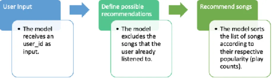
5.4.1. Popularity-based model

The Popularity-based model recommends items based on a very simplistic approach. As we already reported, recommending popular songs to users is likely to result in an accurate recommendation, but this approach does not focus on the real user' interests. The model operates independently from the user preferences and will always recommend songs by just ranking them according to their popularity. In order to compare the results and to have a compare baseline, we developed a Popularity-based model. The Popularity system outputs a list of k (parameter) songs sorted by how frequently that song has been played for all users. Then, we recommend a list of songs that the user has not listened to yet.

24 Figure 5.1 Popularity-based Model Framework

5.4.2. CF Model

Popularity-based models may output the same recommendations to independently of the users because the listening history of the users does not take a role in the process. On the other hand, the CF model overcomes this issue by taking into account the preferences of each user, recommending personalized songs accordingly. Instinctively, if two songs often appear together in the users' listening histories, we may hypothesize that those songs share some level of similarity. Having said so, they are also likely to appear together when recommending a list of songs to a user. Based on that assumption, the model makes recommendations by finding songs that are similar to each other, based on the users' past listening history. We are trying to answer the question: For a particular song, how many times users, who listened to that song, also listen to another set of other songs.

Item-item filtering approaches require the implementation of a co-occurrence matrix based on the songs the users listen to. Given a user: The user's history songs get arranged along the length, and every song in the dataset gets arranged along the width; Then, the co-occurrence matrix gets populated by calculating a similarity score for each (item, item) pair. We used the Jaccard Index measure to calculate the percentage of times that two songs belong to the same listening history out of the total times each one belongs to any listening history. The scores get sorted descending, and the top k (parameter) recommendations are selected to provide the recommendation to the final user.

25 It is important to note that when using the CF approach, the co-occurrence matrix will tend to be very large. This large dimension will not be compensated by higher information since the co-occurrence matrix will tend to be very sparse (null values for several item-item intersections). Data sparsity is due to the fact that there several songs that never listened to together. As we already covered, data sparsity is one of the critic challenges in RS in general, often resulting in additional computational costs.

5.5.

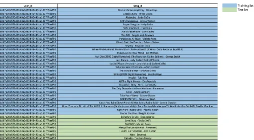
In order to compare the performance of both models, we provided a common data schema for each technique. To split the dataset into train and test sets, we used the function train_test_split from Scikit-learn4 _{package. The first subset (training set) is used in the training phase, representing 80% of each}

user listening history. The second subset (test set) is hidden during training and is only used later for the evaluation of both models. Figure 5.6 illustrates the data split process for each user. From now on, we will use the user_id "dd67a78d5f9d8140a0d83849441ca1807f7ea790" to useful examples.

Table 6 Example of listening history train/test split

To recommend the top songs to the respective users, we use the KNN algorithm. The KNN algorithm uses the user-defined parameter k to select the top songs to recommend. The definition of parameter k has a high impact on the model's performance. Greater the k higher will tend to be the performance measures (precision and recall). Ultimately, we could list the entire list when recommending the songs to the user, ensuring that the hidden songs belonging to the user listening history are there. However, since we want to evaluate the ability of the models to list the most relevant songs first, we should keep the number of parameter K relatively small. In other words, we want a model to be able to output as many relevant songs as possible in a few recommendations. We decided to use k=10 because it is one of the best practices among different online music streaming platforms (i.e., Spotify).

4_{https://scikit-learn.org/stable/}

26

5.6. P

E

In this chapter, we will output recommendations by using each model separately, in order to understand, from a practical point of view, which one tends to perform better. Although this is a very naïve approach, it may be useful to understand the specificities of each model better, and their overall performance, as well. To achieve this, we will extract a random user from the dataset: user_id: dd67a78d5f9d8140a0d83849441ca1807f7ea790. So, in Table 7, we present the entire listening history of the user_id mentioned above.

Firstly, we provide both models with the training set (Table 8), and we run both to produce recommendations. Then, we draw some conclusions from the recommendations provided by each model to understand which one achieved better results. It is important to note that our objective is to output the songs that are present in the test set (Table 9) because these are the ones that are "hidden" in the training set.

27 Table 7 Training Set Example

Table 8 Test Set Example

5.6.1. Popularity-based Model vs. CF-based Model

Table 9 Popularity-based Model Recommendations

User_id Song_id

dd67a78d5f9d8140a0d83849441ca1807f7ea790 Doesn't Mean Anything - Alicia Keys

dd67a78d5f9d8140a0d83849441ca1807f7ea790 Greece 2000 - Three Drives

dd67a78d5f9d8140a0d83849441ca1807f7ea790 Alejandro - Lady GaGa

dd67a78d5f9d8140a0d83849441ca1807f7ea790 Filthy|Gorgeous - Scissor Sisters

dd67a78d5f9d8140a0d83849441ca1807f7ea790 Paper Gangsta - Lady GaGa

dd67a78d5f9d8140a0d83849441ca1807f7ea790 Sehr kosmisch - Harmonia

dd67a78d5f9d8140a0d83849441ca1807f7ea790 Ain't Misbehavin - Sam Cooke

dd67a78d5f9d8140a0d83849441ca1807f7ea790 The Gift - Angels and Airwaves

dd67a78d5f9d8140a0d83849441ca1807f7ea790 Parabienes Al Reves - Violeta Parra

dd67a78d5f9d8140a0d83849441ca1807f7ea790 I Don't Feel Like Dancin' - Scissor Sisters

dd67a78d5f9d8140a0d83849441ca1807f7ea790 Revelry - Kings Of Leon

dd67a78d5f9d8140a0d83849441ca1807f7ea790 When We Murdered the World on the Fourteenth of May - Ordo Rosarius Equilibrio

dd67a78d5f9d8140a0d83849441ca1807f7ea790 Make Love To Your Mind - Bill Withers

dd67a78d5f9d8140a0d83849441ca1807f7ea790 Nut City (2000 Digital Remaster) (The Rudy Van Gelder Edition) - George Braith

dd67a78d5f9d8140a0d83849441ca1807f7ea790 Just Dance - Lady GaGa / Colby O'Donis

dd67a78d5f9d8140a0d83849441ca1807f7ea790 Lucky (Album Version) - Jason Mraz & Colbie Caillat

dd67a78d5f9d8140a0d83849441ca1807f7ea790 Whataya Want From Me - Adam Lambert

dd67a78d5f9d8140a0d83849441ca1807f7ea790 The Invisible Man - Michael Cretu

dd67a78d5f9d8140a0d83849441ca1807f7ea790 Unite (2009 Digital Remaster) - Beastie Boys

dd67a78d5f9d8140a0d83849441ca1807f7ea790 Invalid - Tub Ring

dd67a78d5f9d8140a0d83849441ca1807f7ea790 All The Right Moves - OneRepublic

dd67a78d5f9d8140a0d83849441ca1807f7ea790 Beautiful_ Dirty_ Rich - Lady GaGa

dd67a78d5f9d8140a0d83849441ca1807f7ea790 The Only Exception (Album Version) - Paramore

dd67a78d5f9d8140a0d83849441ca1807f7ea790 Fever - Adam Lambert

dd67a78d5f9d8140a0d83849441ca1807f7ea790 Take Your Mama - Scissor Sisters

dd67a78d5f9d8140a0d83849441ca1807f7ea790 ROCKSTAR 101 - Rihanna / Slash

dd67a78d5f9d8140a0d83849441ca1807f7ea790 Catch You Baby (Steve Pitron & Max Sanna Radio Edit) - Lonnie Gordon

dd67a78d5f9d8140a0d83849441ca1807f7ea790 Horn Concerto No. 4 in E flat K495: II. Romance (Andante cantabile) - Barry Tuckwell/Academy of St Martin-in-the-Fields/Sir Neville Marriner

dd67a78d5f9d8140a0d83849441ca1807f7ea790 Right Now (Radio Edit) - Atomic Kitten

dd67a78d5f9d8140a0d83849441ca1807f7ea790 You're The One - Dwight Yoakam

Training Set

User_id Song_id

dd67a78d5f9d8140a0d83849441ca1807f7ea790 Bring Me To Life - Evanescence dd67a78d5f9d8140a0d83849441ca1807f7ea790 Love Story - Taylor Swift dd67a78d5f9d8140a0d83849441ca1807f7ea790 FANTASY - Mariah Carey dd67a78d5f9d8140a0d83849441ca1807f7ea790 Mercy:The Laundromat - Pavement dd67a78d5f9d8140a0d83849441ca1807f7ea790 I CAN'T GET STARTED - Ron Carter dd67a78d5f9d8140a0d83849441ca1807f7ea790 Halo - Beyoncé dd67a78d5f9d8140a0d83849441ca1807f7ea790 Canada - Five Iron Frenzy