Ecosystem service assessment for urban planning: a French case study Pedro Cabral1,5, Harold Levrel2, Clément Feger3,4, Mélodie Chambolle4, Damien Basque4
1 Université de Brest, UMR AMURE - Centre de droit et d'économie de la mer, IUEM, 12 rue du Kergoat, CS 93837, 29238 Brest Cedex 3, France, Corresponding author, Email: [email protected]
2 Ifremer, UMR AMURE, Unité d'Economie Maritime, BP 70, F-29280 Plouzané Cedex, France 3 Muséum National d’Histoire Naturelle, UMR 7204 – CESCO, Paris, France
4 LyRE, centre de recherche de Lyonnaise des Eaux Bordeaux, France 5
Instituto Superior de Estatística e Gestão de Informação, ISEGI, Universidade Nova de Lisboa, 1070-312 Lisboa, Portugal
Abstract
Ecosystems provide a varied range of services to people known as ecosystem services (ES) which contributepositively to human well-being. Thus, their quantification and integration into planning decisions has become increasingly important.In this study we analyzed ES provided by the landscape of the Urban Community of Bordeaux (CUB) in France. These ES were selected using a participatory approach with local stakeholders and involved the creation of scenarios of land use and cover change (LUCC) expressing alternative planning options. Only open data was used. Results show that allthe analyzed ES, except erosionregulation, have decreased as a consequence of LUCC between 1990 and 2006. For year 2030, the "Plan" scenario, which integrates approved urban local plans, is the one that will cause more negative impacts on the CUB ES. Both "Conservation" scenarios present a more balanced situation allowing to choose between carbon storage improvement or agriculture preservation with a degradation on nitrogen and phosphorous retention ES. We also found that there is little or no tradeoff on nutrient and sediment retention services regardless of the scenario used. This spatial explicit approach to ES modeling enables an informed discussion with the stakeholders about different planning options and their impact on ES and tradeoffs. Additionally, it may be used to effectively implement, monitor and communicate planning policies.
Key-words: ecosystem services;geographical information systems; spatial planning;land use and cover change models; open data
1. Introduction
Ecosystems are increasingly subject to multiple human uses and pressures which may compromise their ability to deliver ecosystem services (ES)necessary to support mankind (Halpern et al., 2007; Harley et al., 2006). The research field on ES which emerged on 1970s at the intersection of research in ecology and economy (Meral, 2012) is now flourishing and the number of articles on this subject continues to grow (de Groot et al., 2012; Jeanneaux et al., 2012; Vihervaara et al., 2010). ES approaches are seen by many as a promising way to better take into account the ecosystems in the decision process because they seek to make visible the multiple contributions of nature to society and associated tradeoffs (Goldstein et al., 2012; Tallis and Kareiva, 2006). However, this field is alsocrossed by controversyfocusing, particularly, on the definitions and methods of classification of ES(Boyd and Banzhaf, 2007; Fisher et al., 2009; Gatzweiler, 2006; Nahlik et al., 2012), on the development of biophysical and economic valuation methods (Chevassus-au-Louis et al., 2009; Lamarque et al., 2011; Nelson et al., 2009).Given the growing popularity of this concept, initially forged to draw attention on the importance of multiplying efforts to conserve ecosystems, it is now important to test on the field the effectiveness of such an approach and associated tools so that their ability to be included in the decisional process in practical management situations at the territorial level can be assessed.Therefore, quantitative assessments are of great importance to acknowledge the value of ES that otherwise would tend to be ignored by land use planners (Nelson et al., 2009). Knowing the impacts of land use management practices on ES production is crucial for an effective design of policies that will ensure the provision of the desired ES (Nelson et al., 2009). It has also been reported that the effective use of ES knowledge benefits from meaningful stakeholder participation, scenario development and the integration of local and traditional knowledge (McKenzie et al., 2014).
A variety of tools have been recently developed to integrate ES in the decision process. They seek more systematic approaches to ES, i.e., to make more quantifiable and reproducible assessments and to respond to various issues and contexts of decision-making (Bagstad et al., 2013; Peh et al., 2013). These tools range from simple spreadsheets (WRI, 2012) to sets of complex spatial modeling software (Bagstad et al., 2011; Feng et al., 2011; Tallis et al., 2014). They differ in data requirements as well as on the time andeffort to complete the assessment. Some are applicable to any place on the planet and are adapted to national or regional scales (Bagstad et al., 2011), while others are site-specific and limited to someES(Parametrix, 2010; Peh et al., 2013). Some favor the biophysical assessment of ES(Bagstad et al., 2011; Tallis et al., 2014) while others also offer monetary valuations (EVT, 2012; Tallis et al., 2014). Finally, these tools also differ in how to involve stakeholders in the study area.
In this paper, we report the results of a spatial explicit and participatory approach to assess in an integrated way multiple ES using InVEST models and other own produced indicators with open data. The objectives are: (i) to describe the evolution of ES in the CUBusing a time series of land use and land cover (LULC) between 1990 and 2006; and to (ii) anticipate plausible scenarios for year 2030 to understand howLUCCimpacts ES and tradeoffs. Results are expected to contribute to the definition of CUB urban planning instruments.
2. Data and methods 2.1 Study area
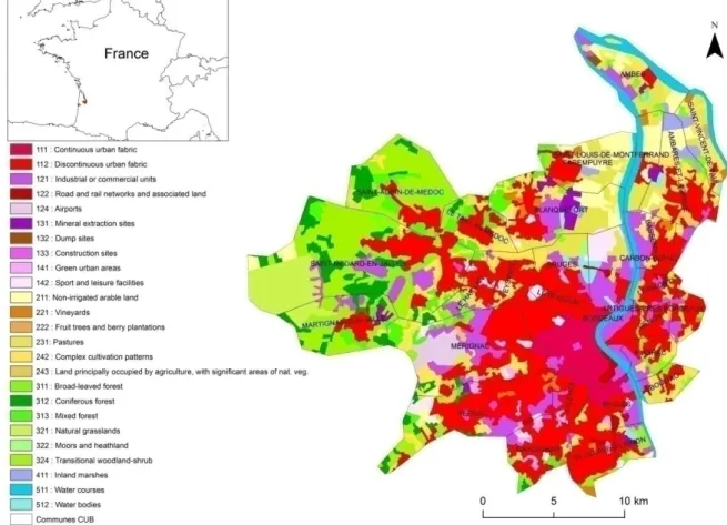
The CUB is composed of 28 administrative areas (Communes) and has about 57632 ha (Figure 1). It has a varied LULC composition including densely urbanized areas, agricultural and vineyard areas, the Landes forest on the NW and important wetlands along the river La Garonne. It is an area characterized by low slopes and low elevation (< 105m). The context of the study area is interesting because it presents a set of practical issues in land use planning related with the CUB expectation of reaching one million inhabitants by 2030 (727,256 inhabitants in 2011). To manage this expectation the CUB launched, in 2009, a prospective approach that resulted in a policy document, the "Metropolitan Project", which articulates a vision for the city to year 2030. Among others, the "55000 ha for Nature" initiative aims to make compatible the demographic growth with the "respect and valuation of the natural spaces in the city, the well-being and the respect for the biological needs of plant and animal species"(CUB, 2012). The CUB therefore wishes to put the "collective relationship to nature" at the heart of its reflection in the coming decade. The willingness to better account nature in the metropolitan project has also resulted in planning instruments such as the SCoT (Schéma de cohérence territoriale) or the PLU (Plan local d'urbanism). Thus, the quantitative spatial assessment of ES of the territory may help attaining these objectives.
Figure 1 The CUB and land use and land cover in year 2006 (Data sources: EEA, 2006 and IGN, 2012)
2.2 Project development approach
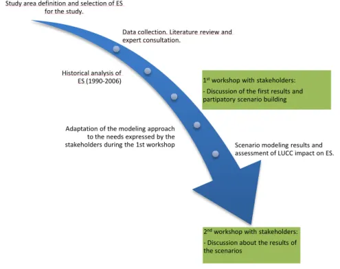
This 2-year project started with the selectionof the relevant ES with the help of the stakeholderswhich included representatives of the Aquitaine region, several environmental ONG, the agriculture chamber, a water company and CUB department's of water, nature and urbanism (Figure 2).Data collection activities and
anextensive literature review about values of parameters required to run the ES models was carried out. Local scientific experts were consulted for the cases in which we did not find any adequate values in the literature.
An historical analysis of ES level between 1990 and 2006was carried out and presented to stakeholders in the 1st workshop in the end of the first year of the project. During this workshop, remarks were made about the usefulness of some indicators and the way they were communicated. For instances, changes were made to the recreational indicator (access to green and blue areas) that did not consider urban sprawl and demographic growth aspects. It was also found that it would more useful report results using the administrative areas instead of the sub-watersheds.Future plausible scenarios that translated the CUB planning challenges were also discussed for year 2030 during this workshop.The use of consistent scenarios for potential future states that represent policy-induced changes to services integrating coherent narratives are more informative than the ones solely based on gross estimates (Peterson et al., 2003; Raskin, 2005; Swetnam et al., 2011).
The final workshop, in the end of the 2nd year, was dedicated to sharing the results of the scenarios and to discuss the possible use of the results for influencing planning decisions.
Figure 2Workflow of this study
2.3 ES models and biophysical indicators for the CUB
The selected ES were assessed using InVEST models (InVEST, 2013)together with own produced indicators.These are deterministic models which use a variety of spatial data, including LULC and biophysical data in the form of tables of coefficients(Tallis et al., 2014). They are based on ecological production functions that define how the spatial extent, the structure and functioning of ecosystems, the LULC and the intensity of human activities and uses of natural environments determine the local production of ES. These models produce three main types of results: quantitative results (biophysical), cartographic representations and, in some
Study area definition and selection of ES for the study.
Data collection. Literature review and expert consultation.
Historical analysis of
ES (1990-2006) 1stworkshop with stakeholders:
- Discussion of the first results and partipatory scenario building
Adaptation of the modeling approach to the needs expressed by the
stakeholders during the 1st workshop Scenario modeling results and assessment of LUCC impact on ES.
2ndworkshop with stakeholders:
- Discussion about the results of the scenarios
cases,estimates of ES economic value(Tallis et al., 2014).The particularity of the modeling approach developed by Natural Capital Project (Kareiva et al., 2011) is to provide an integrated and joint evaluation of multiple ES.
ES are usually categorized: provisioning (or production) (e.g. food and raw materials), regulating (e.g. gas and climate regulation, protection from flood and storms) and cultural services (e.g. cultural heritage and identity, cognitive benefits, leisure and recreation and non-use benefits) and supporting services (e.g. provision of biologically mediated habitats and nutrient cycling) (Millennium Ecosystem Assessment, 2005). Regulating and supporting services have also been treated as a single category, i.e., regulating and maintenance services (Liquete et al., 2013). The interactions between services are often complex and unpredictable and ES can have negative or positive relationships (Petrosillo et al., 2010). Synergies exist when services interact multiplicatively and a tradeoff happens when the production of a service is reduced as a result of increasing the production of another. For example, planting a mono-specific forest so that it stores a maximum of carbon for reducing greenhouse gas emissions in the atmosphere can strongly affect the preservation of biodiversity and the regulation of water yield (Chisholm, 2010).
In this paper, we use biophysical indicators to evaluate how LUCC impacts ES in the CUB. The base land cover maps, the Corine Land Cover (CLC), are from the European Environmental Agency (EEA) and have a spatial resolution of 100m with a minimum mapping unit of 25 ha (EEA, 2012). 44 LULC classes are distinguished in these datasets for years 1990, 2000 and 2006, although not all of them are present in the study area (supplementary Table A.1 shows all the LUCC classes present in the CUB).All geographical datasets used in this study are open data and are, or were, converted into a common coordinate system RGF_1993_Lambert_93. Next, are described the models and datasets used in this study.
Food provisioning: agriculture
The total area (A) of the CLC classes dedicated to agricultureis used as a proxy of the food provisioning service.This service was considered important because of the ecological footprint (i.e., the need to go farther to get food) and also because of cultural attachment of the region to agriculture. The values, reported in ha, were aggregated to provide estimates by administrative area(IGN, 2013).
Climate regulation: carbon storage
Carbon storage is an important global climate regulation service(Gómez-Baggethun and Barton, 2013). Estimates of the carbon stored by the soil organic pool for each LULC class with valuesfound in literature (Cruickshank et al., 2000; Pereira et al., 2009) were used in the InVEST Carbon model (Tallis et al., 2014).The carbon stored by the CUB landscape is reported in t/ha/year andwas aggregated to provide estimates by administrative area(IGN, 2013). The carbon stored by each LULC is available as supplementary material (Table B.1).
Flood regulation: water yield
The CUB is a territory prone to floods. Thus, it is important to control the amount of water that runsoff the landscape (i.e., precipitation minus evapotranspiration) (Langbein and Iseri, 1995). TheWater Yield InVEST model is based on the Budyko curve and annual average precipitation (Tallis et al., 2014). We parameterized this model using average annual precipitation (Px)(Hijmans et al., 2005), annual reference
evapotranspiration(Trabucco and Zomer, 2009), soil depth(Panagos et al., 2012), plant available water content(Panagos et al., 2012), plant root depth(Canadell et al., 1996; Fagherazzi et al., 2004; Hédin, 1972; Lebourgeois and Jabiol, 2006; Mollier, 1999; Tallis et al., 2014), watersheds (IGN, 2006)and LULC to calculate the average annual water yield. The evapotranspiration coefficient (ETox) estimates per LULC class were developed based on the Leaf Area Index (LAI) (Watson, 1947) and integrated in the model according to the procedure described in InVEST manual(Tallis et al., 2014). The Normalized Vegetation Index (NDVI) (Rouse et al., 1974) data were obtained from the MODIS / NDVI Time Series Database Project Global Agriculture Monitoring (GLAM, 2013). These images have a spatial resolution of 250 m and a temporal resolution of 16 days. A total of 23 images for the year 2006, in GeoTiff format have been averaged using a procedure which excluded no data pixels to use maximum information available. The LAI calculation was based on the method described in(Pontailler et al., 2003) (1):
𝐿𝐴𝐼 = −1.323 ln ((0.88 − NDVI)/0.714) (1)
We report water yield in m3/ha/year. Pixel valueswere aggregated by administrative area (IGN, 2013). Although, some administrative areas spam more than one sub-watershed, they all belong to the same higher-level watershed meaning that all the water will be draining in the same watershed outlet. The root depth and evapotranspiration coefficients are available as supplementary material (Table B.1).
Water quality regulation: nutrient retention
The InVEST nutrient retention model evaluates LULC impacts on water quality(Tallis et al., 2014).Datasets used include a digital elevation model (DEM)(NASA/METI, 2012), precipitation (Hijmans et al., 2005), evapotranspiration (Trabucco and Zomer, 2009), depth to root (Panagos et al., 2012), plant available water content (Panagos et al., 2012), watersheds (IGN, 2006) and LULC. The DEM used, ASTER (NASA/METI, 2012), had a spatial resolution 30m and was hydrologically corrected (Hellweger, 1997) with data of the Water Information System of the Adour Garonne watershed (IGN, 2006).
The model starts by calculating the average annual water yield based on each LULC. Then the average annual quantity of nutrients exported from each LULC cell is determinedusing literature and expert consultation for nitrogen (N) and phosphorus (P) export coefficients (Deletraz and Dabos, 2001; Foy and Girvan, 2004; Jeje, 2006; Jordan et al., 2000; Kelsey and Hall, 2010; Leh et al., 2013; Matias and Johnes, 2011; Payraudeau et al., 2002; Reckhow et al., 1980; Tallis et al., 2014; Wochna et al., 2011). The nutrient load is obtained by routing water along flow paths based on slope (Leh et al., 2013). Finally, the nutrient load quantity retained by the landscape is determined using the nutrient retaining capacity of each LULC.
In this study we report nutrient retention (phosphorus and nitrogen) in kg/ha/year. Pixel values with mean nutrient retention were aggregated by administrative area (IGN, 2013). Evapotranspiration, nutrient loadings and filtering coefficients are available as supplementary material (Table B.1).
Erosion regulation: sediment retention
Soil erosion can be caused by rain and runoff and some of its impacts include(Lal, 1998; Mann et al., 2002): the reduction of water quality, reduction of soil ability to store water and nutrients, reduction of agronomic
productivity, damage in infrastructures and siltation. The Sediment Retention InVEST model (Tallis et al., 2014)was used to determine the ability of the landscape to retain sediments in a watershed as a function of rainfall(Hijmans et al., 2005), soil characteristics (Panagos et al., 2012)and topography(NASA/METI, 2012).The model uses the Universal Soil Loss Equation (USLE)(Wischmeier, 1978)to calculate thepotential soil loss of each LULC (2):
USLE = R ∗ K ∗ LS ∗ C ∗ P (2)
where USLE is the potential average annual soil loss, Ris the rainfall erosivity factor, K is the soil erodibilityfactor(Panagos et al., 2012), LS is the slope length and steepnessfactor, C is the LULC management factor(FORSEE, 2007; Leh et al., 2013; Montana DEQ, 2012; Tallis et al., 2014), and P is the supportingpractice factor(FORSEE, 2007; Leh et al., 2013; Montana DEQ, 2012; Tallis et al., 2014). The sediment retention corresponds tothe difference between potential soil loss (USLE) of the landscapeand the maximum potential soil loss assuming a barelandscape.The rainfall erosivity (R) is a climatic factor strongly related to soil loss and was determined as(Renard and Freimund, 1994) (3):
R = 0.04830 ∗ P1.610 (3)
where R is rain erosivity and P is the average annual precipitation (mm) (Hijmans et al., 2005).
We report sediment retention in kg/ha/year. Pixel values with mean sediment retention were aggregated by administrative area (IGN, 2013). Cover-management (C) and support practice as well as the sedimentation retention values used are available as supplementary material (Table B.1).
Cultural services: Access to green and blue areas
We calculated the access to green and blue areas using the approach described in the work made for a city in Finland(Niemelä et al., 2010). In this study, the authors identified the suitable areas for recreational activities, "green areas",usingCLC. Only areas with more than 1.5 ha were considered and these should be located within a distance of 300 m of a residential area, which is the maximum distance for a recreational walk.
In our study the green and blue areas are all the following CLC level 2 classes: 14, 31, 32, 41, 42, 51 and 52. We used a dasymetric technique (Sleeter and Gould, 2007) to calculate, for 1990 and 2006, the available green and blue areas in m2 per inhabitant. To address the urban growth effect between these two dates,which created a considerable number of new accesses to green and blue areas,we report this service by administrative area usingha and the number of inhabitants of the residential areas of 1990 that are served by the green and blue areas of 2006.
Cultural services: Biodiversity
Biodiversity, here treated as a cultural service, is measured using the available area of adequate LULC for thespecies that exist in the CUB.After consulting local ONG dealing with biodiversity, the adopted procedure consisted in extracting the observed fauna species in the study area from the Atlas of Aquitaine's Fauna (Faune d’Aquitaine, 2013) during the year 2012. Then, the Natura 2000 database was used to know in which habitats
these species could be found(INPN, 2013). Retained CLC level 2 classes for the analyzed species were 23, 31, 32, 41 and 51. The relationship between the habitat and the CLC classes was carried out using the correspondence available in (CGDD and MNHN, 2010).Finally, the results were aggregated by administrative area and reported in ha. The list of the species and respective habitat and CLC class is available as supplementary material (Table B.1).
2.4 LUCC projections for 2030
The scenarios were designed with the help of stakeholders in the first group meeting in which the most important possible LUCC changes were discussed. Four scenarios were identified as important to understand the dynamics of ES levels and possible tradeoffs as a consequence of LUCCprojected for year 2030. This date was selected to match the "Metropolitan Project" policy document, which articulates a vision for the city to year 2030. The adopted scenarios were implemented using Land Change Modeler available in IDRISI Selva software(Eastman, 2012):
Business as usual (BAU), in which the historical trend of LUCC between 1990 and 2000 is used to project 2030 land cover without any planning restrictions;
Conservation - regulation and cultural services,in which the projection to 2030 is done restrictingland changes to the main LULC classes that contribute most positively to these services (i.e., transitions from forest to scrub and/or herbaceous vegetation associations, urban fabric and industrial, commercial and transport units classes, and frompastures to urban fabric, industrial or commercial units classes). Both forest and wetland classes that existed in 2000 were preserved for year 2030.
Conservation - provisioning services, in which all transitions from agriculture classesto other classes are restricted; and,
Plan - in which available local urbanization plans (PLU) were considered for projecting LULC map of 2030. These plans included datasets describing current and future urban areas, transportation networks, places designated to build superstructures, green areas and parks. All these datasets were freely available from the CUB website (CUB, 2010). Preprocessing of these 1:5,000 scale datasets involved aggregation and generalization GIS operations to make them comparable with CLC data technical characteristics (e.g., only cells representing classes with more than 25 ha were retained). The final 2030 LUCC map for this scenario preserved all the classes present on the plan. The areas outside the plan were modeled using the BAU scenario approach parameters.
Only CLC level 2 classes, i.e. in this case 12 LULC classes, and the transitions with more than 100 ha were retained for the modeling exercise for simplicity sake. The modeling of transition potentials included the use of variables that represented the drivers for classes changing to other classes. For instances, the transitions to urban classes included factors such as distance to main roads and proximity to thistype of land cover. Only the variables with a good explanation power,using Cramer's V statistic, were kept in the model (Eastman, 2012).All variables were transformed using a natural log and included in a multi-layer perceptron (MLP)to create a transition potential map for each of the 15 considered transitions.Land change demand was obtained through the use of Markov chains that determined the probability of each class changing to another class between year 1990 and 2000. CLC from year 2006 was used as validation data for the model using the BAU scenario. Planning restrictions were added depending on the scenarios. For instances, the "Conservation-regulation and
cultural"scenario included the forest, wetlands and water classes as restricted areas whereas the "Business as usual" scenario included only the water classes.
2.5 Variation in ES levels
The change of the ES in a given scenario relative to the baseline is calculated as (12):
𝐶𝐸𝑆𝑥=
𝐸𝑆𝑆𝐶𝐸𝑥𝑗−𝐸𝑆𝐵𝐴𝑆𝑥𝑖
𝐸𝑆𝐵𝐴𝑆𝑥𝑖 * 100 (12)
where𝐶𝐸𝑆𝑥 is the ES change index for delivering ES of type x, 𝐸𝑆𝐵𝐴𝑆𝑥𝑖 is the baseline situation for delivering ES of type x at time i and 𝐸𝑆𝑆𝐶𝐸𝑥𝑗is the scenario for delivering ES of type x at time j.
3. Results
3.1 LULC and ES dynamics between 1990 and 2006
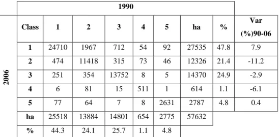
Analysis of table 1 shows that artificial surfaces represented 47.8% of the total area and have increased 7.9% between 1990 and 2006. During this time period, agricultural areas had an important decrease (-11.2%) and lost 1967 ha for artificial areas. Forest and semi-natural areas (-2.9%) and wetlands (-6.1%) also decreased. These classes lost for the artificial areas, respectively, 712 ha and 54 ha.
1990 2006 Class 1 2 3 4 5 ha % Var (%)90-06 1 24710 1967 712 54 92 27535 47.8 7.9 2 474 11418 315 73 46 12326 21.4 -11.2 3 251 354 13752 8 5 14370 24.9 -2.9 4 6 81 15 511 1 614 1.1 -6.1 5 77 64 7 8 2631 2787 4.8 0.4 ha 25518 13884 14801 654 2775 57632 % 44.3 24.1 25.7 1.1 4.8
Table 1 Land use and cover change of CLC level 1 classes (1: Artificial areas; 2: Agricultural areas; 3: Forest and semi natural areas; 4: Wetlands; 5: Water bodies) in the CUB between 1990 and 2006
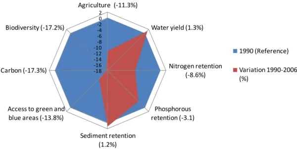
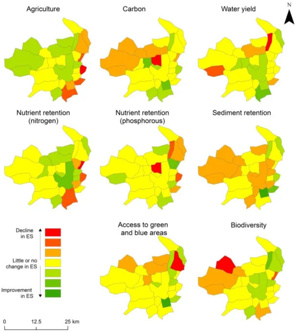
In figure 3 are presented the results for the 8 analyzed ES indicators in the CUB between 1990 and 2006. Only sediment retention had a positive variation in the study area (+1.2%). Water yield is here considered a disservice so its increase (+1.3%) is considered as having a negative effect in flood control. All the other services have evolved negatively during the analyzed time period.
Figure 3 ES indicators variation (%) between 1990 and 2006
In figure 4 is presented the ES variation from 1990 to 2006. Variation of agriculture and biodiversity are represented using the variation in percentage points. All the other ES are represented using variation in percentage. The legend for water yield was inverted so that a increase in the value of this indicator (disservice) is represented using light orange to red color scheme.
-18 -16 -14 -12 -10-8 -6 -4 -20 2 Agriculture (-11.3%) Water yield (1.3%) Nitrogen retention (-8.6%) Phosphorous retention (-3.1) Sediment retention (1.2%) Access to green and
blue areas (-13.8%) Carbon (-17.3%) Biodiversity (-17.2%) 1990 (Reference) Variation 1990-2006 (%)
Figure 4 ES variation between 1990 and 2006
Agriculture is decreasing more importantly on the Eastside of the CUB along the La Garonne river due to urbanization. The carbon storage decreased more importantly on the commune of Bordeaux and on the communes of the NW side of the CUB where it is located the Landes forest. This forest was severely struck by the Martin storm in December 1999 which caused important damages and loss of lives. This effect is also visible in the access to green and blue areas and in biodiversity. Water yield major positive variations, which are considered as negative impacts on flood regulation, is happening mainly in the areas surrounding pre-existing urban areas. Both nitrogen, in the SE, and phosphorous, in the NE, retention are decreasing along the river La Garonne.
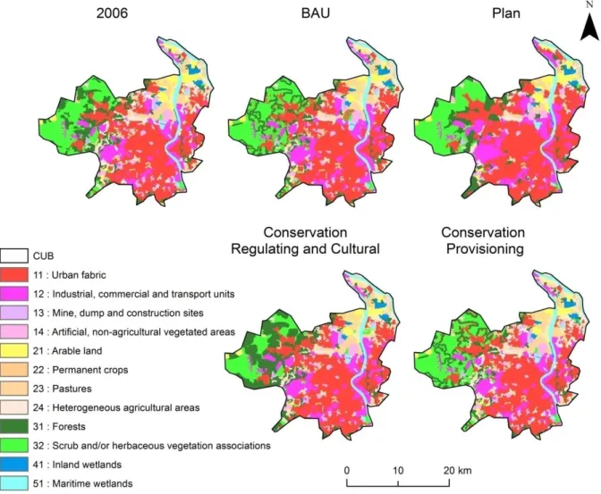
3.2 LULC scenarios for 2030
The LUCC model results are depicted in figure 5. Model validation statistics allocation and quantity disagreement (Pontius and Millones, 2011)presented, respectively,9.4% and 1.57%. These values indicate that
the model is more accurate predicting, for year 2006, quantities than it is in predicting allocation of cells. These values, considering, the number of classes and the temporal proximity between 2000 and 2006, were considered good for the study(Chaudhuri and Clarke, 2014; Estoque et al., 2012).
Figure 6 shows the proportional LULC for 2006 and for each scenario. The "Plan" scenario is the one that accommodates more artificial areas (55.% of total area) being the "Conservation - provisioning" scenario the one more restrictive for this class (47.8%). The "Plan" scenario is the only one that decreases wetlands and water bodies when compared to 2006. Forest and semi-natural areas havevery similar values in all the scenarios. The "Plan" scenario is the one that decreases more the agricultural class (13.5%) and the "Conservation-provisioning" scenario is the only one that increases this class (21.7%) when compared to 2006.
Figure 6Proportional LULC inthe CUBin 2006 and for each scenario
3.3 ES levels for 2030
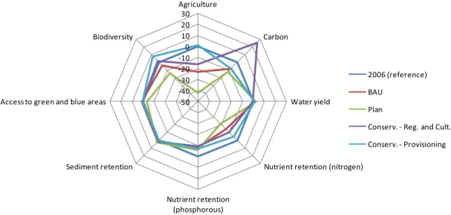
Using the projected LULC for year 2030, ES indicators were calculated using the previously described methods. All biophysical values used in the models were averaged to match the CLC level 2 classification scheme. The "access to green and blue areas" indicator reports the variation (%) of the ha of urban areas in 2006 that are served by the green areas in 2030 of each scenario. In table 2 and figure 7 is shown the joint variation (%)of the ES indicators levels'using CLC 2006 as reference.
ES indicators BAU Plan Conserv. - Reg. and Cult. Conserv. - Provisioning Agriculture -23.2 -41.9 -16.0 1.2 Carbon -7.6 -11.9 25.8 -7.7 Water yield 1.3 2.0 -0.3 0.9 Nitrogen retention -14.4 -21.6 -10.5 -5.1 Phosphorous retention -8.1 -6.1 -9.6 -7.1 Sediment retention 1.5 2.7 1.2 0.1
Access to green and blue areas 0.9 -3.8 0.5 0.3
Biodiversity -3.8 -13.8 1.8 7.9
Table 2 ES indicators variation (%) for the 4 scenarios in 2030 using CLC 2006 as reference (dark red represents a negative variation higher than -10%; light red represents a negative variation between -10 and 0%; light green represents a positive variation between 0 and 10%; dark green represents a positive
variation higher than 10%)
The "BAU" scenario presents slight improvements only in 2 ES: sediment retention (1.5%) and access to green and blue areas (0.9%). The "Plan" scenario only improves sediment retention (2.7%) and degrades very importantly agriculture (-41.9%), carbon storage (-11.9%), nutrient retention (-21.6%) and biodiversity (-13.8%).
47.6 52.6 55.8 51.6 47.8 21.5 16.4 13.5 16.8 21.7 24.9 24.9 25.2 25.6 24.5 1.1 1.1 1.0 1.1 1.1 4.9 4.9 4.5 4.9 4.9 0 20 40 60 80 100 2006 BAU Plan Conservation - Reg. And Cult. Conservation - Provisioning
Artificial areas Agricultural areas
Forest and semi natural areas Wetlands
Both "Conservation scenarios" present a more balances situation. In "Regulation and Cultural Services" scenario carbon storage is strongly improved (25.8%) due to forest preservation. However,there is important degradation in agriculture (-16.9%), nitrogen retention (-10.5%) and phosphorous retention (-9.6%) services. The "Provisioning" scenario is the only that increases agriculture (1.2%) and presents moderate values, both positive and negative, for all the other ES. We note that the nutrient retention, nitrogen and phosphorous, services decline regardless of the scenario used. Although they exhibit different level of degradation, the tradeoff in these services is low and regards only the intensity of the degradation. The same analysis is valid for the sediment retention service which improves in all scenarios.
Figure 7 Joint variation of ES indicators using CLC 2006 as reference
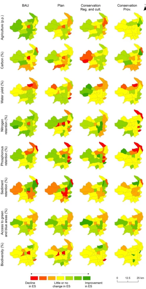
Figure 8 shows the joint variation of ES for all the scenarios using CLC 2006 as reference by administrative area. Orange to red colors represent an increasing decline in the ES between 2006 and 2030, while light green to dark green represent an increasing improvement in the ES.
-50 -40 -30 -20 -10 0 10 20 30 Agriculture Carbon Water yield
Nutrient retention (nitrogen)
Nutrient retention (phosphorous) Sediment retention
Access to green and blue areas Biodiversity
2006 (reference) BAU
Plan
Conserv. - Reg. and Cult. Conserv. - Provisioning
Figure 8 ES joint variation by administrative area for year 2030 according to the scenarios using year 2006 as reference
4. Discussion
This study enabled an integrated assessment of multiple ES under different scenarios of LULC. No or little tradeoffs were found for the nutrient (both nitrogen and phosphorous) and sediment retention services in the landscape of the CUB. This is a consequence of the LUCC scenarios designed with the help of the stakeholders. If these are important ES to be accounted for in the future, the design of scenarios that reflect tradeoffs in these services should be envisaged.
The models used are not necessarily the most sophisticated one's available on the scientific literature and have, as any other models, several limitations(Tallis et al., 2014). However, the advantage of the InVEST tool is to provide a set of open source model's ready to use and available for anyone who wants to do integrated ES assessments in GIS environments. The integrated assessment of ES using spatial data and stakeholder involvement is the most important aspect in the Natural Capital Project approach philosophy which is independent of the models used which can be changed, adapted or replaced by others found more adequate.
Other important aspect we had to deal with was data scarcity.Some datasets had to be calculated using indirect methods, others have disparate collection dates and/or different scales. A considerable effort was made to integrate coherently these datasets. Future versions of the study would benefit from the use of data withimproved resolution and more recent data (e.g. the most recent CLC dates from 2006).
The use of biophysical indicators to study ES is scale-dependent (Gómez-Baggethun and Barton, 2013). Thus, larger scale datasets would enable a more detailed the analysis of these and other urban ES that were not considered due to data technical characteristics and/orunavailability. This was also pointed out by the stakeholders who referred that the scale of analysis did not account for recent green areas that were excluded from the study because they had less than 25 ha, which is the minimum mapping unit of CLC.
This project clearly benefitted from stakeholder participation who were actively involved since the beginning of the project. The selection of relevant ES for the study area, the discussion about the communication(e.g., to report results using administrative areas instead of sub-watersheds) and/or adjustment of specific ES indicators (e.g., access to green areas and biodiversity models) and scenario building were essential for developing an iterative approach that fitted their information needs. Their active participation and willingness to understand the patterns, while recognizing the limitations of the exercise, and how the preliminary results relate to their own activities testified the interest in this type of approach. The scenarios proved to be a powerful discussion tool as they allowed to understand the impact of different planning options on ES.
5. Conclusion
This study aimed an integrated ES assessment enabling an innovative perspective on the functions and uses of the natural environments of the CUB using open data. The results opened a new space for dialogue on a common conceptual and scientific basis for a variety of stakeholders that deal with different subjects. Although the results and the interest shown by stakeholders were promising, the output of scientific model's may not always match the decisions taken by policymakers (Ruiz-Labourdette et al., 2010). Beyond the completion of this study, which will also include an economic analysis to ES, the challenge will be to continue to work on the usefulness of this assessment and the way it can effectively influence decision-making activities contributing to the maintenance of ecosystem functioning.
Acknowledgments
This research is funded by Lyonnaise des eaux. The authors would also like to thank all involved stakeholders and experts that contributed decisively with their opinions and knowledge to the outcome of this project.
References
Bagstad, K J, Semmens, D J, Waage, S, and Winthrop, R, 2013, “A comparative assessment of
decision-support tools for ecosystem services quantification and valuation” Ecosystem
Services5 27–39.
Bagstad, K, Villa, F, Johnson, G, and Voigt, B, 2011, “ARIES—Artificial Intelligence for Ecosystem
Services: A Guide to Models and Data, Version1.0 Beta”.
Boyd, J and Banzhaf, S, 2007, “What are ecosystem services? The need for standardized
environmental accounting units” Ecological Economics63(2-3) 616–626.
Canadell, J, Jackson, R B, Ehleringer, J B, Mooney, H A, Sala, O E, and Schulze, E-D, 1996, “Maximum
rooting depth of vegetation types at the global scale” Oecologia108(4) 583–595.
CGDD, C G au D D and MNHN, M N d’Histoire N, 2010, “Projet de caractérisation des fonctions
écologiques des milieux en France”, Paris,
www.developpement-durable.gouv.fr/Projet-de-caracterisation-des.html.
Chaudhuri, G and Clarke, K C, 2014, “Temporal Accuracy in Urban Growth Forecasting: A Study Using
the SLEUTH Model: Temporal Accuracy in Urban Growth Forecasting: A Study Using the
SLEUTH Model” Transactions in GIS18(2) 302–320.
Chevassus-au-Louis, B, Salles, J-M, and Pujol, J-L, 2009, “Approche économique de la biodiversité et
des services liés aux écosystèmes - Contribution à la décision publique”, Centre d’analyse
stratégique, http://www.ladocumentationfrancaise.fr/rapports-publics/094000203/.
Chisholm, R A, 2010, “Trade-offs between ecosystem services: Water and carbon in a biodiversity
hotspot” Ecological Economics69(10) 1973–1987.
Cruickshank, M M, Tomlinson, R W, and Trew, S, 2000, “Application of CORINE land-cover mapping to
estimate carbon stored in the vegetation of Ireland” Journal of Environmental
Management58(4) 269–287.
CUB, 2012, “55 000 hectares pour la Nature” La Cub Communauté Urbaine de Bordeaux,
http://www.lacub.fr/nature-cadre-de-vie/55-000-hectares-pour-la-nature.
CUB, 2010, “La CUB Open Data” Communauté Urbaine de Bordeaux, http://data.lacub.fr/.
Deletraz, G and Dabos, P, 2001, “Modélisation statistique de la pollution azotée en proximité d’un
axe routier et évaluation des incidences sur l’environnement - Application au site de Biriatou
(A63 – Pyrénées-Atlantiques).”, in (Laboratoire THEMA, Université de Franche-Comté,
INRETS, CERTU, Editions Paradigme), pp 63–93,
http://web.univ-pau.fr/~deletraz/besancon.pdf.
Eastman, R, 2012 Idrisi Selva (Clark Labs).
EEA, 2012, “Corine Land Cover 2006”,
http://www.eea.europa.eu/data-and-maps/data/corine-land-cover-2006-raster-2#tab-metadata.
Estoque, R C, Estoque, R S, and Murayama, Y, 2012, “Prioritizing Areas for Rehabilitation by
Monitoring Change in Barangay-Based Vegetation Cover” ISPRS International Journal of
Geo-Information1(3) 46–68.
EVT, 2012, “Ecosystem Valuation Toolkit”, http://esvaluation.org.
Fagherazzi, S, Marani, M, and Blum, L K, 2004 The Ecogeomorphology of Tidal Marshes (American
Geophysical Union).
Faune d’Aquitaine, 2013, http://www.faune-aquitaine.org/.
Feng, M, Liu, S, Euliss, N H, Young, C, and Mushet, D M, 2011, “Prototyping an online wetland
ecosystem services model using open model sharing standards” Environmental Modelling &
Software26(4) 458–468.
Fisher, B, Turner, R K, and Morling, P, 2009, “Defining and classifying ecosystem services for decision
making” Ecological Economics68(3) 643–653.
FORSEE, 2007, “Un réseau de zones pilotes pour la gestion durable des forêts de l’Arc Atlantique”,
FEDER - INTERREG IIIB Atlantic Area.
Foy, R and Girvan, J, 2004, “An evaluation of nitrogen sources and inputs to tidal waters in Northern
Ireland”,
http://www.ecowin.org/smile/documents/NI%20Nitrogen%20sources%20and%20inputs.pdf.
Gatzweiler, F W, 2006, “Organizing a public ecosystem service economy for sustaining biodiversity”
Ecological Economics59(3) 296–304.
GLAM, 2013, “250-meter MODIS/NDVI Time Series Database”,
http://pekko.geog.umd.edu/usda/test/.
Goldstein, J H, Caldarone, G, Duarte, T K, Ennaanay, D, Hannahs, N, Mendoza, G, Polasky, S, Wolny, S,
and Daily, G C, 2012, “Integrating ecosystem-service tradeoffs into land-use decisions”
Proceedings of the National Academy of Sciences109(19) 7565–7570.
Gómez-Baggethun, E and Barton, D N, 2013, “Classifying and valuing ecosystem services for urban
planning” Ecological Economics86 235–245.
De Groot, R, Brander, L, van der Ploeg, S, Costanza, R, Bernard, F, Braat, L, Christie, M, Crossman, N,
Ghermandi, A, Hein, L, Hussain, S, Kumar, P, McVittie, A, Portela, R, Rodriguez, L C, ten Brink,
P, and van Beukering, P, 2012, “Global estimates of the value of ecosystems and their
services in monetary units” Ecosystem Services1(1) 50–61.
Halpern, B S, Selkoe, K A, Micheli, F, and Kappel, C V, 2007, “Evaluating and ranking the vulnerability
of global marine ecosystems to anthropogenic threats” Conservation biology: the journal of
the Society for Conservation Biology21(5) 1301–1315.
Harley, C D G, Randall Hughes, A, Hultgren, K M, Miner, B G, Sorte, C J B, Thornber, C S, Rodriguez, L
F, Tomanek, L, and Williams, S L, 2006, “The impacts of climate change in coastal marine
systems” Ecology letters9(2) 228–241.
Hédin, L, 1972, “Influence des racines sur la teneur de la matière organique du sol” Fourrages50 83–
96.
Hellweger, F, 1997, “AGREE – DEM surface reconditioning system. Center for Research in Water
Resources”, http://www.ce.utexas.edu/prof/maidment/GISHydro/home.html.
Hijmans, R J, Cameron, S E, Parra, J L, Jones, P G, and Jarvis, A, 2005, “Very high resolution
interpolated climate surfaces for global land areas” International Journal of
Climatology25(15) 1965–1978.
IGN, 2013, “GEOFLA® Communes”, http://professionnels.ign.fr/.
IGN, I N de l’Information G et F, 2006, “BD Carthage v 3.0, descriptif de livraison SHAPEFILE - sphère
eau”,
http://services.sandre.eaufrance.fr/telechargement/geo/BDCarthage/FXX/2012/arcgis/DL_B
DCARTHAGE_3_0_shp.pdf.
INPN, I N du P N, 2013, “INPN - Téléchargements de bases de données”,
http://inpn.mnhn.fr/telechargement/bases-de-donnees.
InVEST, 2013 Integrated Valuation of Environmental Services and Tradeoffs,
http://www.naturalcapitalproject.org/.
Jeanneaux, P, Aznar, O, and Mareschal, S de, 2012, “Une analyse bibliométrique pour éclairer la mise
à l’agenda scientifique des « services environnementaux »” VertigO - la revue électronique en
sciences de l’environnement (Volume 12 numéro 3), http://vertigo.revues.org/12908.
Jeje, Y, 2006, “Export Coefficients for Total Phosphorus, Total Nitrogen and Total Suspended Solids in
the Southern Alberta Region: A Review of Literature”.
Jordan, C, McGuckin, S O, and Smith, R V, 2000, “Increased predicted losses of phosphorus to surface
waters from soils with high Olsen-P concentrations” Soil Use and Management16(1) 27–35.
Kareiva, P, Tallis, H, Ricketts, T H, Daily, G C, and Polasky, S, 2011 Natural Capital: Theory and Practice
of Mapping Ecosystem Services (OUP Oxford, New York).
Kelsey, P and Hall, J, 2010, “Nutrient-export modelling of the Leschenault catchment”, Department of
Water, Western Australia.
Lal, R, 1998, “Soil Erosion Impact on Agronomic Productivity and Environment Quality” Critical
Reviews in Plant Sciences17(4) 319–464.
Lamarque, P, Quétier, F, and Lavorel, S, 2011, “The diversity of the ecosystem services concept and
its implications for their assessment and management” Comptes rendus biologies334(5-6)
441–449.
Langbein, W and Iseri, K, 1995, “Science in Your Watershed - General Introduction and Hydrologic
Definitions”, UNITED STATES GEOLOGICAL SURVEY, Washington, http://water.usgs.gov/wsc/.
Lebourgeois, F and Jabiol, B, 2006, “Enracinements comparés du Chêne sessile, du Chêne pédonculé
Leh, M D K, Matlock, M D, Cummings, E C, and Nalley, L L, 2013, “Quantifying and mapping multiple
ecosystem services change in West Africa” Agriculture, Ecosystems & Environment165 6–18.
Liquete, C, Piroddi, C, Drakou, E G, Gurney, L, Katsanevakis, S, Charef, A, and Egoh, B, 2013, “Current
Status and Future Prospects for the Assessment of Marine and Coastal Ecosystem Services: A
Systematic Review” PLoS ONE8(7) e67737.
Mann, L, Tolbert, V, and Cushman, J, 2002, “Potential environmental effects of corn (Zea mays L.)
stover removal with emphasis on soil organic matter and erosion” Agriculture, Ecosystems &
Environment89(3) 149–166.
Matias, N-G and Johnes, P J, 2011, “Catchment Phosphorous Losses: An Export Coefficient Modelling
Approach with Scenario Analysis for Water Management” Water Resources
Management26(5) 1041–1064.
McKenzie, E, Posner, S, Tillmann, P, Bernhardt, J R, Howard, K, and Rosenthal, A, 2014,
“Understanding the use of ecosystem service knowledge in decision making: lessons from
international experiences of spatial planning” Environment and Planning C: Government and
Policy32(2) 320–340.
Millennium Ecosystem Assessment, 2005 Ecosystems and human well-being: synthesis (Island Press,
Washington, DC).
Mollier, A, 1999 Croissance racinaire du maïs (Zea mays L.) sous déficience en phosphore. Etude
expérimentale et modélisation, Université Paris-Sud, UFR scientifique d’Orsay, INRA
Bordeaux,
https://www.bordeaux-aquitaine.inra.fr/tcem/content/download/2876/29573/version/1/file/These_Mollier_1999.p
df.
Montana DEQ, 2012, “Beaverhead Planning Area Sediment TMDLs and Framework Water Quality
Improvement Plan”, Montana Department of Environmental Quality.
Nahlik, A M, Kentula, M E, Fennessy, M S, and Landers, D H, 2012, “Where is the consensus? A
proposed foundation for moving ecosystem service concepts into practice” Ecological
Economics77 27–35.
NASA/METI, 2012, “ASTER Global DEM data (GDEM V2)”, http://earthexplorer.usgs.gov/.
Nelson, E, Mendoza, G, Regetz, J, Polasky, S, Tallis, H, Cameron, Dr, Chan, K M, Daily, G C, Goldstein,
J, Kareiva, P M, Lonsdorf, E, Naidoo, R, Ricketts, T H, and Shaw, Mr, 2009, “Modeling multiple
ecosystem services, biodiversity conservation, commodity production, and tradeoffs at
landscape scales” Frontiers in Ecology and the Environment7(1) 4–11.
Niemelä, J, Saarela, S-R, Söderman, T, Kopperoinen, L, Yli-Pelkonen, V, Väre, S, and Kotze, D J, 2010,
“Using the ecosystem services approach for better planning and conservation of urban green
spaces: a Finland case study” Biodiversity and Conservation19(11) 3225–3243.
Panagos, P, Van Liedekerke, M, Jones, A, and Montanarella, L, 2012, “European Soil Data Centre:
Response to European policy support and public data requirements” Land Use Policy29(2)
329–338.
Parametrix, 2010, “An introduction to EcoMetrix: Measuring change in ecosystem performance at
the site scale”.
Payraudeau, S, Tournoud, M, Cernesson, F, and Picot, B, 2002, “Modélisation de la charge annuelle
en azote et phosphore par analyse spatiale d’informations topographiques et d’occupation
des sols - Cas d’un petit bassin versant méditerranéen” Revue EAT thématique (Numéro
spécial: Assainissement – Traitement des eaux) 27–35.
Peh, K S-H, Balmford, A, Bradbury, R B, Brown, C, Butchart, S H M, Hughes, F M R, Stattersfield, A,
Thomas, D H L, Walpole, M, Bayliss, J, Gowing, D, Jones, J P G, Lewis, S L, Mulligan, M,
Pandeya, B, Stratford, C, Thompson, J R, Turner, K, Vira, B, Willcock, S, et al., 2013, “TESSA: A
toolkit for rapid assessment of ecosystem services at sites of biodiversity conservation
importance” Ecosystem Services5 51–57.
Pereira, T, Seabra, T, Maciel, H, and Torres, P, 2009, “Portuguese National Inventory Report on
Greenhouse Gases, 1990–2007 submitted under the United Nations Framework Convention
on Climate Change and the Kyoto Protocol” Amadora: Portuguese Environmental Agency.
Peterson, G D, Cumming, G S, and Carpenter, S R, 2003, “Planificación de un Escenario: una
Herramienta para la Conservación en un Mundo Incierto” Conservation Biology17(2) 358–
366.
Petrosillo, I, Zaccarelli, N, and Zurlini, G, 2010, “Multi-scale vulnerability of natural capital in a
panarchy of social–ecological landscapes” Ecological Complexity7(3) 359–367.
Pontailler, J-Y, Hymus, G J, and Drake, B G, 2003, “Estimation of leaf area index using ground-based
remote sensed NDVI measurements: validation and comparison with two indirect
techniques” Canadian Journal of Remote Sensing29(3) 381–387.
Pontius, R G and Millones, M, 2011, “Death to Kappa: birth of quantity disagreement and allocation
disagreement for accuracy assessment” International Journal of Remote Sensing32(15) 4407–
4429.
Raskin, P D, 2005, “Global Scenarios: Background Review for the Millennium Ecosystem Assessment”
Ecosystems8(2) 133–142.
Reckhow, K H, Beaulac, M N, and Simpson, J T, 1980 Modeling Phosphorus Loading and Lake
Response Under Uncertainty: A Manual and Compilation of Export Coefficients (United States
Environmental Protection Agency, Washin).
Renard, K G and Freimund, J R, 1994, “Using monthly precipitation data to estimate the R-factor in
the revised USLE” Journal of Hydrology157(1-4) 287–306.
Rouse, J W, Haas, R H, Schell, J A, and Deering, D W, 1974, “Monitoring vegetation systems in the
Great Plains with ERTS”, in (NASA. Goddard Space Flight Center), pp 309–317.
Ruiz-Labourdette, D, Schmitz, M F, Montes, C, and Pineda, F D, 2010, “Zoning a Protected Area:
Proposal Based on a Multi-thematic Approach and Final Decision” Environmental Modeling &
Assessment15(6) 531–547.
Sleeter, R and Gould, M, 2007, “GIS Software to Remodel Population Data Using Dasymetric Mapping
Methods”, USGS, http://pubs.usgs.gov/tm/tm11c2/tm11c2.pdf.
Swetnam, R D, Fisher, B, Mbilinyi, B P, Munishi, P K T, Willcock, S, Ricketts, T, Mwakalila, S, Balmford,
A, Burgess, N D, Marshall, A R, and Lewis, S L, 2011, “Mapping socio-economic scenarios of
land cover change: A GIS method to enable ecosystem service modelling” Journal of
Environmental Management92(3) 563–574.
Tallis, H and Kareiva, P, 2006, “Shaping global environmental decisions using socio-ecological models”
Trends in Ecology & Evolution21(10) 562–568.
Tallis, H, Rickets, T, Guerry, A, Wood, S, Sharp, R, Nelson, E, Ennaanay, D, Wolny, S, Olwero, E,
Vigerstol, K, Pennington, D, Mendoza, G, Aukema, J, Foster, J, Forrest, J, Cameron, D,
Arkema, K, Lons, E, Kennedy, C, Verutes, G, et al., 2014, “InVEST 3.0.1 User’s Guide:
Integrated Valuation of Environmental Services and Tradeoffs”,
http://ncp-dev.stanford.edu/~dataportal/invest-releases/documentation/current_release/.
Trabucco, A and Zomer, R, 2009, “Global Aridity Index (Global-Aridity) and Global Potential
Evapo-Transpiration (Global-PET) Geospatial Database”, http://www.csi.cgiar.org.
Vihervaara, P, Rönkä, M, and Walls, M, 2010, “Trends in ecosystem service research: early steps and
current drivers” Ambio39(4) 314–324.
Watson, D J, 1947, “Comparative Physiological Studies on the Growth of Field Crops: I. Variation in
Net Assimilation Rate and Leaf Area between Species and Varieties, and within and between
Years” Annals of Botany11(1) 41–76.
Wischmeier, S, 1978, “Predicting rainfall erosion losses: A guide to conservation planning”, U.S.
Department of Agriculture, Washington, DC,
http://topsoil.nserl.purdue.edu/usle/AH_537.pdf.
Wochna, A, Lange, K, and Urbanski, J, 2011, “The influence of land cover change during sixty years on
non point source phosphorus loads to Gulf of Gdansk” JOURNAL OF COASTAL RESEARCH
(Part 2, 64) 1820–1824.
WRI, 2012, “The Corporate Ecosystem Services Review: Guidelines for Identifying Business Risks and
Opportunities Arising from Ecosystem Change”, World Resources Institute, Washington, DC.
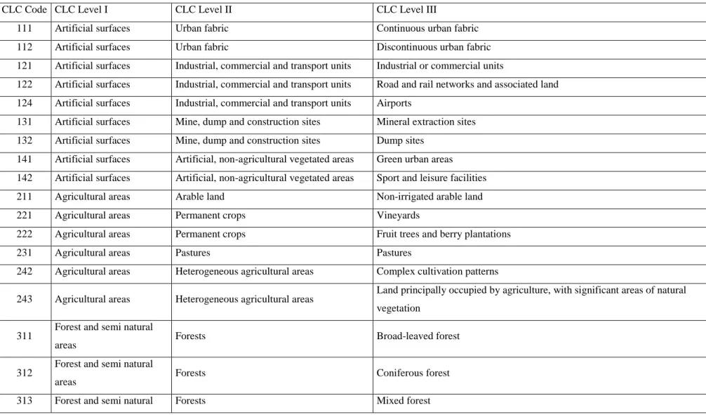
Supplementary Material to: “Ecosystem service monitoring for guiding urban planning in the Urban Community of Bordeaux, France” by Cabral et al. Table A.1. Corine Land Cover classes present in the CUB
CLC Code CLC Level I CLC Level II CLC Level III
111 Artificial surfaces Urban fabric Continuous urban fabric
112 Artificial surfaces Urban fabric Discontinuous urban fabric
121 Artificial surfaces Industrial, commercial and transport units Industrial or commercial units
122 Artificial surfaces Industrial, commercial and transport units Road and rail networks and associated land 124 Artificial surfaces Industrial, commercial and transport units Airports
131 Artificial surfaces Mine, dump and construction sites Mineral extraction sites 132 Artificial surfaces Mine, dump and construction sites Dump sites
141 Artificial surfaces Artificial, non-agricultural vegetated areas Green urban areas 142 Artificial surfaces Artificial, non-agricultural vegetated areas Sport and leisure facilities
211 Agricultural areas Arable land Non-irrigated arable land
221 Agricultural areas Permanent crops Vineyards
222 Agricultural areas Permanent crops Fruit trees and berry plantations
231 Agricultural areas Pastures Pastures
242 Agricultural areas Heterogeneous agricultural areas Complex cultivation patterns
243 Agricultural areas Heterogeneous agricultural areas Land principally occupied by agriculture, with significant areas of natural vegetation
311 Forest and semi natural
areas Forests Broad-leaved forest
312 Forest and semi natural
areas Forests Coniferous forest
areas
321 Forest and semi natural areas
Scrub and/or herbaceous vegetation
associations Natural grasslands
322 Forest and semi natural areas
Scrub and/or herbaceous vegetation
associations Moors and heathland
324 Forest and semi natural areas
Scrub and/or herbaceous vegetation
associations Transitional woodland-shrub
411 Wetlands Inland wetlands Inland marshes
421 Wetlands Maritime wetlands Salt marshes
423 Wetlands Maritime wetlands Intertidal flats
511 Water bodies Inland waters Water courses
512 Water bodies Inland waters Water bodies
Table B.1. Biophysical values used in the InVEST models (ETo: evapotranspiration coefficients; root-depth: root depths in mm; load_n: nutrient load in kg/ha/year; load_p: phosphorous load in kg/ha/year; eff_n: nutrient retention effect in %; eff_p: phosphorous retention in %; usle_c: LULC management factor (value between 0 and 1); usle_p: LULC supporting practice (value between 0 and 1); sedret_eff: sediment retention effect in %, C_soil: amount of carbon stored in soil (in t/ha/year))
CLC
Code ETo root_depth (mm) load_n eff_n load_p eff_p usle_c usle_p sedret_eff C_soil
111 0.094 1 7.75 0.05 1.2 0.05 0.001 0.001 0.1 0 112 0.308 1 7 0.05 1.2 0.05 0.001 0.001 0.05 3.1 121 0.204 1 8 0.05 2.5 0.05 0.001 0.001 0.05 0 122 0.187 1 0.01 0.05 1.2 0.05 0.001 0.001 0.05 0 124 0.292 1 0.01 0.05 2.5 0.05 0.001 0.001 0.05 0.5 131 0.285 1 8.6 0.05 2.5 0.05 0.001 0.001 0.05 0 132 0.195 1 8.6 0.05 2.5 0.05 0.001 0.001 0.05 0 141 0.386 300 1.52 0.05 0.84 0.05 0.001 0.001 0.05 0.9 142 0.43 100 2.5 0.05 1.2 0.05 0.001 0.001 0.05 6.8 211 0.817 900 40 0.25 4.9 0.25 0.5 1 0.25 2.2 221 0.364 2000 5 0.36 1 0.36 0.43 1 0.3 21 222 0.364 2000 10 0.36 1 0.36 0.43 1 0.25 21 231 0.75 100 42.94 0.25 0.84 0.25 0.2 1 0.25 0.9 242 0.75 100 20 0.25 2.32 0.25 0.3 0.8 0.25 1.6 243 0.75 100 15 0.25 0.49 0.25 0.2 0.8 0.25 2 311 0.805 2200 7 0.7 0.23 0.7 0.04 0.45 0.6 38 312 0.84 1200 15 0.8 0.39 0.8 0.04 0.45 0.6 29.9 313 0.822 2200 10 0.8 0.23 0.8 0.04 0.45 0.6 32.8
321 0.355 1000 10 0.4 0.64 0.4 0.01 0.2 0.4 1.5 322 0.549 1000 15 0.65 0.1 0.65 0.1 0.5 0.6 2 324 0.84 1200 10 0.75 0.23 0.75 0.06 0.45 0.6 14.5 411 0.395 2000 0.55 0.8 0.23 0.8 0.003 1 1 1.5 421 0.174 2000 0.55 0.8 0.01 0.8 0.003 1 1 2 423 0.15 2000 0.55 0.8 0.01 0.8 0.003 1 1 0 511 0.012 1 0 0.02 0.5 0.02 0.01 1 0.1 0 512 0.012 1 0 0.02 -6.57 0.02 0.01 1 0.1 0 522 0.012 1 0 0.02 0 0.02 0.01 1 0.1 0