Vol. 34, No. 03, pp. 727 – 738, July – September, 2017 dx.doi.org/10.1590/0104-6632.20170343s20150729
* To whom correspondence should be addressed
A SIMULATION STUDY ABOUT THE IMPACT OF
BIODIESEL USE ON THE ATMOSPHERE OF RIO
DE JANEIRO CITY
R. C. G. Oliveira
1, C. L. Cunha
1, S. M. Corrêa
2*, A. R. Torres
2and E. R. A. Lima
11Chemistry Institute, Rio de Janeiro State University, Rio de Janeiro, RJ, Brazil, 20550-013 2Faculty of Technology, Rio de Janeiro State University, Resende, RJ, Brazil, 27537-000
* Corresponding Author: [email protected]
(Submitted: November 10, 2015; Revised: January 31, 2016; Accepted: April 7, 2016)
Abstract – This study evaluates the impact of biofuels on the air quality of the city of Rio de Janeiro using an air quality model based on the trajectory model OZIPR associated with the SAPRC chemical model. The results show that the increase in biodiesel use reduces ozone levels in the atmosphere by 10.2 %, using Biodiesel with Ethanol and Diesel mixture (BE-Diesel), in 5.28 %, using B20 mixture and only 0.33 % using B10. An increase was observed in NOx emissions of 5.66 and 2.83 % for BE-Diesel mixture and B20, respectively. The low ozone levels are attributed to its consumption by NO. The CO concentration reductions for BE-Diesel, B20 and B10 were 13.11, 6.56 and 4.12 %, respectively. The presence of oxygen atoms within the biodiesel chain leads to a better combustion process, reducing CO emissions.
Keywords: Modeling; Simulation; Biofuels; Air quality.
INTRODUCTION
The Metropolitan Area of Rio de Janeiro (MARJ) is one of the largest urban regions in the world. It covers a total area over 4,690 km2 and represents 11 % of the whole Rio de Janeiro State. Additionally, the MARJ is one of the most industrialized areas in South America and has one of
the largest vehicular fleets in the world, about 2 million
vehicles. The total number of inhabitants is approximately 11 million and the high levels of pollution constitute a critical health problem in the region (INEA, 2011). Besides
this, there are some characteristics which can significantly
increase air quality problems: topography, the presence of a big bay (Guanabara Bay) and several beaches, high temperatures and intense solar radiation, in addition to high population density. Brazilian vehicles use a mixture of anhydrous ethanol added to gasoline since the 1980s (with 20 to 27 % v/v) called gasohol, hydrated ethanol, 7 %
of biodiesel in diesel, and compressed natural gas (CNG),
resulting in a very complex fuel matrix used by the fleet.
The main goal of this study is to evaluate the impact of biofuels on the air quality of the city of Rio de Janeiro and to study scenarios for air quality, due to the increase of biodiesel amount added to diesel (BXX) and ethanol
(BE-Diesel). This study was performed as a first step in
creating a base case with data collected by an automatic monitoring station during three months of the summer season from 2011 to 2012. The base case and scenarios were developed using the trajectory model OZIPR coupled with the chemical mechanism SAPRC.
Volatile Organic Compounds (VOCs) speciation in the atmosphere has been done by several authors in order to obtain a better understanding of the emission sources in urban areas (Blake and Rowland, 1995; Derwent et al., 2000; Na and Kim, 2001; Hsieh and Tsai, 2003; Barletta et al., 2005; Guo et al., 2006; Qin et al., 2007; Langford
of Chemical
et al., 2010). Studies of the VOCs present in the urban atmosphere of Brazilian cities are still scarce and are concentrated in the cities of São Paulo, Rio de Janeiro and Porto Alegre (Grosjean et al., 1998; Vasconcellos et al., 2005; Orlando et al., 2010; Corrêa et al., 2003, 2007, 2010; and Garcia et al., 2013).
In the last decades a considerable reduction in the vehicular emissions was observed due tothe use of new technologies, such as electronic injection, catalysts, and a better fuel quality, following PROCONVE stages (Brazilian Control Program for Air Pollution from Motor Vehicles) where each step or phase requires further reductions in emissions of vehicle pollutants.
Some papers presented previously by Orlando et al. (2010), Garcia et al. (2013), and Souza et al. (2012) used OZIPR to simulate the air quality of great cities, using manual adjustment of the model parameters. In this procedure, variables such as emission rates, deposition
coefficients, and mixing height profile were adjusted by a shooting approach to fit the modeled data. This procedure
demands time, since it did not apply an appropriate parameter estimation procedure and the solution of the problem sometimes was not the best as it could be by using automatic heuristic methods. This paper propose a new approach using particle swarm optimization (PSO) method
in order to estimate parameters and find a minimum value
for the proposed objective function, considering the base case of Rio de Janeiro city.
METHODOLOGY
Site Description
This work used data from SMAC (Environmental Agency of Rio de Janeiro city), collected by an automatic monitoring station located at the State University of Rio de Janeiro (UERJ), from November 2011 to March 2012, from the end of spring to the end ofthe summer season
(22°54′37” S, 43°14’05” W). Data collected included
average hourly values of carbon monoxide (CO), carbon dioxide (CO2), nitrogen oxides (NO and NO2), ozone (O3), sulfur dioxide (SO2), total hydrocarbons (THC), temperature (T), pressure (P), relative humidity (RH), solar
radiation (SR), wind speed (WS) and wind direction (WD).
A sampling campaign for VOCs was carried out beside the automatic monitoring station during January and February, 2012. Two one-hour samples were collected per day: 06:30 h to 07:30 h and 07:30 h to 08:30 h, on the 3rd, 4th, 9th, 16th and 27th days of January 2012, and also February 2nd, 2012. All of these days were without rain, weekdays, and with low cloud cover.
Model Development
The model was built using the trajectory model OZIPR (Ozone Isopleth Package for Research) (Gery and Crouse, 1990; Tonnesen, 2000), which was developed under a
contract with the U.S. Environmental Protection Agency (EPA), as a supporting tool for forecasting scenarios of urban pollution. It is a simple one-dimensional model, known as box or trajectory model, which requires data that include initial concentrations, emissions, and meteorological parameters, with temporal resolution without spatial descriptions of these parameters.It is a dynamic model with concentrated parameters, i.e., the results obtained vary with time but not in space.
This model can be understood as a column of air that covers the studied area up to the mixing layer of the atmosphere, like a box with mobile lid of the height of the mixing layer during the day. The whole box is considered to be homogeneous and moves along the trajectory of the wind, but without horizontal expansion. No topography details are considered in this box model. Emissions from the base of the column and also dry and wet deposition are computed, together with thermal and photochemical reactions (Orlando et al., 2010).
The inputs for the simulation are data from the studied area, including: speciation of the VOCs; initial concentrations of NO, NO2, CO,T, P, RH, and mixing layer height; primary emissions of CO, NOx and THC, location, and date (to calculate the solar irradiation), dry and wet
deposition coefficients, and the chemical mechanism. The
output data are the hourly average concentrations.
The SAPRC (Statewide Air Pollution Research Center) mechanism was initially developed by Carter (1990) and was posteriorly updated by Carter (1994, 1995, 1996), Carter and Atkinson (1996), Carter and Lurmann (1991), and Carter et al. (1997).Itdeals with thermal and photochemical homogeneous reactions, with approximately 140 reactions and 80 species. Species of low importance and with little information regarding the reaction rate and the stoichiometry are not treated explicitly. This can also be used to reduce computational time.
As it is unfeasible to represent the whole chemical mechanism involved, with all explicit species, a methodology that groups them into classes was used. However, some species that have well-established reaction rates and/or are of great importance to the atmospheric chemistry are treated explicitly. The grouping criteria include similarities in structure and reactivity (Carter,
1990). Basically, five groups of alkanes, two groups of
alkenes, four groups of carbonyls, and two groups of aromatics are used.
Emission data
To obtain CO, NOx, and VOCs emission rates, an estimation was performed using the annual emission of CO published by INEA (2009). This report states that theMARJ has an urbanized area of 1,255 km2. To make hourly emission calculations, a year of 313 days (without Sundays and holidays) was considered. For each day, 18 h
of effective vehicle circulation were taken into account, as
Ambient Concentration
The model input data were the initial concentrations of CO, NOx, and VOC speciation. Hourly data of CO, NOx, and O3 concentrations were also needed to compare these data with the values obtained by simulation, in order to adjust the parameters.
Ozone was monitored using an Ecotech PTY Serinus 10, NOx was measured using an Ecotech Serinus 40, NMHC was measured using an Ecotech VOC100 model, CO was measured using an Ecotech Serinus 30 and PM10 and PM2.5 were measured using an Ecotech Spirant BAM.
The VOC sampling methodology was based on TO-15 methodology (U.S.EPA, 1999). It consisted of sampling with 6-L stainless steel canisters, followed by cryogenic pre-concentration of the sample and subsequent analysis by GC-MS using a Varian 450GC 220MS as detailed in Garcia et al. (2013).
For the analysis of formaldehyde and acetaldehyde, the TO-11A methodology (U.S.EPA, 1997) was used. It consists of sampling with SiO2 cartridges coated with C18 and impregnated with 2,4-dinitrophenylhydrazine (DNPH). During sampling, carbonyls are converted into
their hydrazone form. The cartridges were used at a flow rate of 1.0 L min−1 for a period of two hours. The formed
hydrazoneswere eluted from cartridges with acetonitrile and analyzed by HPLC using a C18 column and UV detection at 360 nm (Perkin Elmer series 200), as detailed in Garcia et al. (2013).
Parameters adjustment
The first adjustment of the model parameters was done
to build the basecase. This was performed in two ways:
one manually and another automatic. The first step is to fit
the CO modeled values with experimental values. This is
done first because of its low reactivity and it is essentially
a primary pollutant.
Depending on the discrepancy between the simulated and experimental values, some adjustments are necessary
in the hourly CO emissions to fit these values. The same is
done for NOx and for VOC, as described in detail in the following sections.
In order to use OZIPR one should provide basically three data sets with approximately 84 adjustable variables that would be: emission and deposition rates for CO, NOx
and VOCs, and the height profile of the mixing layer. Manual adjustments are time consuming and difficult to be
correctly performed, due to nonlinearities of the phenomena involved. However, it is important to note that the manual adjustment has been used in all works done previously (Garcia et al., 2013; Souza et al., 2012; Corrêa,2003, 2007, 2010;Orlando, et al., 2010).
In this work, an automatic procedure was designed to make these adjustments in a shorter period of time. The
objective function was defined from the least squares
method weighted by the inverse of the variance following the maximum likelihood principle, according to Equation 2, where the variable Y corresponds to the pollutant
concentration, namely: CO, NOx, O3, σ2 is the variance of the experimental fluctuations of the dependent variable,
Nexp is the number of experiments and Fobj the objective function.
( )
(
_ _)
2 1σ
=−
=
∑
expN
i mod i exp
obj
i i
Y
x
Y
F
In order to automate the comparison between the concentrations calculated by the model (OZIPR) with
those obtained experimentally, a programming effort was
necessary to load the input parameters and run OZIPR for each iteration of the optimization method. It is worth noting that, for each evaluation of the objective functions,
OZIPR needs to be run using the input file containing the
parameters given by the optimization method at that step. Also, after running OZIPR in each step, it is necessary to
get the results from output files of OZIPR and calculate theobjective function from the concentration profiles
predicted.
The optimization algorithm used was the particle swarm optimization (PSO), which is a stochastic optimization
algorithm first proposed by Kennedy and Eberhart (1995).
The idea is to mimic the movement of gregarious animals
in order to perform a method for finding the global
minimum of the objective function automatically. This global minimum in the present study corresponds to the
best set of fitted parameters.
Scenario study for the city of Rio de Janeiro
For creating scenarios, it is first necessary to know the
impact of emissions of each pollutant studied here: CO, NOx and HC. However, as this study did not conduct emission measurements, a study of the current literature was done. Table 1 presents emission rates for Rio de
Janeiro fleet and these data were used to guide the scenarios
presented here. There are several works in the literature in this area, but only some of them could help due to several factors such as: using an engine compatible with the actual
Brazilian fleet in a dynamometer bench in compliance with
Brazilian regulations (ABNT NBR 14489, 2000; ABNT NBR6601, 2005).
Currently in Brazil the average fleet of diesel vehicles
uses B7 in its composition. However, as the studies in 2 1
2
1
1 1
321000
.1000
.
.
.
45
313 18
1255
− −
=
t CO
kg
year
day
kg km h CO
year
t
km
days
h
(1)
the literature compare their results against the emission of standard diesel (B0), this work had to use the same methodology. This work aims to generate scenarios of B10 for light vehicles (SUV), B20 for truck and BE-diesel (diesel with ethanol) for heavy vehicles.
The base case was validated against experimental data and possible variations in emissions were tested. The emissions data for light and heavy vehicles were taken from the work of Anderson (2012).For BE-diesel emissions the work of Shi et al. (2006) was used.
Stratification of the fleet
Emissions considered in this work are the sum from stationary and mobile sources during the three months of
monitoring data. We considered the report by CETESB
(São Paulo State Environmental Agency) regarding vehicle emissions in 2012 (Table 2). The vehicular emissions in São Paulo were used for being the most recent and also
because the fleet of São Paulo and Rio de Janeiro are the
same type.
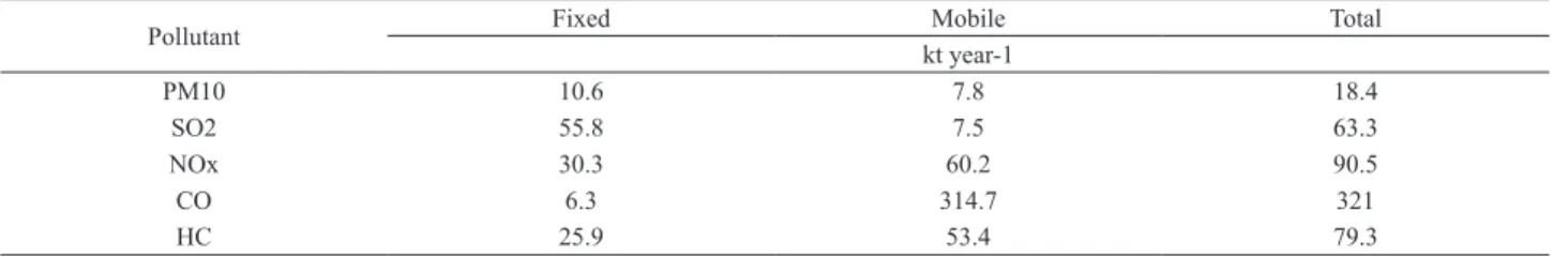
According to Table 1, 98% of CO, 66.5% of NOx and 67.3% of HC are emitted by mobile sources. Of this total, also according to Table 2, 8.36% of CO, 81.54% of NOx and 12.04 % of HC are related to heavy vehicles (buses + trucks). Light diesel vehicles are responsible for 0.40% of CO, 3.67 % of NOx, and 0.57 % of HC.
In this study the emissions profile – that is an input
for the model – was changed according to Table 3. For example, using B20 for heavy vehicles results in an emission reduction of about 4.10 ±6.4 % for CO. So a maximum reduction of 10.5 % and a maximum increase of 2.3 % in the emissions of CO were stipulated. It was performed the same calculation for both HC and NOx for heavy vehicles and light vehicles.
Incremental reactivity scale
To evaluate the VOC incremental reactivity scale, an addition/reduction of 0.2 % of the total VOC for each VOC of interest was performed to calculate ozone changes (Tonnesen, 2000).
Table1. Emission rates by source type in MARJ (INEA, 2009).
Pollutant Fixed Mobile Total
kt year-1
PM10 10.6 7.8 18.4
SO2 55.8 7.5 63.3
NOx 30.3 60.2 90.5
CO 6.3 314.7 321
HC 25.9 53.4 79.3
Table2. Relative contribution of sources ofair pollution(CETESB, 2012).
Vehicles CO (%) HC (%) NOx (%)
light vehicles 57.95 61.10 11.99
light commercial (diesel) 0.40 0.57 3.67
trucks + buses 8.36 12.04 81.54
others 6.80 7.14 1.39
motorcycles 26.49 19.15 1.41
total 100 100 100
Table 3. Summary of emissions data from previous works in the literature.
Source Emissions (%) Blend (%)
CO NOx HC biodiesel ethanol vehicle
U.S.EPA (2002) -11.00 2.00 -21.00 20 - heavy
Shi et al. (2006) 0.00 11.40 -4.20 20 5 heavy
Yanowitz and McCormick (2009) -10.10 2.00 -21.10 20 - heavy
Hoekman et al. (2009) -18.70 -0.60 -21.00 20 - heavy
Hoekman et al. (2009) -10.40 10.80 -17.40 20 - light
Karavalakis et al. (2009) 11.78 13.70 0.00 20 - light
Anderson (2012) -0.70 1.10 -1.60 5 - light
Anderson (2012) 2.70 5.10 4.20 10 - light
Anderson (2012) -4.10 3.50 -5.70 20 - heavy
Kalam et al.a(2011) -21.00 2.00 -17.00 5 - light
Kalam et al.b(2011) -7.30 -1.00 -23.00 5 - light
The average concentration of total VOC measured during the spring of 2012 at UERJ was 1120 ppbC. Therefore, each VOC found in the atmosphere had its concentration increased by 2.24 ppbC (0.2 % of total VOC concentration), while the remaining VOCs were kept unchanged. After this procedure, the fractions were recalculated and loaded into the model. Subsequently, the positive incremental reactivity (IR+) was determined by Equation 3.
[ ]
[ ]
[
]
3 3
0.002.
−
+ =
+
inc base
base
O
O
IR
VOCs
Then, the concentration of each VOC was decreased by 2.24 ppbC. The change in ozone indicates the negative incremental reactivity (IR–).
[ ]
[ ]
[
]
3 3
0.002.
−
− =
−
inc base
base
O
O
IR
VOCs
Although the equations presented for IR+ and IR– are
the same, the results for each IR are different, because
atmospheric chemistry is highly non-linear. The addition/
removal of an individual VOC can lead to different values
for ozone and other secondary pollutants.
It is important to point out that the individual change
for each VOC results in a modification of the speciation of
VOC. Therefore, for each new simulation it is necessary to correct the fraction values of the VOC group.
Finally, the arithmetical average between IR+ and IR- provides the incremental reactivity (IR) for each VOC in MARJ found according to Equation 5.
(
) (
)
2
+ +
−
=
IR
IR
IR
RESULTS AND DISCUSSION
Base case adjustment
The first compound to have its parameters adjusted was
CO for being a primary pollutant with low reactivity. After
performing the best possible fit (closest approach between
the model curve and the experimental curve), changing only the hourly CO emission input, the next step is to
fitthe mixing layer height values. It is worth remembering
that this adjustment occurs around the average values obtained from the emission inventory of INEA. As the
mixing layer height directly influences the concentration
of pollutants, these values were also adjusted to obtain a better approximation. Figure 1 shows the simulated value results compared to the average (experimental) values provided by the automatic monitor between December 21, 2011 and March 21, 2012.
After adjusting the CO input, NOx adjustments were performed. The NOx/CO ratio and VOC/CO ratio
do not remain fixed throughout the day, owing to fleet stratification, which varies throughout the day. In this stage,
an adjustment in the hourly emissions was performed to reproduce the real situation, always keeping the daily average constant. Figure 2 shows the simulated values compared with the average values measured for the period, after the adjustments mentioned.
Once the adjustments were made for CO and NOx,
the base case was then very close to the final stage. The
next step was to adjust the hourly VOC emissions. As the model does not provide data concerning hourly VOC (3)
(4)
(5)
Figure 3. Hourly concentrations of Ozone (ppb) simulated (line) and experimental (symbols) for average days from December 21, 2011 to March 21, 2012 and the respective deviation, using manual adjustment.
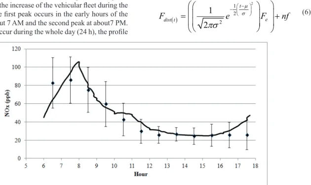
Figure 2. Hourly concentrations of NOx (ppb) simulated (line) and experimental (symbols) for average days from December 21, 2011, to March 21, 2012, and the respective deviation, using manual adjustment.
concentrations, this adjustment should be made using the
ozone profile. A small adjustment in the ozone deposition
rate was also carried out, following the ranges proposed by
Finlayson-Pitts and Pitts (2000) (0.1 to 0.8 cm s−1). The adjusted ozone profile is presented in Figure 3.
The model was loaded with the average initial concentration data (between 6:30 and 9:30 am), hourly emissions of CO, NOx, and VOC, and hourly data for T, RH, mixing layer height, and VOC speciation. These values are shown in Tables 4 and 5.
To attempt fitting the model automatically, a previous
emission behavior study throughout the day was conducted. The emissions of CO, NOx and VOC tend to
follow a profile with two characteristic peaks throughout the day, due to the increase of the vehicular fleet during the rush hours. The first peak occurs in the early hours of the
morning at about 7 AM and the second peak at about7 PM.
As emissions occur during the whole day (24 h), the profile
is not only limited to the morning hours, since emissions are accumulated throughout the day. In other words, there are residual emissions from the previous days (represented by nf), as seen in Figures 4 and 5. For this reason, this work uses a bimodal normal distribution function (two peaks). The purpose here is to reduce the number of input parameters, by working with the distribution parameters, instead of hourly emissions. To reach the purpose it is necessary that the distribution reproduce the experimental
average emissions profile. Equation 6 shows the normal distribution function used where the variables µ, σ, Fe, nf
corresponds to the parameters and t is the time.
( )
2
1 2 2
1
2
µ σ
πσ
− −
=
+
t
e dist t
The emissions data obtained from the manually validated model for each pollutant studied were used to
“train” or adjust the normal distribution function in the
automatic adjustment method, as seen in Figures 4 and 5. As the mixing layer is also important for the adjustment procedure, it is necessary to load into the automatic model
an average height profi le of the mixing layer, as shown in Figure 6. A mixed layer follows a profi le during the day
close to a parabola. Equation 7 gives the curve used to represent the mixing layer.
( )
=
2+ +
F t
at
bt
c
where the variables a, b, c, corresponds the parameters and t is the time.
Therefore, there are a total of 24 input parameters (7 for CO emission, 7 for NOx, 7 for VOC, and 3 for the mixing layer height). Deposition rates were changed, but since there is low sensitivity to changing these values, they were not included in the automatic adjustment.
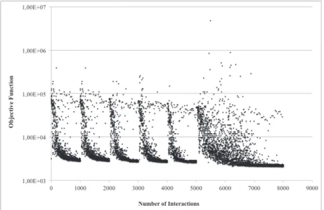
The automatic adjustment response corresponds to a minimum value of the objective function. The total number of iterations is composed of the number of particles and the
number of “fl ights” (steps) used. The number of particles was set to be 40 and the number of fl ights 200, yielding a total of 8000iterations.When the value of the objective
function does not decrease further with increasing iterations, it means that the method found a local minimum
that can be a global minimum or not. When that occurs, it
indicates that a possible solution was obtained, as can be
Table 4. Initial concentrations of VOC, NOx, and CO for the base case.
Compound or group
Initial concentration
CO 0.49 ppm
NOx 0.09 ppm
VOC 1.12 ppmC
Table 5. Values for temperature, relative humidity, mixing layer height for the base case.
Hour T (ºC) RH (%) Mixing
height (m)
06:30 25.37 77.76 200
07:30 26.72 72.10 250
08:30 28.16 65.74 300
09:30 29.33 60.24 650
10:30 30.44 56.00 1000
11:30 31.53 51.78 1450
12:30 32.13 50.12 1600
13:30 32.33 49.76 1700
14:30 32.28 50.05 1750
15:30 31.77 52.07 1050
16:30 31.07 53.86 800
17:30 30.10 56.27 400
Figure 4. CO profi lealong a typical day for Rio de Janeiro city. Figure 5. NOx profi le along a typical day of Rio de Janeiro city.
seen in Figure 7. In order to ensure that the global minimum has been found, the algorithm must be run several times.
It can be observed in Figure 7 that, in the fi rst iterations,
the stochastic optimization method PSO searches the entire
region of study. Subsequently, the particles “communicate”
with each other and the swarm is guided by the best answers
obtained and fi nally reaches a minimum of the objective
function. To start a new iteration, the best parameters that led to the lowest objective function are included in the next iteration of the algorithm, thus getting faster convergence to a minimum objective function.
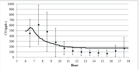
Figure 8 presents the results obtained for the concentration of CO using the automatic procedure. The adjustment performed here has some deviations from the experimental values, even considering the errors bars. The manual adjustments presented in Figure 1 showed a better adjustment. However, considering the time-consuming
procedure for the manual adjustment, the fast automatic adjustment can be considered acceptable.
For the concentration of O3 (Figure 9), the profi le
automatically adjusted during the day did not result in a very good answer. The model overestimates the concentration of O3 at the end of the day. As a secondary pollutant, O3 is formed by photochemical reactions involving NOx and VOC.
The attempt of using an automatic procedure for setting the parameters proved to be useful as it serves as a method for an initial adjustment. The automatic adjustment method becomes an excellent starting point. From its result, it is
straightforward to do the fi ne adjustment manually, by
using heuristic rules that are not so easy to automate, in
order to fi nd the best answer. Therefore, the use of this automatic fi rst step for adjusting the parameters means a great decrease in the time necessary tofi nd the best answer,
Figure 6. Mixing height profi le simulated and experimental for the day 01/16/2012 for manual adjustment.
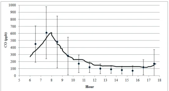
Figure 8. Hourly concentrations of CO (ppb) simulated using the automatic adjustment and experimental data for average days between December 21, 2011, to March 21, 2012, and the respective deviation bars for each time of day.
Figure 9. Hourly concentrations of O3 (ppb) simulated and experimental for average days between December 21, 2011, to March 21, 2012, and their deviation bars for each time of day for the automatic adjustment.
since the purely manual adjustment is very time consuming. To improve the results obtained from the automatic procedure it is necessary to better understand the atmospheric phenomena involved for each pollutant previously studied. This wayit is possible to change the objective function to prioritize more relevant points at the expense of others not so important (by using weights). Thus, it would be possible to propose an objective function that gives priority to the most important measurements,
making the search more efficient. This is a good challenge
for future works in the area.
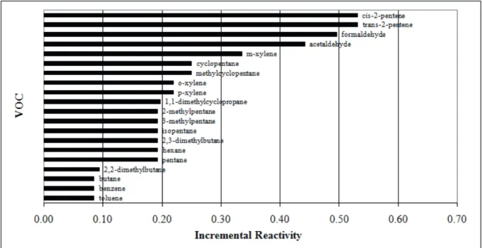
To quantify the VOCs incremental reactivity, a study was performed with the 20 major VOC ozone precursors in
the city of Rio de Janeiro during the summer base case. We note that the alkenes have more influence on the results, as
these molecules are very reactive, as detailed in Figure 10.
Taking as example the case of formaldehyde, Figure 10 indicates that increasing 1.0 µg·m-3 the concentration of formaldehyde, while keeping unchanged all the other VOC leads to an increase in ozone of 0.5 µg·m-3. Thus, the incremental reactivity scale may be a useful tool for decision makers in order to minimize the emission of more reactive VOC. As possible applications of this study we can mention givingsubsidiesto petrochemical companies in the formulationof fuels andfor environmental institutes on the regulation to reduce emissions of certain molecules by respective sources.
Besides the results for the scenarios studied, the model also allows performing multiple simulations of maximum
ozone produced from different concentrations of VOCs
Figure 10. Incremental Reactivity scale for the main VOCs at MARJ.
Figure 11. Ozone isopleths (ppb) for various concentrations of VOC and NOx, for the ase case.
a function of NOx and VOCs. The region where the two straight lines intersect corresponds to the base case for the city of Rio de Janeiro. According to Figure 11, one can see that there is a tendency to decrease the concentration of O3 as the concentration of NOx increases. On the other hand, the concentration of O3 increases as the VOCs concentrations increase.
For scenarios with the B10, B20 and BE-diesel there are a decrease in ozone concentration. The greater
concentration of oxygenates in biodiesel causes a higher combustion temperature and consequently an increase in NOx emissions to the atmosphere. These results are presented in Table 6.
Table 6. Values for pollutants with additional use of biodiesel and BE-Diesel.
Pollutants Base case B10 B20 BE – Diesel Hour
ppb
CO max 610 580 570 530 8:00
NOx max 106 106 109 112 8:00
O3 max 30.3 30.2 28.7 27.2 14:00
BE-Diesel showed up as the best option among mixtures of fuels covered in this study. Possibly, this is due to the inclusion of ethanol as an additive, having improved fuel combustion in the engine. However, it is noteworthy that there is a small increase in the concentration of NOx in the atmosphere, which is harmful to human beings.
Changesin the concentration values of the pollutants listed in Table 6are small because much of the emissions
are due to fixed sources or mobile sources not included in
the study, leaving only a small portion for mobile sources covering heavy or light vehicles (trucks) that use diesel as fuel.
A study where the concentration of heavy vehicles is higher, as in the case of highways, can lead to results with
greater differences in the peak values of the pollutants.
CONCLUSIONS
This work presents a contribution o the understanding of legislated concentrations of pollutants in the city of Rio de Janeiro, as well as the contribution of these compounds to the tropospheric O3 concentration. The base case was developed and reproduced the experimental data for
“manual” parameter setting, based on heuristic rules.
An automatic procedure for parameter adjustment has been proposed as an attempt to represent the average
emission profile for each pollutant in the city of Rio de Janeiro, in order to express this profile through a
well-known mathematical function. This study demonstrated thatthe automatic adjustment could substantially decrease
the adjustment effort, but did not lead to better answers in
this situation. Thus, it can be used as an initial step before
the “fine” manual parameters adjustment.
The scenarios studied here tested the impact of increasing the fraction of biodiesel or ethanol indiesel. The results obtained for CO and O3 showed a small decrease in the concentration of pollutants in the city of Rio de Janeiro in this situation. Nevertheless, the presence of oxygen in biodiesel and ethanol causes the increase in the emission and concentration of NOx, and leads to the increased consumption of O3 in the troposphere. Moreover, there is a better burning of the fuel, generating a lower concentration of CO in the atmosphere. However, there was an increasein the concentration of NOx in these scenarios.
It could also be observed in the study of isopleth curves that the urban atmosphere of the city of Rio de Janeiro is controlled by NOx.
The results of this study confirm the environmental
issues related to economic development, especially in large urban centers. Air pollution results from the lack of collective thinking in regarding to air quality. The increase
in the vehicular fleet in metropolitan regions justifies more academic research in this field. Thus, knowledge about
the contribution of emissions generated by the operation of these vehicles and the search for cleaner technologies should be deeply encouraged. Furthermore, strict regulations and oversight by the government is necessary
to assure the specifications will be met.
ACKNOWLEDGMENTS
The authors are thankful for data supported by
CETESB, INEA, SMAC and for the financial support by
CAPES, CNPq and FAPERJ.
REFERENCES
ABNT NBR 6601. Determination of hydrocarbon, carbon monoxide, nitrogen oxide, carbon dioxide and particulate material on exhaust gas. Rio de Janeiro, Brazil (2005).
ABNT NBR 14489. Diesel engine - Analysis and evaluation of gases and particulate matter emitted by the diesel engine - 13 mode cycle. Rio de Janeiro, Brazil (2000).
Anderson, L.G., Effects of biodiesel fuels use on vehicle
emissions. Journal of Sustainable Energy Environment, 3, 35 (2012).
Barletta, B., Meinardi, S., Rowland, F.S., Chan, C-Yu, Wang, X.,
Zou, S., Chan, L.Y., Blake, D.R., Volatile organic compounds in 43 Chinese cities.Atmospheric Environment, 39, 5979 (2005).
Blake, D.R., Rowland, F.S., Urban leakage of liquefied petroleum
gas and its impact on Mexico City air quality.Science,269, 953 (1995).
Carter, W.P.L., A detailed mechanism for the gas-phases
atmospheric reactions of organic compounds. Atmospheric Environment, 24, 481 (1990).
Carter, W.P.L., Development of ozone reactivity scales for volatile organic compounds. Journal of the Air &Waste Management
Association, 44, 881 (1994).
Carter, W.P.L., Computer modeling of environmental chamber
studies of maximum incremental reactivities of volatile organic compounds. Atmospheric Environment, 29, 2513 (1995).
Carter, W.P.L., Condensed atmospheric photooxidation
Carter, W.P.L., Atkinson, R., Development and evaluation of a
detailed mechanismfor the atmospheric reactions of isoprene and NOx. International Journal of Chemical Kinetics, 28, 497 (1996).
Carter, W.P.L., Luo, D., Malkina, I.L., Environmental chamber
studies for development of an update photochemical mechanism for VOC reactivity assessment. Final Report to the California Air Resources Board, Contract 92- 345 (1997).
Carter, W.P.L.,Lurmann, F.W., Evaluation of a detailed
gas-phase atmospheric reaction mechanism using environmental chamber data. Atmospheric Environment, 25, 2771 (1991). CETESB.
<http://www.cetesb.sp.gov.br/ar/qualidade-do-ar/31-publicacoes-e-relatorios>. Acessed in February 2, 2013. CETESB. Qualidade do ar: poluentes.<http://www.cetesb.
sp.gov.br/ar/ /emissao-veicular/48-relatorios-e-publicacoes>. Accessed in January 1, 2013.
CETESB. Air quality report for the São Paulo state, ISSN0103-4103 (2012).
CETESB. Air quality report for the São Paulo state,ISSN0103-4103 (2011).
Corrêa, S.M., Martins, E.M., Arbilla, G., Formaldehyde and
acetaldehyde in a high traffic street of Rio de Janeiro.
Atmospheric Environment, 37, 23 (2003).
Corrêa, S.M., Arbilla, G., A two-year of aromatic hydrocarbons monitoring at the downtown area of the city of Rio de Janeiro. Journal of the Brazilian Chemical Society, 18, 539 (2007).
Corrêa, S.M., Arbilla, G., Martins, E.M., Quitério, S.L., Guimarães, C.S., Gatti, L.V., Five-years of formaldehyde and acetaldehyde monitoring in the Rio de Janeiro downtown area - Brazil. Atmospheric Environment, 44, 2302 (2010). Derwent, R.G., Davies, T.J., Delaney, M., Dollard, G.J., Field,
R.A., Dumitrean, P., Nason, P.D., Jones, B.M.R., Pepler, S.A., Analysis and interpretation of the continuous hourly monitoring data for 26 C2-C8 hydrocarbons at 12 United Kingdom sites during 1996. Atmospheric Environment, 34, 297 (2000).
Finlayson-Pitts, B.J.,Pitts, J.N., Chemistry of the upper and lower atmosphere.San Diego: Academic Press (2000).
Garcia, L.F.A., Corrêa, S.M., Penteado, R., Daemme, L.C., Gatti, L.V., Alvim, D.S., Measurements of emissions from motorcycles and modeling its impact on air quality. Journal of the Brazilian Chemical Society, 24, 375 (2013).
Gery, M.W., Crouse, R.R.,
User’s guide for executing OZIPR. U.S. Environmental
Protection Agency (1990).
Grosjean, E., Rasmussen, R.A., Grosjean, D., Ambient levels of gas phase pollutants in Porto Alegre, Brazil. Atmospheric Environment, 32, 3371 (1998).
Guo, H., Wang, T., Blake, D. R., Simpson, I. J., Kwok, Y. H., Li, Y.
S., Regional and local contributions to ambient nonmethane volatile organic compounds at a polluted rural/ coastal site in Pearl River Delta, China. Atmospheric Environment, 40, 2345-2359 (2006).
Hoekman, S.K., Gertler, A., Broch, A., Robbins, C., Investigation of biodistillates as potential blendstocks for transportation fuels CRC project No. AVFL-17, Coordinating Research Council, Inc. (2009).
Hsieh, C.C., Tsai, J.H., VOC concentration characteristics in southern Taiwan. Chemosphere, 50, 545 (2003).
INEA, 2009.Annual air quality report for the Rio de Janeiro state. http://www.inea.rj.gov.br/downloads/relatorios/qualidade_ ar_2009.pdf. Accessed in January 4, 2013.
INEA, 2011. Annual air quality report for the Rio de Janeiro state. http://www.inea.antigo.rj.gov.br/fma/qualidade-ar.asp. Accessed in July 13, 2015.
Kalam, M.A., Masjuki, H.H., Jayed, M.H., Liaquat, A.M., Emission and performance characteristics of an indirect ignition diesel engine fuelled with waste cooking oil. Energy, 36, 397 (2011).
Karavalakis, G., Alvanou, F., Stornas, S., Bakeas, E., Regulated and unregulated emissions of a light duty vehicle operated on diesel/palm-based methyl ester blends over NEDC and a non-legislated driving cycle. Fuel, 88, 1078 (2009).
Kennedy, J., Eberhart, R., Particle swarm optimization. In: Proceedings of the IEEE international conference on neural networks, Perth, Australia, v. 4, 1942 (1995).
Langford, B., Nemitz, E., House, E., Phillips, G.J., Famulari, D., Davison, B., Hopkins, J.R., Lewis, A.C., Hewitt, C.N., Fluxes and concentrations of volatile organic compounds above central London, UK. Atmospheric Chemistry and Physics, 10, 627 (2010).
Na, K.,Kim, Y.P., Seasonal characteristics of ambient volatile organic compounds in Seoul. Atmospheric Environment, 35, 2603 (2001).
Orlando, J.P., Alvim, D.S., Yamazaki, A., Corrêa, S.M., Gatti, L.V., Ozone precursors for the São Paulo metropolitan area. Science of the Total Environment, 408, 1612 (2010).
Qin, Y., Walk, T., Gary, R., Yao, X., Elles, S.,C2-C10 nonmethane
hydrocarbons measured in Dallas, USA—Seasonal trends and diurnal characteristics. Atmospheric Environment, 41, 6018 (2007).
Shi, X., Xiaobing, P., Yujing, M., Hong, H., Shijin, S., Jianxin,
W., Hu, C., Rulong, L., Emission reduction potential of using
ethanol–biodiesel–diesel fuel blend on a heavy-duty diesel engine. Atmospheric Environment, 40, 2567 (2006).
Souza, C.V., Corrêa, S.M., Sodré, E.D., Teixeira, J.R., Volatile
organic compound emissions from a landfill, plume dispersion
and the tropospheric ozone modeling. Journal of the Brazilian Chemical Society, 23, 496 (2012).
Tonnesen, G.S., User’s guide for executing OZIPR version 2.0.
North Caroline: U.S.EPA (2000).
U.S. EPA. Compendium method TO-11. Determination of formaldehyde in ambient air using adsorbent cartridge followed by high performance liquid chromatograph. EPA/625/R-96/010b (1997).
U.S.EPA. Compendium method TO-15. Determination of volatile organic compounds (VOC) in air collected in specially-prepared canisters and analyzed by gas chromatography/mass spectrometry. EPA/625/R-96/010b (1999).
Vasconcellos, P.C., Carvalho, L.R.F., Pool, C.S., Volatile organic compounds inside urban tunnels of São Paulo city, Brazil. Journal of the Brazilian Chemical Society, 16, 1210 (2005).
Yanowitz, J., McCormick, R.L., Effect of biodiesel blends